R E S E A R C H
Open Access
Delta shock wave with Dirac delta
function in multiple components for the
system of generalized Chaplygin gas
dynamics
Yicheng Pang
**Correspondence: [email protected] School of Mathematics and Statistics, Guizhou University of Finance and Economics, Guiyang, 550025, China
Abstract
We study the Riemann problem for the compressible Euler equations with the generalized Chaplygin gas. Based on the analysis on the physically relevant region, we obtain five kinds of exact solutions. It is shown that a delta shock wave with Dirac delta function in both density and internal energy develops in the exact solutions. The formation mechanism, generalized Rankine-Hugoniot relation and entropy condition are clarified for this type of delta shock wave. The numerical results are also presented to confirm this type of delta shock wave.
Keywords: delta shock wave; generalized Chaplygin gas; Euler equations; Riemann problem
1 Introduction
The compressible Euler equations are governed by
⎧ ⎪ ⎨ ⎪ ⎩
ρt+ (ρu)x= ,
(ρu)t+ (ρu+p(ρ,s))x= ,
(ρu/ +ρe)
t+ ((ρu/ +ρe+p(ρ,s))u)x= ,
(.)
where the variablesρ, u,s,p,edenote density, velocity, specific entropy, pressure, and specific energy. Bothpandeare given functions ofρands, satisfying the thermodynamical constraint
Tds= de+pd
ρ, (.)
whereT =T(ρ,s) is the temperature. Considerable progress has been made on the Rie-mann problems or other closely related problems for system (.) with the polytropic gas; see [–] and the references therein. Here, we concern ourselves with the equation of state
p(ρ,s) = –Aρ–α, (.)
which is called the generalized Chaplygin gas, where <α≤,A> are constants. A sub-stantial difference between the polytropic gas and the generalized Chaplygin gas is that the latter has a negative pressure with a positive sound speed. The generalized Chaplygin gas is used as a unified description for the recent accelerated expansion of the universe and the evolution of the perturbations of energy density. It has also emerged as a uni-fication of dark energy and dark matter. Equation (.) withα= is called a Chaplygin gas, which was introduced by Chaplygin [] and Tsien [] as a mathematical approxi-mation for calculating the lifting force on a wing of an airplane in aerodynamics. The reader is referred to [–] for more physical background on the generalized Chaplygin gas.
Recently, the (generalized) Chaplygin gas has attracted intensive attention. Brenier [] considered the Riemann problem for the isentropic Euler equations
ρt+ (ρu)x= ,
(ρu)t+ (ρu+p(ρ,s))x= ,
(.)
with the Chaplygin gas, where the solutions with concentration were obtained when the initial data belong to a certain domain in the phase plane. Guoet al.[] removed this constraint, and they obtained the delta shock wave solutions. Roughly speaking, the delta shock solution is a solution such that at least one of the state variables has a Dirac delta function []. Physically, the delta shock waves are interpreted as the process of formation of the galaxies in the universe, or the process of concentration of particles. For the theory of delta shock wave and its related topics, the reader is referred to [] for a more detailed review. Wang [] constructed the Riemann solutions to system (.) for the generalized Chaplygin gas, while the formation of a delta shock wave and vacuum state for system (.) as pressure vanishes was analyzed by Shenget al.[]. In addition, Sun [] dealt with the Riemann problem of system (.) with the Coulomb-like friction term for the generalized Chaplygin gas, and the delta shock wave solutions were constructed. However, in contrast to the extensive investigations on the isentropic Euler equations (.) with the (general-ized) Chaplygin gas, little literature contributed to the compressible Euler equations (.) with the (generalized) Chaplygin gas.
consider the compressible Euler equations of the form
⎧ ⎪ ⎨ ⎪ ⎩
ρt+ (ρu)x= ,
(ρu)t+ (ρu+p(ρ,s))x= ,
(ρu/ +H)
t+ ((ρu/ +H+p(ρ,s))u)x= ,
(.)
where the state variableH≥ is the internal energy.
We study the Riemann problem for (.) and (.) with the initial data
(ρ,u,H)(,x) =
(ρ–,u–,H–), x< ,
(ρ+,u+,H+), x> ,
(.)
whereρi> ,ui,Hi> ,i= –, +, are different constants. In a recent paper, the case where α= was solved. It was found that a delta shock wave with Dirac delta function in both density and internal energy appeared in the solutions. Meanwhile, the formation mecha-nism of this kind of delta shock wave results from the overlapping of the linearly degener-ate characteristic lines. In this article, we pay attention to the case where <α< .
In the generalized Chaplygin gas <α< , with the thermodynamical constraint (.), we first conduct the physically relevant region for system (.) and (.). Then, based on the projections of the classical wave curves onto the (ρ,u)-plane, the Riemann problem is di-vided into two cases. In the caseu––
√
Aρ––(+α)/<u++ √
Aρ+–(+α)/, by the analysis on the
physically relevant region and the method of characteristic analysis, we obtain four kinds of exact solutions, which are the combination of a centered rarefaction wave, a shock wave, and a contact discontinuity. However, for the caseu––
√
Aρ––(+α)/≥u++ √
Aρ+–(+α)/,
the Riemann problem cannot be solvable by a combination of these classical waves. In this case, we justify rigorously the phenomenon of the delta shock wave with a Dirac delta function in both density and internal energy. We then propose both a generalized Rankine-Hugoniot relation and an entropy condition for this type of delta shock wave. Using these relations, the delta shock wave solution is obtained in this case, in which both density and internal energy contain the Dirac delta function simultaneously. Meanwhile, the expres-sions for the location, speed, and weights of this type of delta shock wave are explicitly provided. Finally, we present the numerical results, performed by the Nessyahu-Tadmor scheme [], to confirm this type of solution.
In our study, it is shown that the delta shock wave with Dirac delta function in both den-sity and internal energy develops in the compressible Euler equations with the generalized Chaplygin gas. To the best of our knowledge, this type of delta shock wave has not been found in the previous studies on the generalized Chaplygin gas. Besides, the formation mechanism of this kind of delta shock wave in the generalized Chaplygin gas results from the overlapping of the linearly degenerate and genuinely nonlinear characteristic lines, which is substantially different from the case of the Chaplygin gas. Moreover, this type of delta shock wave has also been illustrated numerically.
and an entropy condition of this type of delta shock wave. We also give the numerical results to confirm this type of delta shock wave. The conclusion is given in Section .
2 Solutions involving classical waves 2.1 Classical waves
We derive the physically relevant region for the system (.) and (.). One shows from (.) thatTds= d(e–αA+ρ–(α+)). Thus, there exists a functionf(s) such that
T=f(s), e= A
α+ ρ
–(α+)+f(s).
The positivity ofeshows that the power functiong(X) =αA+X(α+)+f(s),X∈(, +∞) takes
positive values. This implies thatf(s)≥, namely,e–αA+ρ–(α+)≥. Therefore, the
phys-ically relevant region is
ℵ=
(ρ,u,H)ρ> ,H≥ A
α+ ρ
–α
,u∈R . (.)
The system (.) and (.) has three eigenvalues
λ=u–
Aαρ–(α+), λ
=u, λ=u+
Aαρ–(α+), (.)
with the corresponding right eigenvectors
r=
ρ, –Aαρ–(α+),H+pT, r
= (, , )T, r=
ρ,Aαρ–(α+),H+pT,
satisfying∇λ·r=α–
Aαρ–(α+)< ,∇λ
·r=–α
Aαρ–(α+)> ,∇λ
·r= . Hence,
the first and third characteristic fields are genuinely nonlinear, while the second one is linearly degenerate.
Both (.) and (.) remain invariant under the transformation (t,x)→(αt,αx),α> , so we need to seek a self-similar solution (ρ,u,H)(ξ) (ξ =x/t). Therefore, the Riemann problem for (.), (.), and (.) can be reduced to the following boundary value problem at infinity:
⎧ ⎪ ⎪ ⎪ ⎨ ⎪ ⎪ ⎪ ⎩
–ξρξ+ (ρu)ξ = ,
–ξ(ρu)ξ+ (ρu+p)ξ = ,
–ξ(ρu/ +H)
ξ+ ((ρu/ +H+p)u)ξ = ,
(ρ,u,H)(±∞) = (ρ±,u±,H±).
(.)
For smooth solutions, we can rewrite (.) in the matrix form
⎛ ⎜ ⎝
u–ξ ρ
Aαρ–(+α) (u–ξ)
H–Aρ–α u–ξ
⎞ ⎟ ⎠
⎛ ⎜ ⎝ ρ
u H
⎞ ⎟ ⎠
ξ
= . (.)
Thus, besides the constant solution (ρ,u,H) = Const., it provides either a backward cen-tered rarefaction wave
←–
R: ξ=u–Aαρ–(α+), du
dρ = – √
Aαρ–(α+)/, dH
dρ = (H+p)ρ
or a forward centered rarefaction wave
–
→
R: ξ=u+Aαρ–(α+), du
dρ = √
Aαρ–(α+)/, dH
dρ = (H+p)ρ
–. (.)
Given a left state (ρ–,u–,H–), we integrate (.) and take the requirementλ(ρ–,u–) < λ(ρ,u) to obtain the backward centered rarefaction wave curve
←–
R(ρ–,u–,H–): ⎧ ⎪ ⎨ ⎪ ⎩
ξ=u–√Aαρ–(α+)/, u=
√
Aα
+α ρ
–(α+)/+u ––
√
Aα
+α ρ
–(α+)/
– ,
H= A +αρ
–α+ ρ ρ–(H––
A +αρ
–α
– ),
ρ<ρ–, (.)
which is the set of the states that can be connected to the left state (ρ–,u–,H–) on the
right by a backward centered rarefaction wave. Similarly, for a given right state (ρ+,u+,H+),
integrating (.) and using the requirement λ(ρ+,u+) >λ(ρ,u), we derive the forward
centered rarefaction wave curve
–
→
R(ρ+,u+,H+): ⎧ ⎪ ⎨ ⎪ ⎩
ξ=u+√Aαρ–(α+)/,
u= – √
Aα
+α ρ
–(α+)/+u ++
√
Aα
+α ρ
–(α+)/
+ ,
H=+Aαρ–α+ρρ
+(H+–
A +αρ
–α
+ ),
ρ<ρ+, (.)
which consists of the states that can be joined with the right state (ρ+,u+,H+) on the left
by a forward centered rarefaction wave.
For a bounded discontinuous solution with a discontinuityξ=ω, the Rankin-Hugoniot condition for (.) and (.) is
⎧ ⎪ ⎨ ⎪ ⎩
–ω[ρ] + [ρu] = , –ω[ρu] + [ρu+p] = ,
–ω[ρu/ +H] + [(ρu/ +H+p)u] = ,
(.)
whereωis the velocity of the discontinuity, and [G] =G+–G–, withG–andG+the values
of the functionGon the left and right-hand sides of the discontinuity, is the jump ofG across the discontinuity. We obtain by calculating (.) either a backward shock wave
←– S: ⎧ ⎪ ⎨ ⎪ ⎩
ω=u––
ρ+[p]
ρ–[ρ]=u+–
ρ–[p]
ρ+[ρ],
[u] = –
[p]
ρ+ρ–[ρ][ρ], [H] =ρ –
– (H–+(p++p–))[ρ],
(.)
a contact discontinuity
J: ω=u–=u+, [ρ] = , [u] = , [H]= , (.)
or a forward shock wave
– → S: ⎧ ⎪ ⎨ ⎪ ⎩
ω=u–+
ρ+[p]
ρ–[ρ] =u++
ρ–[p]
ρ+[ρ],
[u] =
[p]
ρ+ρ–[ρ](ρ+–ρ–), [H] =ρ
–
+ (H++(p++p+))[ρ].
(.)
For a given left state (ρ–,u–,H–), by (.) and the entropy condition of the shock wave
a backward shock wave curve can be expressed as
←–
S(ρ–,u–,H–): ⎧ ⎪ ⎪ ⎪ ⎨ ⎪ ⎪ ⎪ ⎩
ω=u––
ρ[p]
ρ–[ρ]=u–
ρ–[p]
ρ[ρ],
u=u––
[p]
ρρ–[ρ](ρ–ρ–),
H= –(p+p–) +ρρ–(H–+
(p+p–)),
ρ>ρ–, (.)
which is the set of the states that can be connected to the left state (ρ–,u–,H–) on the right
by a backward shock wave. Using (.), it is easy to obtain a contact discontinuity curve
J(ρ–,u–,H–): ω=u=u–, ρ=ρ–, u=u–, H=H–, (.)
which is the set of the states that can be joined with the left state (ρ–,u–,H–) by a
con-tact discontinuity. Besides, for a given right state (ρ+,u+,H+), using (.) and the entropy
condition of a shock wave,
λ(ρ+,u+) <ω<λ(ρ,u), ω>λ(ρ,u), (.)
we obtain a forward shock wave curve
–
→
S(ρ+,u+,H+): ⎧ ⎪ ⎪ ⎪ ⎨ ⎪ ⎪ ⎪ ⎩
ω=u++
ρ[p]
ρ+[ρ]=u+
ρ+[p]
ρ[ρ],
u=u++
[p]
ρρ+[ρ](ρ–ρ+), H= –(p+p+) +ρρ+(H++
(p+p+)),
ρ>ρ+, (.)
which is the set of the states that can be connected to the right state (ρ+,u+,H+) on the left
by a forward shock wave.
Thus, the classical waves of system (.) and (.) contain a centered rarefaction wave, a shock wave, and a contact discontinuity.
2.2 Solutions involving the classical waves
On the physically relevant regionℵ, from the left stateA(ρ–,u–,H–), we draw the curves ←–
R(ρ–,u–,H–), ←
–
S(ρ–,u–,H–),
–
→
R(ρ–,u–,H–), and
–
→
S(ρ–,u–,H–), and from the right state
B(ρ+,u– – √
A(ρ––(α+)/+ρ+–(α+)/),H+), we draw the curves
–
→
R(ρ+,u–– √
A(ρ–(–α+)/+
ρ+–(α+)/),H+), and
–
→
S(ρ+,u–– √
A(ρ––(α+)/+ρ+–(α+)/),H+), where the curve
–
→
R(ρ–,u–,H–)
is determined by
⎧ ⎪ ⎨ ⎪ ⎩
ξ=u+√Aαρ–(α+)/,
u= – √
Aα
+α ρ
–(α+)/+u –+
√
Aα
+α ρ
–(α+)/
– ,
H=+Aαρ–α+ρρ
–(H––
A +αρ
–α
– ),
ρ–<ρ, (.)
which consists of the right states that can be connected with the left stateA(ρ–,u–,H–) on
the right by a forward centered rarefaction wave, the curve→–S(ρ–,u–,H–) is defined by ⎧ ⎪ ⎪ ⎪ ⎨ ⎪ ⎪ ⎪ ⎩
ω=u–+
ρ[p]
ρ–[ρ]=u+
ρ–[p]
ρ[ρ],
u=u–+
[p]
ρρ–[ρ](ρ–ρ–),
H= –(p+p–) +ρρ–(H–+(p+p–)),
which is composed of the right states which can be joined with the left stateA(ρ–,u–,H–)
on the right by a forward shock wave, and the curve→–R(ρ+,u–– √
A(ρ–(–α+)/+ρ+–(α+)/),H+)
is given by
⎧ ⎪ ⎪ ⎪ ⎪ ⎨ ⎪ ⎪ ⎪ ⎪ ⎩
ξ=u+√Aαρ–(α+)/, u= –
√
Aα
+α ρ
–(α+)/+u ––
√
A(ρ––(α+)/+ρ+–(α+)/)
+ √
Aα
+α ρ
–(α+)/
+ ,
H=+Aαρ–α+ ρ ρ+(H+–
A +αρ–
α
+ ),
ρ<ρ+, (.)
which consists of the states that can be connected with the right state B(ρ+,u– – √
A(ρ––(α+)/+ρ+–(α+)/),H+) on the left by a forward centered rarefaction wave, and the
curve→–S(ρ+,u–– √
A(ρ–(α+)/
– +ρ
–(α+)/
+ ),H+) is expressed by ⎧ ⎪ ⎪ ⎪ ⎨ ⎪ ⎪ ⎪ ⎩
ω=u–– √
A(ρ–(α+)/
– +ρ
–(α+)/
+ ) +
ρ[p]
ρ+[ρ]=u+
ρ+[p]
ρ[ρ],
u=u–– √
A(ρ–(α+)/
– +ρ
–(α+)/
+ ) +
[p]
ρρ+[ρ](ρ–ρ+), H= –
(p+p+) +
ρ ρ+(H++
(p+p+)),
ρ>ρ+, (.)
which is the set of the states that can be joined with the right stateB(ρ+,u–– √
A(ρ–(α+)/
– +
ρ+–(α+)/),H+) on the left by a forward shock wave. The projections of these curves
onto the (ρ,u)-plane are denoted by ←R–ρu(ρ–,u–,H–), ←
–
Sρu(ρ–,u–,H–),
–
→
Rρu(ρ–,u–,H–),
–
→
Sρu(ρ–,u–,H–),
–
→
Rρu(ρ+,u–– √
A·(ρ–(α+)/
– +ρ
–(α+)/ + ),H+),
–
→
Sρu(ρ+,u–– √
A(ρ–(α+)/
– +
ρ+–(α+)/),H+), which have the straight lines ρ = , u =u– – √
Aρ––(+α)/, u =u– + √Aα
+α ρ
–(+α)/
– ,ρ= ,ρ= ,u=u–– √
Aρ–(+α)/
– as their asymptotes. These projections
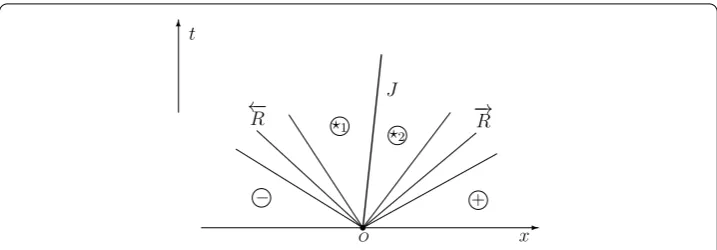
divide the (ρ,u)-plane into five regions, as shown in Figure .
When the projection of the state (ρ+,u+,H+) onto the (ρ,u)-plane lies inI∪II∪III∪IV,
namely,u–– √
Aρ–(+α)/ – <u++
√
Aρ+–(+α)/, the Riemann problem can be solved in the
following way. On the physically relevant regionℵ, we draw the backward wave curve
←–
R(ρ–,u–,H–) or←
–
S(ρ–,u–,H–), and the forward wave curve
–
→
R(ρ+,u+,H+) or
–
→
S(ρ+,u+,H+).
The projections of these curves onto the (ρ,u)-plane have a unique intersection point (ρ,u). Then we draw the contact discontinuity curveJ(ρ,u,H–), which intersects the
backward and forward wave curves at the unique points (ρ,u,H) and (ρ,u,H).
Figure 2 The structure of solution as the projection of state +onto (ρ,u)-plane lies inI.
Figure 3 The structure of solution as the projection of state +onto (ρ,u)-plane lies inII.
Figure 4 The structure of solution as the projection of state +onto (ρ,u)-plane lies inIII.
Hence, we obtain four kinds of exact solutions, as shown in Figures -. The conclusion is stated by the following theorem.
Theorem On the physically relevant regionℵ,under the condition u–– √
Aρ–(+α)/ – <
u++ √
Aρ+–(+α)/,the Riemann problem(.), (.),and(.)admits four kind of exact
Figure 5 The structure of solution as the projection of state +onto (ρ,u)-plane lies inIV.
Figure 6 The characteristic lines whenu––
√
Aρ–(1+α)/2 – ≥u++
√
Aρ–(1+α)/2
+ .
3 Delta shock wave solution
3.1 Delta shock wave with Dirac delta function in both density and internal energy
We solve the Riemann problem (.), (.), and (.) when the projection of the state (ρ+,u+,H+) onto the (ρ,u)-plane lies inV, namely,
u–– √
Aρ––(+α)/≥u++ √
Aρ+–(+α)/. (.)
The characteristic line defined byx/t=λi,i= , , from the initial data will overlap in the
domainΩ={(t,x)|(u++ √
Aαρ+–(+α)/)t≤x≤(u–– √
Aαρ–(+α)/
– )t, ≤t< +∞}, as
illus-trated in Figure . Hence, the singularity will develop inΩ, while this singularity cannot be a jump with finite amplitudes.
To analyze the singularity in Ω, we first study the special case u– – √
Aρ––(+α)/ = u++
√
Aρ+–(+α)/. Let us consider the limit of the solutionρ(ξ),u(ξ), andH(ξ) whenρ–,u–,
H–,ρ+,H+are fixed,u+→u–– √
A(ρ–(α+)/
– +ρ
–(α+)/
+ ) + . Whenu+>u–– √
A(ρ–(α+)/
– +
ρ+–(α+)/) and the projection of the state (ρ+,u+,H+) on the (ρ,u)-plane lies inIII, the
so-lution is depicted in Figure , where
⎧ ⎪ ⎨ ⎪ ⎩
ρ=ρ=ρ, u=u=u, H=
A(ρ–
α
– +ρ–α) + ρ
ρ–(H––
A(ρ–
α
– +ρ–α)),
H=
A(ρ–
α
+ +ρ–α) + ρ
ρ+(H+–
A(ρ–
α
+ +ρ–α)),
andu,ρare uniquely determined by ⎧ ⎪ ⎨ ⎪ ⎩
u=u––
A(ρ–α – –ρ–α)
ρρ–(ρ–ρ–)(ρ–ρ–), ρ>ρ–, u=u++
A(ρ+–α–ρ–α)
ρρ+(ρ–ρ+)(ρ–ρ+), ρ>ρ+.
(.)
From (.), one shows that
u+=u––
A(ρ–α
– –ρ–α)
ρρ–(ρ–ρ–)
(ρ–ρ–) –
A(ρ–α
+ –ρ–α)
ρρ+(ρ–ρ+)
(ρ–ρ+)
=u–– √
Aρ– – –ρ–
ρ–α
– –ρ–α
–√Aρ– + –ρ–
ρ–α
+ –ρ–α
. (.)
Besides, according to (.), one obtains that
H––
Aρ
–α
– >H––
A +αρ
–α
– ≥, H+–
Aρ
–α
+ >H+–
A +αρ
–α
+ ≥. (.)
Thus, asu+→u–– √
A(ρ––(α+)/+ρ+–(α+)/) + , the combination of (.)-(.) yields
ρ=ρ=ρ→ ∞, H→ ∞, H→ ∞, u=u=u→u++
√
Aρ–(+α+)/=u–– √
Aρ–(α+)/
– ,
(.)
and then←S–,Jand→–S coincide to form a new singularity.
Let us calculate the total quantities ofρ,uandHbetween←S–and→–S asρ–,u–,H–,ρ+,H+
are fixed,u+→u–– √
A(ρ–(α+)/
– +ρ
–(α+)/
+ ) + , and the projection of the state (ρ+,u+,H+)
on the (ρ,u)-plane lies inIII,
lim
u+→u––√A(ρ––(α+)/+ρ–(+α+)/)+
u+(Aρ–(ρ–ρ+)–ρ+(ρ–+α–ρ–α))/
u–(Aρ– (ρ–ρ–)–ρ–(ρ–α – –ρ–α))/
ρ(ξ) dξ
= lim
u+→u––
√
A(ρ––(α+)/+ρ+–(α+)/)+
u+(Aρ– (ρ–ρ+)–ρ+(ρ+–α–ρ–α))/
u–(Aρ–(ρ–ρ–)–ρ–(ρ–α – –ρ–α))/
ρdξ
= lim
ρ→∞
ρ
Aρ+(ρ
–α
+ –ρ–α)
ρ(ρ–ρ+)
+
Aρ–(ρ
–α
– –ρ–α)
ρ(ρ–ρ–)
=√Aρ–(–α)/+ρ+(–α)/
= , (.)
lim
u+→u––
√
A(ρ–(–α+)/+ρ–(+α+)/)+
u+(Aρ–(ρ–ρ+)–ρ+(ρ–+α–ρ–α))/ u–(Aρ– (ρ–ρ–)–ρ–(ρ–α
– –ρ–α))/
u(ξ) dξ
= lim
u+→u––√A(ρ––(α+)/+ρ+–(α+)/)+
u+(Aρ– (ρ–ρ+)–ρ+(ρ+–α–ρ–α))/
u–(Aρ–(ρ–ρ–)–ρ–(ρ–α – –ρ–α))/
udξ
= lim
ρ→∞ u
Aρ+(ρ
–α
+ –ρ–α)
ρ(ρ–ρ+)
+
Aρ–(ρ
–α
– –ρ–α)
ρ(ρ–ρ–)
lim
u+→u––√A(ρ––(α+)/+ρ–(+α+)/)+
u+(Aρ–(ρ–ρ+)–ρ+(ρ–+α–ρ–α))/
u–(Aρ– (ρ–ρ–)–ρ–(ρ–α – –ρ–α))/
H(ξ) dξ
= lim
u+→u––√A(ρ––(α+)/+ρ+–(α+)/)+
u
u–(Aρ–(ρ–ρ–)–ρ–(ρ–α – –ρ–α))/
Hdξ
+
u+(Aρ–(ρ–ρ+)–ρ+(ρ+–α–ρ–α))/
u
Hdξ
= lim
ρ→∞
H
Aρ–(ρ
–α
– –ρ–α)
ρ(ρ–ρ–)
+H
Aρ+(ρ
–α
+ –ρ–α)
ρ(ρ–ρ+)
=√A
ρ––(+α)/
H––
A ρ
–α
–
+ρ+–(+α)/
H+–
A ρ
–α
+
= . (.)
Equations (.)-(.) show thatρ(ξ) andH(ξ) have the same singularity as a weighed Dirac delta function atξ=u––
√
Aρ–(α+)/
– , and thatu(ξ) has a bounded variation. Thus, the
singularity inΩis a delta shock wave with a Dirac delta function in bothρandH. Besides, the inequality
λ(ρ+,u+) <λ(ρ+,u+) <λ(ρ+,u+) <σ<λ(ρ–,u–) <λ(ρ–,u–) <λ(ρ–,u–),
holds, whereσ=u–– √
Aρ–(α+)/ – =u++
√
Aρ+–(α+)/is the velocity of the delta shock wave.
It means that none of the six characteristic lines on both sides of the delta shock wave is outgoing.
By the above analysis, for the general caseu–– √
Aρ–(+α)/
– ≥u++
√
Aρ+–(+α)/, the delta
shock wave solution which contains a Dirac delta function in bothρandHis suggested. We first give two definitions.
Definition The two-dimensional weighted delta functionw(s)δLsupported on a smooth
curveLparameterized asx=x(s),y=y(s) (c≤s≤d) is defined as
w(s)δL,φ(x,y)
=
d
c
w(s)φx(s),y(s)ds, (.)
for all the test functionsφ∈C∞(R).
Definition The triple distribution (ρ,u,H) is a delta shock wave solution of (.) and (.) in the sense of distribution if there exist a smooth curveLand two functions w(t),h(t)∈C(L) such thatρ,u,Hare of the following form:
ρ=ρ¯(t,x) +w(t)δL, u=u¯(t,x), H=H¯(t,x) +h(t)δL, (.)
and
⎧ ⎪ ⎨ ⎪ ⎩
ρ,φt+ρu,φx= ,
ρu,φt+ρu+p,φx= ,
ρu/ +H,φ
t+(ρu/ +H+p)u,φx= ,
for all the test functionsφ∈C∞((, +∞)×R), whereρ¯,u¯,H¯ ∈L∞([, +∞)×R;R),u|L= uδ(t),
ρ,φ=
+∞
+∞
–∞ ¯
ρ(t,x)φdxdt+w(t)δL,φ
,
ρu,φ=
+∞
+∞
–∞ ¯
ρu¯(t,x)φdxdt+w(t)uδ(t)δL,φ
,
andHhas the similar integral identities as above.
With Definitions -, we seek a delta shock wave solution with the discontinuityx=x(t) to (.) and (.) in the form
(ρ,u,H)(t,x) =
⎧ ⎪ ⎨ ⎪ ⎩
(ρ–,u–,H–), x<x(t),
(w(t)δ(x–x(t)),uδ(t),h(t)δ(x–x(t))), x=x(t),
(ρ+,u+,H+), x>x(t),
(.)
where (ρi,ui,Hi),i= –, + are smooth bounded solutions to (.) and (.),δis the standard
Dirac measure supported on the curvex(t), andw(t),h(t) are the weights of the delta shock wave on the state variablesρ,H. Besides, we define
p= ⎧ ⎪ ⎨ ⎪ ⎩
–Aρ––α, x<x(t),
, x=x(t),
–Aρ–α
+ , x>x(t).
(.)
Lemma If the solution of the form (.) satisfies the following generalized Rankine-Hugoniot relation:
⎧ ⎪ ⎪ ⎪ ⎪ ⎪ ⎨ ⎪ ⎪ ⎪ ⎪ ⎪ ⎩ dx(t) dt =uδ(t), dw(t)
dt =uδ(t)[ρ] – [ρu],
d(w(t)uδ(t))
dt =uδ(t)[ρu] – [ρu +p], d(w(t)uδ(t)/+h(t))
dt =uδ(t)[ρu/ +H] – [(ρu/ +H+p)u],
(.)
then it is a delta shock wave solution to(.)and(.)in the sense of distribution.
Proof If equation (.) holds, then, for any test functionsφ∈C∞((, +∞)×R), by Green’s formulation and integrating by parts, we obtain
ρu/ +H,φt
+ρu/ +H+pu,φx = +∞ +∞ –∞
ρu/ +Hφt+
ρu/ +H+puφxdxdt
+
+∞
w(t)uδ(t)/ +h(t)
φt+
w(t)uδ(t)/ +h(t)
uδ(t)
φxdt
= +∞ x(t) –∞
ρ–u–/ +H–
φt+ρ–u–/ +H–+p–
u–φ
xdxdt
+ +∞ +∞ x(t)
ρ+u+/ +H+
φt+ρ+u+/ +H++p+
u+φ
+
+∞
w(t)uδ(t)/ +h(t)
φt+uδ(t)φx
dt
= –
+∞
–ρ–u–/ +H–+p–
u–φ
dt+ρ–u–/ +H–
φdx
+
+∞
–ρ+u+/ +H++p+
u+φ
dt+ρ+u+/ +H+
φdx
–
+∞
φd(w(t)u
δ(t)/ +h(t))
dt dt
=
+∞
φ
uδ(t)
ρu/ +H–ρu/ +H+pu– d(w(t)u
δ(t)/ +h(t))
dt
dt
= , (.)
which yields the third equality of (.). In a similar way, one can prove the first and second
equalities of (.). The proof is complete.
Remark The generalized Rankine-Hugoniot equation (.) describes the exact rela-tionship between the limit states on two sides of a delta shock wave and the location, speed, weights, and the assignments ofuon the delta shock wave.
In addition, to guarantee the uniqueness of delta shock wave solution, we propose the following entropy condition for a delta shock wave:
λ(ρ+,u+) <λ(ρ+,u+) <λ(ρ+,u+)≤uδ(t)≤λ(ρ–,u–)
<λ(ρ–,u–) <λ(ρ–,u–), (.)
which means that all of the six characteristic lines on both sides of the delta shock wave are incoming.
Definition The discontinuity satisfying (.) and (.) is called a delta shock wave, denoted byδ.
3.2 Solution involving delta shock wave
In this subsection, both the generalized Rankine-Hugoniot relation and the entropy condi-tion for the delta shock wave will be applied to solve the Riemann problem (.), (.), and (.) whenu––
√
Aρ––(+α)/≥u++ √
Aρ+–(+α)/. At this moment, this Riemann problem is
reduced to the initial value problem for (.) and (.) with the initial conditions
x() = , uδ() = , w() = , h() = . (.)
From (.) and (.), it leads to
⎧ ⎪ ⎨ ⎪ ⎩
w(t) =x(t)[ρ] – [ρu]t,
w(t)uδ(t) =x(t)[ρu] – [ρu+p]t,
w(t)u
δ(t)/ +h(t) =x(t)[ρu/ +H] – [(ρu/ +H+p)u]t.
We multiply the first equation of (.) byuδ(t) and then subtract it from the second
equa-tion to obtain
[ρ]x(t)uδ(t) – [ρu]x(t) – [ρu]uδ(t)t+
ρu+pt= ,
or
d dt
[ρ]x(t)/ – [ρu]x(t)t+ρu+pt/= ,
that is,
[ρ]x(t) – [ρu]x(t)t+ρu+pt= . (.)
When [ρ] =ρ+–ρ–= , we can deduce that
⎧ ⎪ ⎪ ⎪ ⎨ ⎪ ⎪ ⎪ ⎩
x(t) = (u–+u+)t/,
uδ(t) = (u–+u+)/,
w(t) =ρ–(u––u+)t,
h(t) = –w(t)uδ(t)/ +x(t)[ρu/ +H] – [(ρu/ +H+p)u]t,
(.)
which satisfies the entropy condition (.).
When [ρ] =ρ+–ρ–= , noting (.), the discriminant of the quadratic equation (.)
holds,
Δ= t[ρu]– [ρ]ρu+p
= tρ–ρ+[u]+A(ρ+–ρ–)
ρ+–α–ρ––α
= tρ+ρ–
[u]–Aρ–––ρ+–ρ––α–ρ+–α
> .
Therefore, (.) admits two solutions
x(t) =
t [ρ]
[ρu] +[ρu]– [ρ]ρu+p/, (.)
x(t) =
t [ρ]
[ρu] –[ρu]– [ρ]ρu+p/. (.)
Let us single out an admissible solution from (.) and (.) using the entropy condi-tion (.). For the solucondi-tion (.), it shows that
uδ(t) =x(t) =
[ρ]
[ρu] +[ρu]– [ρ]ρu+p/. (.)
Then, by using (.) and noting
[ρu]– [ρ]ρu+p–√Aαρ+–(+α)/[ρ] –ρ–[u]
=[ρu]– [ρ]ρu+p–ρ–
u––
u++ √
= [ρ]ρ–
u++ √
Aαρ+–(+α)/–u–+ √
Aρ––(+α)/u++ √
Aαρ+–(+α)/
–u–– √
Aρ––(+α)/+A( –α)ρ–+α, (.)
–ρ+[u] – √
Aαρ––(+α)/[ρ]–[ρu]– [ρ]ρu+p =ρ+
u–– √
Aαρ––(+α)/–u+
+√Aαρ––(+α)/–[ρu]– [ρ]ρu+p = [ρ]ρ+
u++ √
Aρ+–(+α)/–u–– √
Aαρ––(+α)/u+– √
Aρ–(++ α)/
–u–– √
Aαρ––(+α)/+A( –α)ρ––α, (.)
we can deduce that
uδ(t) –
u++ √
Aαρ+–(+α)/
=
[ρ]
[ρu]– [ρ]ρu+p/–√Aαρ+–(+α)/[ρ] –ρ–[u]
> , (.)
u–– √
Aαρ––(+α)/–uδ(t)
=
[ρ]
–ρ+[u] – √
Aαρ–(+– α)/[ρ]–[ρu]– [ρ]ρu+p/
> , (.)
namely,u++ √
Aαρ+–(+α)/<uδ(t) <u–– √
Aαρ––(+α)/. However, for the solution (.), it is easy to see that
uδ(t) =x(t) =
[ρ]
[ρu] –[ρu]– [ρ]ρu+p/. (.)
As [ρ] > , a combination of (.), (.), and (.) shows that
uδ(t) –
u++ √
Aαρ+–(+α)/
=
[ρ]
–[ρu]– [ρ]ρu+p/–√Aαρ+–(+α)/[ρ] –ρ–[u]
< , (.)
u–– √
Aαρ––(+α)/–uδ(t)
=
[ρ]
–ρ+[u] – √
Aαρ–(+– α)/[ρ]–[ρu]+ [ρ]ρu+p/
> , (.)
that is,uδ(t) <u++ √
Aαρ+–(+α)/<u–– √
Aαρ–(+α)/
– . By the entropy condition (.), we
choose (.) as an admissible solution. Thus, from (.), we obtain
⎧ ⎪ ⎪ ⎪ ⎨ ⎪ ⎪ ⎪ ⎩
x(t) =[ρ]([ρu]t+w(t)), uδ(t) =[ρ]([ρu] +w(t)),
w(t) = ([ρu]– [ρ][ρu+p])/t, h(t) = –w(t)u
δ(t)/ +x(t)[ρu/ +H] – [(ρu/ +H+p)u]t.
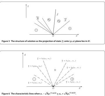
Figure 7 The structure of solution as the projection of state +onto (ρ,u)-plane lies inV.
According to (.) and (.), with a simple calculation, we obtain the following proper-ties of the solution to (.) and (.).
Lemma On the physically relevant regionℵ,under the condition u–– √
Aρ–(+α)/
– ≥
u++ √
Aρ+–(+α)/,the solution to(.)and(.)has the following properties.
(i) x(t)is a monotone function oft. (ii) uδ(t)is a constant value,satisfyingu++
√
Aαρ+–(α+)/<uδ(t) <u–– √
Aαρ––(α+)/. (iii) w(t)≥is a monotone increasing function oft.
(iv) h(t)≥is a monotone increasing function oft.
Therefore, we have the following result.
Theorem On the physically relevant regionℵ,under the condition u–– √
Aρ––(+α)/≥
u++ √
Aρ+–(+α)/,the Riemann problem(.), (.)and(.)admits uniquely a delta shock
wave solution of the form
(ρ,u,H)(t,x) =
⎧ ⎪ ⎨ ⎪ ⎩
(ρ–,u–,H–), x<x(t),
(w(t)δ(x–x(t)),uδ(t),h(t)δ(x–x(t))), x=x(t),
(ρ+,u+,H+), x>x(t),
(.)
where x(t),uδ(t),w(t),and h(t)are shown in(.)forρ–=ρ+or(.)forρ–=ρ+.See
Figure.
3.3 Numerical simulation to the delta shock wave solution
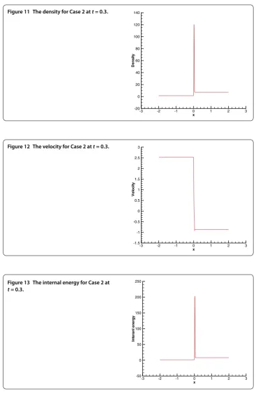
This subsection gives some numerical simulations for the delta shock wave solution men-tioned above. In the following examples, we takeA= .,α= ., and the interval [–, ], and compute the solution using the Nessyahu-Tadmor scheme [] with CFL = ..
Case.u–– √
Aρ–(+α)/ – =u++
√
Aρ+–(+α)/. The initial data are as follows:
ρ–= ., u–= ., H–= .,
ρ+= ., u+= ., H+= .,
(.)
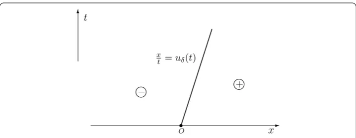
Figure 8 The density for Case 1 att= 0.3.
Figure 9 The velocity for Case 1 att= 0.3.
Figure 10 The internal energy for Case 1 at t= 0.3.
Case.u–– √
Aρ–(+α)/ – >u++
√
Aρ–(++ α)/. The initial data are as follows:
ρ–= ., u–= ., H–= .,
ρ+= ., u+= –., H+= .,
(.)
Figure 11 The density for Case 2 att= 0.3.
Figure 12 The velocity for Case 2 att= 0.3.
Figure 13 The internal energy for Case 2 at t= 0.3.
From Figures and or Figures and , it is clearly observed that both densityρ
4 Conclusion
In this study, we completely solve the Riemann problem for the compressible Euler equa-tions with the generalized Chaplygin gas. Its soluequa-tions exhibit five kinds of geometrical structures. It is shown that the delta shock wave with Dirac delta function in both den-sity and internal energy develops in the solutions. To our knowledge, this type of delta shock wave has not been found in the previous investigations of the generalized Chaplygin gas. Besides, the formation mechanism of this kind of delta shock wave in the generalized Chaplygin gas results from the overlapping of the linearly degenerate and genuinely non-linear characteristic lines, which is substantially different from the case of the Chaplygin gas.
Competing interests
The author declares that there are no competing interests regarding the publication of this paper.
Acknowledgements
The author is grateful to the anonymous referees for his/her valuable comments and corrections, which helped to improve the manuscript. This work is partially supported by the National Natural Science Foundation of China (11526063, 11661015), the Natural Science Foundation of the Education Department of Guizhou Province (KY[2015]482), the Science and Technology Foundation of Guizhou Province (J[2015]2026) and the Project of High Level Creative Talents in Guizhou Province (20164035).
Received: 13 May 2016 Accepted: 8 November 2016 References
1. Lax, PD: Hyperbolic Systems of Conservation Laws and the Mathematical Theory of Shock Waves. SIAM, Philadelphia (1973)
2. Chang, T, Hsiao, L: The Riemann Problem and Interaction of Waves in Gas Dynamics. Longman, Harlow (1989) 3. Chen, GQ, Liu, H: Formation of delta-shocks and vacuum states in the vanishing pressure limit of solutions to the
Euler equations for isentropic fluids. SIAM J. Math. Anal.34, 925-938 (2003)
4. Chen, GQ, Liu, H: Concentration and cavitation in the vanishing pressure limit of solutions to the Euler equations for nonisentropic fluids. Physica D189, 141-165 (2004)
5. Chaplygin, S: On gas jets. Sci. Mem. Mosc. Univ. Math. Phys.21, 1-121 (1904)
6. Tsien, HS: Two-dimensional subsonic flow of compressible fluids. J. Aeronaut. Sci.6, 399-407 (1939) 7. Kamenshchik, AY, Moschella, U, Pasquier, V: An alternative to quintessence. Phys. Lett. B511, 265-268 (2001) 8. Bento, MC, Bertolami, O, Sen, AA: Generalized Chaplygin gas, accelerated expansion, and dark-energy-matter
unification. Phys. Rev. D66, 043507 (2002)
9. Bento, MC, Bertolami, O, Sen, AA: Generalized Chaplygin gas model: dark energy-dark matter unification and cmbr constraints. Gen. Relativ. Gravit.35, 2063-2069 (2003)
10. Bilic, N, Tupper, GB, Viollier, RD: Unification of dark matter and dark energy: the inhomogeneous Chaplygin gas. Phys. Lett. B535, 17-21 (2002)
11. Brenier, Y: Solutions with concentration to the Riemann problem for one-dimensional Chaplygin gas equations. J. Math. Fluid Mech.7, S326-S331 (2005)
12. Guo, L, Sheng, W, Zhang, T: The two-dimensional Riemann problem for isentropic Chaplygin gas dynamic system. Commun. Pure Appl. Anal.9, 431-458 (2010)
13. Tan, D, Zhang, T, Zheng, Y: Delta-shock waves as limits of vanishing viscosity for hyperbolic systems of conservation laws. J. Differ. Equ.112, 1-32 (1994)
14. Yang, H, Zhang, Y: New developments of delta shock waves and its applications in systems of conservation laws. J. Differ. Equ.252, 5951-5993 (2012)
15. Wang, G: The Riemann problem for one dimensional generalized Chaplygin gas dynamics. J. Math. Anal. Appl.403, 434-450 (2013)
16. Sheng, W, Wang, G, Yin, G: Delta wave and vacuum state for generalized Chaplygin gas dynamics system as pressure vanishes. Nonlinear Anal., Real World Appl.22, 115-128 (2015)
17. Sun, M: The exact Riemann solutions to the generalized Chaplygin gas equations with friction. Commun. Nonlinear Sci. Numer. Simul.36, 342-353 (2016)
18. Kraiko, AN: Discontinuity surfaces in medium without self-pressure. Prikl. Math. Mech.43, 539-549 (1979) 19. Nilsson, B, Rozanova, OS, Shelkovich, VM: Mass, momentum and energy conservation laws in zero-pressure gas
dynamics and delta-shocks: II. Appl. Anal.90, 831-842 (2011)
20. Nilsson, B, Shelkovich, VM: Mass, momentum and energy conservation laws in zero-pressure gas dynamics and delta-shocks. Appl. Anal.90, 1677-1689 (2011)
21. Cheng, H: Riemann problem for one-dimensional system of conservation laws of mass, momentum and energy in zero-pressure gas dynamics. Differ. Equ. Appl.4, 653-664 (2012)
22. Shelkovich, VM: Delta-shock waves in nonlinear chromatography. In: 13th International Conference on Hyperbolic Problems: Theory, Numerics, Applications, Xijiao Hotel, Beijing, 15-19 June, pp. 15-19 (2010)
24. Cheng, H, Yang, H: Delta shock waves in chromatography equations. J. Math. Anal. Appl.380, 475-485 (2011) 25. Yang, H, Zhang, Y: Delta shock waves with Dirac delta function in both components for systems of conservation laws.
J. Differ. Equ.257, 4369-4402 (2014)
26. Zhu, L, Sheng, W: The Riemann problem of adiabatic Chaplygin gas dynamic system. Commun. Appl. Math. Comput. 24, 9-16 (2010)