R E S E A R C H
Open Access
Identifying an unknown source in the Poisson
equation by a wavelet dual least square
method
Ai-lin Qian
**Correspondence:
[email protected] Department of Mathematics and Statistics, Hubei University of Science and Technology, Xianning, Hubei 437100, People’s Republic of China
Abstract
This paper deals with an inverse problem of identifying an unknown source which depends only on one variable in two-dimensional Poisson equation, with the aid of an extra measurement at an internal point. This problem is ill-posed, we proposed a regularization strategy, a wavelet dual least square method, to analyze the stability of the problem. Meanwhile, a numerical experiment is devised to verify the validity of the method.
MSC: 35R40; 65J20
Keywords: ill-posed problems; Meyer wavelet; regularization; dual least square method; error estimate
1 Introduction
Consider the following inverse problem: find a pair of functions (u(x,y),f(x)) satisfying
⎧ ⎪ ⎪ ⎪ ⎪ ⎪ ⎨ ⎪ ⎪ ⎪ ⎪ ⎪ ⎩
–uxx–uyy=f(x), –∞<x<∞,y> ,
u(x, ) = , –∞<x<∞,
u(x,y)|y→∞bounded, –∞<x<∞,
u(x, ) =g(x), –∞<x<∞,
(.)
wheref(x) is the unknown source depending only on one spatial variable andu(x, ) =g(x) is the supplementary condition. In practical applications, the input datag(x) can only be measured. There will be measured data functiongδ(x) which is merely inL(R) and satisfies
g–gδL(R)≤δ, (.)
where the constantδ> represents a noise level of input data. This problem is called the inverse problem of unknown source identification.
Inverse source identification problems are important in many branches of engineering sciences such as crack determination [, ], heat source determination [], heat conduction problems [, ], electromagnetic theory []. This kind of problem arises in many important applications in practice,e.g., with the development of society and economics, groundwa-ter pollution has become a serious threat to the environment. The government has to take
some measures to prevent the groundwater from further contaminations. But the cost of cleanup for polluted aquifers is staggering, and in many cases it is hard to identify which companies are responsible for the contamination due to the lack of tools to discover the pollution sources. So, it is necessary to try to give more concrete information of the charac-teristics (location, magnitude, and duration of activity) of specific groundwater pollution sources (see []). As we know, most attempts at quantifying contaminant transport rely on mathematical methods. Since the data cannot be measured by direct ways in many cases, we are always encountering inverse problems of deciding unknown sources and aquifer parameters.
The investigation of the traditional inverse potential problem can be found in [, ]. The studies of such problems give a complete analysis of experimental data. In general, a full sourcef in (.) is not solely attainable from boundary measurements. The inverse source identification problem becomes solvable if somea prioriknowledge is assumed. For in-stance, when one of the products in the separation of variables is known [, ], or the base area of a cylindrical source is known [], or a non-separable type is in the form of a mov-ing front [], the boundary datag can then uniquely determine the unknown sourcesf. Furthermore, when bothuandfare relatively smooth, some standard regularization tech-niques can be employed (see [] for a more detailed overview).
Wavelet regularization methods have been studied for solving various types of inverse problems in the heat equation [–]. Eldén [] and Regińska [, ], Xiong [] used the wavelet Galerkin method and the wavelet method to approximate the sideways heat equation by Meyer wavelets, and Xiong [] used the wavelet dual least squares method to approximate the BHCP by Shannon wavelets. In this work, by using Meyer wavelets, we obtain an explicit error estimate of Hölder type between the unknown source term and its approximation. Moreover, according to the general theory of regularization, we conclude that our estimate is order optimal.
In general, for an ill-posed problem, the convergence rates of the regularization solution can only be given undera prioriassumptions on the exact data. We will formulate such ana prioriassumption in terms of an exact solutionf(x) by considering
fp≤E, p> , (.)
where the · pdenotes the Sobolev spaceHp(R)-norm defined by
fp:=
∞
–∞
+ξ pfˆ(ξ)dξ /
. (.)
In order to formulate problem (.) in terms of an operator equation in the spaceX= L(R), letAbe the operator onXdefined as follows:
Af(x) =g(x). (.)
Let
ˆ
f(ξ) =√ π
∞
–∞f(x)e
be the Fourier transform of the functionf(x)∈L(R). Problem (.) can now be formulated in a frequency space as follows:
⎧ ⎪ ⎪ ⎪ ⎪ ⎪ ⎨ ⎪ ⎪ ⎪ ⎪ ⎪ ⎩
ξuˆ(ξ,y) –uˆ
yy(ξ,y) =fˆ(ξ), –∞<x<∞,y> ,
ˆ
u(ξ, ) = , –∞<x<∞,
ˆ
u(ξ,y)|y→∞bounded, –∞<x<∞,
ˆ
u(ξ, ) =gˆ(ξ), –∞<x<∞.
(.)
By elementary calculations, the solution of problem (.) in the frequency space is given by
ˆ
f(ξ) = ξ
–e–ξgˆ(ξ), (.)
which shows thatAˆ :L(R)→L(R) is the multiplication operator. In addition,Aˆ is self-adjoint,i.e.,
ˆ
A∗fˆ=Aˆˆf= –e –ξ
ξ gˆ(ξ). (.)
2 Preliminaries
2.1 Dual least squares method
A general projection method for the operator equationAf=g,A:X=L(R) −→X=L(R) is generated by two subspace families{Vj}and{Yj}ofX, and the approximate solution
fj∈Vjis defined to be the solution of the following problem:
Afj,y=g,y, ∀y∈Yj, (.)
where·,·denotes the inner product inX. IfVj⊂R(A∗) and subspacesYjare chosen such
that
A∗Yj=Vj, (.)
then we have a special case of the projection method known as the dual least squares method. If{ψλ}λ∈Ijis an orthogonal basis ofVjandyλis the solution of the equation
A∗yλ=kλψλ, yλ= , (.)
then the approximate solution is explicitly given by the expression
fj=
λ∈Ij g,yλ
kλ
ψλ. (.)
2.2 SubspacesYj
In this section, we investigate some properties of the subspacesYj. A method for
con-structing the basis of the subspace is given. This method is different from [] in that the functionv(ξ,y) is not specific. The basis ofYjcannot be explicitly obtained by dilations
According toA∗Yj=Vj, the subspacesYjare spanned byfλ,λ∈Ij, where
A∗fλ=λ and kλ=fλ–, yλ= fλ
fλ
=kλfλ. (.)
Sincesuppˆλis compact, the solution exists for anyy∈[, ). Similarly, the solution of the adjoint problem is unique. Therefore, for a givenλ,fλcan be uniquely determined; furthermore,
ˆ
fλ=v(ξ,y)ˆλ(ξ) ⇔ ˆyλ=v(ξ,y)kλˆλ(ξ), λ={j,k}. (.)
As for some properties ofkλ, the results are similar to Lemma . of []. Here we omit it.
2.3 Meyer wavelets
The Meyer waveletψis a functionC∞(R) defined by its Fourier transform as follows []:
ˆ ψ(ξ) =
⎧ ⎪ ⎪ ⎨ ⎪ ⎪ ⎩ √ πe
iξsin[π ν(
π|ξ|– )], π
≤ |ξ| ≤ π
,
√ πe
iξcos[π ν(
π|ξ|– )], π
≤ |ξ| ≤ π
,
, otherwise,
(.)
whereν∈Ck is equal to forx≤, is equal to forx≥, andν(x) +ν( –x) = for <x< . The corresponding scaling functionφis defined by
ˆ φ(ξ) =
⎧ ⎪ ⎪ ⎨ ⎪ ⎪ ⎩
π, |ξ| ≤ π , √ πcos[ π ν(
π|ξ|– )], π
≤ |ξ| ≤ π
, , otherwise.
(.)
Let us list some notations:ψj,k(x) :=
j
ψ(jx–k),φj,k(x) := j
φ(jx–k),j,k∈Z;–,k:= φ,kandl,k:=ψl,kforl≥; wavelet spacesWj=span{ψj,k}j,k∈Z; some index sets (where
J≥ is a fixed integer)
I={j,k}:j,k∈Z⊂Z,
IJ=
{j,k}:j= –, , . . . ,J– ;k∈Z⊂Z, (.)
Ij≥J+=
{j,k}:j≥J;k∈Z⊂Z.
By successively decomposing the scaling spaceVJ,VJ–and so on, we haveVJ =VJ–⊕ WJ–=VJ–⊕WJ–⊕WJ–=· · ·=V⊕W⊕ · · · ⊕WJ–, hence we can define the
sub-spacesVJ
VJ=span{λ}λ∈IJ. (.)
Define an orthogonal projectionPJ:L(R) −→VJ:
PJϕ=
λ∈IJ
then replace the{ψλ}λ∈Ijin (.) by{λ}λ∈IJ. We easily conclude
fJ=PJf. (.)
From the point of view of an application to problem (.), the important property of Meyer wavelets is the compactness of their support in the frequency space. Indeed, since
ˆ
ψj,k(ξ) = –
j
e–i–jkξψˆ–jξ , φˆ
j,k(ξ) = –
j
e–i–jkξφˆ–jξ ,
it follows that for anyk∈Z,
supp(ψˆj,k) =
ξ:
π
j≤ |ξ| ≤
π
j
, supp(φˆj,k) =
ξ:|ξ| ≤
π
j
. (.)
From (.),PJcan be seen as a low pass filter. The frequencies with greater thanπJare
filtered away.
3 Error estimates for the wavelet dual least square method
Theorem . If f(x)is the solution of problem(.)satisfying condition(.),then it holds
that
f(·) –PJf(·)≤
π
J+
–p
E. (.)
Proof From (.), we have
f(·) = λ∈I
f(·),λ
λ,
PJf(·) =
λ∈IJ
f(·),λ
λ.
By virtue of the Parseval relation, with theˆλ’s compact support (.), there holds
f(·) –PJf(·)=ˆf(·) –PJf(·)=
λ∈I
ˆf,ˆλ ˆλ–
λ∈IJ
ˆf,ˆλ ˆλ
= λ∈Ij≥J+
ˆf,ˆλ ˆλ
= λ∈Ij≥J+
+ξ –p/ +ξ p/fˆ(·),ˆλ
ˆ λ ≤ sup
πj+≤|ξ|≤πj+
+ξ –p/| ·
λ∈Ij≥J+
+ξ p/fˆ(·),ˆλ
ˆ λ ≤ π
J+
–p
The approximate solution for noisy datagδis explicitly given by
PJfδ(x) =fJδ=
λ∈IJ
fδ, λ
λ=
λ∈IJ gδ,yλ
kλ
λ. (.)
Now we will estimate the errorPJfδ–PJf.
Theorem . If gδis noisy data satisfying condition(.),then for any fixed y,we have
PJfδ–PJf≤C
π
J+
δ, C= –e–π
.
= . (.)
Proof Using (.), (.), and (.), from the Parseval relation, we have
PJfδ–PJf
= λ∈IJ
–λ
ˆ
gδ–gˆ,
ξ –e–ξkλˆλ
ˆ λ ≤ sup
πJ≤|ξ|≤πJ ξ –e–ξ
λ∈IJ
(gˆδ–gˆ,ˆλ)ˆλ
≤ sup
πJ≤|ξ|≤πJ ξ
–e–ξPJ(gδ–g)
≤ sup
πJ≤|ξ|≤πJ ξ
–e–ξ(gδ–g)
≤ (
πJ) –e–πJδ
≤C
π
J+
δ, C= –e–π
.
= .
Theorem . If f(·)is the solution of problem(.)satisfying the conditionu(·, )p≤E,
let PJfδbe given by(.).Ifg–gδ ≤δand J=J(δ)is selected such that
π
J+=
E δ p+ , (.) then
f(·) –PJfδ
(·)≤(C+ )Ep+ δ p
p+. (.)
Proof By the triangle inequality, we have
f(·) –PJfδ(·)≤f(·) –PJf(·)+PJf(·) –PJfδ(·). (.)
Combining Theorem . with Theorem ., we obtain the convergence estimate of our
4 Numerical tests
Example It is easy to see that the function
u(x,y) = –e–y sinx (.)
and the function
f(x) =sinx (.)
satisfy problem (.) with exact data
g(x) = –e– sinx. (.)
We will do the numerical tests in the intervalx∈[–, ].
Suppose that the sequence g(xi)ni= represents samples from the functiong(x) on an equidistant grid, andnis even, then we add a random uniformly distributed perturbation to each data, and obtain the perturbation data
gδ=g+μ∗rand
size(g) , (.)
where
g=g(x),g(x), . . . ,g(xn), xi= (i– )x– ,x=
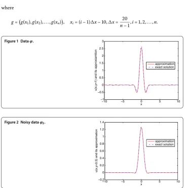
n– ,i= , , . . . ,n.
Figure 1 Dataϕ.
Then the total noiseδcan be measured in the sense of root mean square error according to
δ=gδ–gl=
n
n
i=
(gδ)i–gi
/
. (.)
The computed errors are defined by
lnorm error:E(f) =
n
n
i=
f(xi) –fr(xi)
, (.)
relative error:ER(f) =
n
n
i=
f(xi) –fr(xi)
n
n
i=
(f(xi), (.)
wherexi,i= , , . . . ,n, are the test points. In computation, we taken= ,fr(·) denotes
the regularization solution. In numerical tests, the regularization parameterαis selected byα=Mδ.
From Figures and , we can conclude that the approximation effect of wavelet dual least square regularization fory= andy= ..
Competing interests
The author did not provide this information.
Acknowledgements
The author was supported by the Natural Science Foundation of Hubei Province of China (2012FFC14001) and Educational Commission of Hubei Province of China (D20132805).
Received: 28 April 2013 Accepted: 17 October 2013 Published:03 Dec 2013
References
1. Alves, CJS, Abdallah, JB, Jaoua, M: Recovery of cracks using a point-source reciprocity gap function. Inverse Probl. Sci. Eng.12(5), 519-534 (2004)
2. Andrieux, S, Ben Abda, A: Identification of planar cracks by complete overdetermined data: inversion formulae. Inverse Probl.12(5), 553-563 (1996)
3. Barry, JM: Heat source determination in waste rock dumps. In: Papers from the 8th Biennial Conference Held at the University of Adelaide, Adelaide, September 29-October 1, 1997, pp. 83-90. World Scientific, River Edge (1998) 4. Frankel, JI: Residual-minimization least-squares method for inverse heat conduction. Comput. Math. Appl.32(4),
117-130 (1996)
5. Kriegsmann, GA, Olmstead, WE: Source identification for the heat equation. Appl. Math. Lett.1(3), 241-245 (1988) 6. Magnoli, N, Viano, GA: The source identification problem in electromagnetic theory. J. Math. Phys.38(5), 2366-2388
(1997)
7. Kriegsmann, GA, Olmstead, WE: Source identification for the heat equation. Appl. Math. Lett.1(3), 241-245 (1988) 8. Anikonov, YE, Bubnov, BA, Erokhin, GN: Inverse and Ill-Posed Sources Problems. Inverse and Ill-Posed Problems Series.
VSP, Utrecht (1997)
9. Isakov, V: Inverse Source Problems. Mathematical Surveys and Monographs, vol. 34. Am. Math. Soc., Providence (1990)
10. Badia, AE, Ha Duong, T: Some remarks on the problem of source identification from boundary measurements. Inverse Probl.14(4), 883-891 (1998)
11. Engl, HW, Hanke, M, Neubauer, A: Regularization of Inverse Problems. Mathematics and Its Applications, vol. 375. Kluwer Academic, Dordrecht (1996)
12. Eldén, L, Berntsson, F, Regi ´nska, T: Wavelet and Fourier methods for solving the sideways heat equation. J. Sci. Comput.21, 2187-2205 (2000)
13. Ling, L, Yamamoto, M, Hon, YC, Takeuchi, T: Identification of source locations in two-dimensional heat equations. Inverse Probl.22, 1289-1305 (2006)
14. Regi ´nska, T: Sideways heat equation and wavelets. J. Comput. Appl. Math.63, 209-214 (1995)
15. Xiong, XT, Fu, CL: Determining surface temperature and heat flux by a wavelet dual least squares method. J. Comput. Appl. Math.201, 198-207 (2007)
17. Regi ´nska, T: Application of wavelet shrinkage to solving the sideways heat equation. BIT Numer. Math.41(5), 1101-1110 (2001)
18. Daubechies, I: Ten Lectures on Wavelets. CBMS-NSF Regional Conference Series in Applied Mathematics. SIAM, Philadelphia (1992)
10.1186/1687-2770-2013-267