The Thirty-Third AAAI Conference on Artificial Intelligence (AAAI-19)
State-Augmentation Transformations for Risk-Sensitive Reinforcement Learning
Shuai Ma, Jia Yuan Yu
Concordia Institute of Information System Engineering, Concordia University 1455 De Maisonneuve Blvd. W., Montreal, Quebec, Canada H3G 1M8
m [email protected], [email protected]
Abstract
In the framework of MDP, although the general reward function takes three arguments—current state, action, and successor state; it is often simplified to a function of two arguments—current state and action. The former is called a transition-basedreward function, whereas the latter is called astate-basedreward function. When the objective involves the expected total reward only, this simplification works per-fectly. However, when the objective is risk-sensitive, this sim-plification leads to an incorrect value. We propose three suc-cessively more general state-augmentation transformations (SATs), which preserve the reward sequences as well as the reward distributions and the optimal policy in risk-sensitive reinforcement learning. In risk-sensitive scenarios, firstly we prove that, for every MDP with a stochastic transition-based reward function, there exists an MDP with a deterministic state-based reward function, such that for any given (random-ized) policy for the first MDP, there exists a corresponding policy for the second MDP, such that both Markov reward processes share the same reward sequence. Secondly we il-lustrate that two situations require the proposed SATs in an inventory control problem. One could be using Q-learning (or other learning methods) on MDPs with transition-based re-ward functions, and the other could be using methods, which are for the Markov processes with a deterministic state-based reward functions, on the Markov processes with general re-ward functions. We show the advantage of the SATs by con-sidering Value-at-Risk as an example, which is a risk measure on the reward distribution instead of the measures (such as mean and variance) of the distribution. We illustrate the error in the reward distribution estimation from the reward simpli-fication, and show how the SATs enable a variance formula to work on Markov processes with general reward functions.
Introduction
The most widely used optimization criterion in reinforce-ment learning (RL) is represented by the expected total re-ward. This risk-neutral criterion renders two functions— the value function and the Q-function—important in many applications. The two functions can be considered as sub-stitutes for the reward functions, even in risk-sensitive reinforcement learning (Borkar 2002; Shen et al. 2014; Garc´ıa and Fern´andez 2015; Junges et al. 2016; Gilbert and
Copyright c2019, Association for the Advancement of Artificial Intelligence (www.aaai.org). All rights reserved.
Weng 2016; Huang and Haskell 2017; Chow et al. 2017; Berkenkamp et al. 2017). However, the reward function is usually in a more complicated form. In a Markov decision process (MDP), we say the reward function is transition-basedif it involves current state, action, and successor state, andstate-basedif it involves current state and action only. Furthermore, the reward could be stochastic. For a (stochas-tic) transition-based reward function, the value function, or Q-function, implies a reward simplification, which changes the reward sequence{Rt}, and only preserves the mean of the reward distribution. This may not be sufficient in many risk-sensitive applications, especially when the small proba-bility events have serious consequences, such as self-driving and medical diagnosis. That is where a risk-sensitive crite-rion should be considered. A risk-sensitive critecrite-rion refers to a risk measure, or a risk function, which maps a random variable to a scalar. Since the risk measure depends on the distribution of the random variable, the reward simplifica-tion will lead to an incorrect result.
The motivation for our proposed methods arises from a contradiction between theory and practice with respect to the reward function. On the one hand, some methods re-quire MDPs, or Markov reward processes, to be with de-terministic (and state-based) reward functions. On the other hand, for many practical problems, the underlying MDPs or Markov processes have stochastic (and transition-based) re-ward functions, and the rere-ward simplification changes the reward sequences, as well as the reward distributions, which are crucial in risk-sensitive scenarios. This paper proposes three successively more general state-augmentation trans-formations (SATs) for different settings (Cases 1, 2, and 3) to solve this problem. With the aid of the SATs, we can apply methods, which requires a deterministic state-based reward function, to MDPs (or Markov processes) with stochastic transition-based reward function, and at the same time preserve the reward sequence (and the reward distri-bution). We study the return—the discounted total reward
P∞
t=0γ
t−1Rt—in an infinite-horizon MDP with finite state
In Section 2, we define the notations for the MDPs with four types of reward functions and two policy spaces, and pin down the reward simplification as the main problem in a risk-sensitive setting. We consider two VaR objectives to show the effect of the reward simplification, since VaRs are functions of the reward distribution instead of measures (moments, such as mean and variance) of the distribution. An infinite-horizon MDP is defined for an inventory con-trol problem, which is used as an example for the proposed transformations. The return variance formula requires the Markov process to be with a deterministic reward function. In Section 3, we propose SATs for different cases, and show the error from the reward simplification. In Section 4, we give a literature review on risk study in reinforcement learn-ing and risk-aware Q-learnlearn-ing. In Section 5, we have a dis-cussion on the proposed transformations.
Briefly, in a policy evaluation setting, when the objective is risk-sensitive and the Markov reward process is with a (stochastic) transition-based reward function, the return dis-tribution should be preserved instead of the expectation only, and an appropriate SAT should be applied. In a control set-ting, when a randomized policy is considered, we can apply the SAT in Case 3 to preserve the reward sequence within a specific policy space. For related studies which concerned risk-sensitive problems in RL, when the reward function is not deterministic and state-based, we believe that they should be revisited with proposed transformations.
Preliminaries and Notations
In this section, firstly we present the notations for MDPs with four types of reward functions and two policy space. Secondly, we define two VaR objectives and the VaR function. Thirdly, we consider an inventory control prob-lem, which is a straightforward example of MDP with a transition-based reward function.
Markov Decision Processes
In this paper we focus on infinite-horizon discrete-time MDPs, which can be represented by
hS, A, r, p, µ, γi,
in whichSis a finite state space, andXt∈Srepresents the state at (decision) epocht ∈ N;Axis the allowable action set forx ∈ S,A = S
x∈SAxis a finite action space, and
Kt ∈ A represents the action at epoch t; ris a bounded reward function, andRt denotes the immediate reward at epoch t; p(y | x, a) = P(Xt+1 = y | Xt = x, Kt =
a)denotes the homogeneous transition probability;µis the initial state distribution;γ∈(0,1)is the discount factor.
In this paper we study the distribution of the return
P∞
t=1γ
t−1R
tin infinite-horizon MDPs. Forx, y ∈S, a ∈
Ax, here we consider four types of reward functions: the de-terministic state-based reward
rDS(x, a)∈R;
the deterministic transition-based reward
rDT(x, a, y)∈R;
the stochastic state-based reward
rSS(j|x, a) =P(Rt=j|Xt=x, Kt=a)∈[0,1];
and the stochastic transition-based reward
rST(j|x, a, y)
=P(Rt=j|Xt=x, Kt=a, Xt+1=y)∈[0,1].
(1)
With a slight abuse of notation, we also represent, for exam-ple,rST(j | x, y) = P(Rt = j | Xt = x, Xt+1 = y) ∈ [0,1]for a Markov reward process.
When the reward function is notrDStype, it is often sim-plified in the expectation way. For example, given arDT, the reward function can be simplified to arDSby
rDS(x, a) =
X
y∈S
p(y|x, a)rDT(x, a, y), (2)
wherex, y ∈ S, a ∈ Ax. In practical problems, stochastic reward functions are often naively simplified torDS func-tions in a similar way. In RL, when the expected return is considered, and the Q-function or the value function is ac-cessed, which implies such a reward simplification. The ef-fect of the reward simplification on return distribution in a finite-horizon Markov reward process has been studied in (Ma and Yu 2017). Here we estimate the distribution with assuming it is approximately normal, illustrate the similar effect on return distribution, and generalize the transforma-tion for more practical cases.
A policy π describes how to choose actions sequen-tially. For infinite-horizon MDPs, we focus on two sta-tionary Markovian policy spaces: the deterministic policy space ΠD, and the randomized policy spaceΠR. A (time-homogeneous) Markov reward process is tantamount to an MDP with a (randomized) policy. Randomized policy is of-ten considered in constrained MDPs (Altman 1999). Given an MDP with a randomized policy, the reward function is often naively simplified as well. Since most risk measures are law invariant (Kusuoka 2001), we generalize the trans-formation for settings mentioned above, in order to preserve the return distribution.
Value-at-Risk
Value-at-Risk originates from finance. For a given portfo-lio (which can be considered as an MDP with a policy), a loss threshold (target level), and a time-horizon, VaR con-cerns the probability that the loss on the portfolio exceeds the threshold over the time horizon. VaR is hard to deal with since it is not a coherent risk measure (Riedel 2004). Two VaR problems described in (Filar et al. 1995) are considered as optional objectives. Given an initial distributionµand a policyπin a specified policy spaceΠ, denote the return by
Φπ
µ, and here we simplify it toΦ. Denote the return distribu-tion with the policyπbyFπ
Φ. VaR addresses the following
problems.
Definition 1. Given a quantileα∈ [0,1], find the optimal thresholdρα = sup{τ ∈ R| P(Φ> τ) ≥α, π ∈ Π} = sup{τ ∈R|FΦπ(τ)≤1−α, π∈Π}.
Definition 2. Given a threshold τ ∈ R, find the optimal
quantileητ = sup{α∈[0,1]|FΦπ(τ)≤1−α, π∈Π}.
This problem concerns Fπ
Φ. When the estimated return
distribution is strictly increasing, any point along the func-tion inf{Fπ
Φ | π ∈ Π} is (estimated) (ρα,1 −ητ) with
τ=ραorα= 1−ητ. Therefore, both VaR objectives refers to the infimum function, and here we call it theVaR function. Since most risk measures are law invariant, we consider VaR as an example to show the effect on the distribution from the reward simplification.
An MDP for Inventory Control Problems
We constructs an MDP for a single-product stochastic in-ventory control problem based on (Puterman 1994, Sec-tion 3.2.1). Define the inventory capacity M ∈ N+, and
the state space S = {0,· · ·, M}. Briefly, at time epoch
t ∈ N, denote the inventory level byXtbefore the order, the order quantity by Kt ∈ {0,· · ·, M −Xt}, the de-mand by Dt with a time-homogeneous probability distri-butionP(Dt = i), wherei ∈ {0,· · · , M}, then we have
Xt+1= max{Xt+Kt−Dt,0}.
Forx ∈ S, denote the cost to order xunits by c(x), a fixed costW ≥0for placing orders, then we have the order costo(x) = (W +c(x))1[x>0]. Denote the revenue when
xunits of demand is fulfilled byf(x), the maintenance fee by m(x). The real reward function is r(Xt, Kt, Xt+1) =
f(Xt+Kt−Xt+1)−o(Kt)−m(Xt).
We set the parameters as follows. The fixed order cost
W = 4, the variable order costc(x) = 2x, the maintenance feem(x) =x, the warehouse capacityM = 2, and the price
f(x) = 8x. The probabilities of demands areP(Dt= 0) =
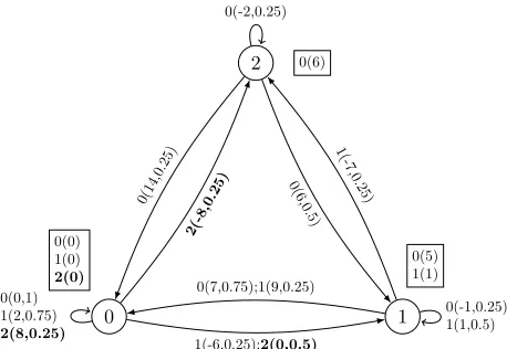
0.25,P(Dt = 1) = 0.5,P(Dt = 2) = 0.25respectively. The initial distribution µ(0) = 1. In this infinite-horizon MDP, the reward function is deterministic and transition-based. The simplified reward functionr0 can be calculated by Equation (2), which is state-based. As illustrated in Fig-ure 1, now we have two MDPs with different reward func-tions:hS, A, r, p, µ, γiandhS, A, r0, p, µ, γi.
Reward Distribution Estimation
Since we consider risk from the distributional perspec-tive instead of the expected return, we need to estimate the reward distribution. The functional distribution estima-tions in Makrov reward processes have been studied for decades (Woodroofe 1992; Meyn and Tweedie 2009). How-ever, there is no related central limit theorem for the dis-counted sum of rewards (return). To simplify the estimation, we estimate the return distribution by considering mean and variance only, which implies the assumption that the return is approximately normal. For an infinite-horizon Markov re-ward process with a deterministic state-based rere-ward func-tion, Sobel (1982) presented the return variance formula for Markov reward processes.
Theorem 3. (Sobel 1982) Given an infinite-horizon Markov reward processhS, r0π, pπ, γiwith the finite state spaceS= {1,· · ·,|S|}, the reward function rπ0 deterministic state-based and bounded, and the discount factor γ ∈ (0,1). Denote the transition matrix by P, in which P(x, y) =
0 1
2
0(14,0.25)
2(-8,0.25)
0(6,0.5) 1(-7,0.25)
1(-6,0.25);2(0,0.5)
0(7,0.75);1(9,0.25) 0(-2,0.25)
0(0,1) 1(2,0.75)
2(8,0.25)
0(-1,0.25) 1(1,0.5) 0(0)
1(0)
2(0)
0(5) 1(1) 0(6)
Figure 1: An MDP with a transition-based reward func-tion and its counterpart with a state-based reward funcfunc-tion following reward simplication. Labels along transitions de-note a(r(x, a, y), p(y|x, a)), and labels next to states de-note a(r0(x, a)), the state-based reward function simpli-fied with Equation (2). For example, the labels in bold are interpreted as follows: the label2(0,0.5)below the transi-tion from 0 to 1 means that the reward r(0,2,1) = 0and the transition probability is 0.5; the label 2(0) near state 0 means whenXt = 0andKt = 2, the simplified reward
r0(0,2) = 0.
pπ(y | x), x, y ∈ S. Denote the conditional return
expec-tation byvx = E(Φ | X0 = x)for any deterministic ini-tial state x ∈ S, and the conditional expectation vector by v. Similarly, denote the conditional return variance by
ψx = V(Φ | X0 = x), and the conditional variance vec-tor byψ. Let θdenote the vector whose xth component is
θx=Py∈Spπ(x, y)(r0π(x) +γvy)2−v2x. Then
v=r0+γP v= (I−γP)−1r0,
ψ=θ+γ2P ψ= (I−γ2P)−1θ.
Now with the aid of Theorem 3, we can estimate the re-turn distribution for the ergodic Markov reward process. No-tice that the variance formula is for Markov reward process with a deterministic reward function only. In next section, we generalize the transformation for the Markov reward pro-cesses and MDPs in different cases, estimate the return dis-tribution in the inventory control problem with the aid of a transformation, and compare it with the one from the reward simplification.
State-Augmentation Transformations
In this section, we propose the state-augmentation transfor-mations (SATs) for three cases.• Case 1: a Markov reward process with a stochastic, transition-based reward function;
• Case 3: an MDP with a randomized policy space.
Case 1 can be considered as an MDP with a rST (or
rSS) and a deterministic policy. Case 2 refers to the con-strained MDPs. Case 3 describes a direct policy search (gra-dient descent method, for example) scenario from a risk-sensitive perspective. In all the three cases, the reward func-tions are often simplified in a similar way as in Equation (2), which will lose all moment information except for the first one (mean). Noticing that the state-transition transforma-tion (Ma and Yu 2017) is for a Markov reward process with a deterministic, transition-based reward function, which we define as Case 0. Since Case 0 is a special case of Case 1, we denote this relationship byCase 0≺Case 1. Similarly, the four cases have the relationship
Case 0≺Case 1≺Case 2≺Case 3.
Concisely, we review the original state-transition transfor-mation in Algorithm 1, give a theorem (Theorem 4) and its proof for the most general Case 3, and two corollaries (Corollary 5, Corollary 6) for Case 2 and 1. Considering the relationship between the cases, all needed algorithms and theorems for different cases can be derived from the con-structive proof for Theorem 4 with some slight changes.
SAT for Case 3
We give the transformation theorem for MDPs with arST (Equation (1)) in a control setting and prove it as follows.
Theorem 4 (Transformation for MDPs). Given an MDP
hS, A, r, p, µiwithrstochastic and transition-based, there exists an MDPhS†, A, r†, p†, µ†iwithr†deterministic and state-based, such that for any given policy (possibly ran-domized) for hS, A, r, p, µi, there exists a corresponding policy forhS†, A, r†, p†, µ†i, such that both Markov reward processes share the same return distribution.
Proof. The proof has two steps. Step 1 constructs a second MDP and shows that, for every possible sample path in the first MDP, there exists a corresponding sample path in the second MDP. Step 2 proves that, the probability of any pos-sible sample path in first MDP equals to the probability of its counterpart in the second MDP.
Step 1: DefineS ={1,· · ·,|S|}. Forx, y∈S, a∈Ax, define J = supp(r(· | x, a, y)). Define S‡ = S2 ×
A×J. In order to remove the dependency of the initial state distribution on policy, define a null state spaceW =
{w1,· · ·, w|S|}, andW ∩S‡ = ∅. Define the state space
S†=S‡∪W.
For all x† = (x, a, y, j), y† = (y, a0, y0, j0) ∈ S†, wherey0∈S, a0 ∈Ay, j, j0∈J, define the state-based reward functionr†(j|x†,·) = 1, andr†(0|w·,·) = 1;
de-fine the transition kernelp†(y†|x†, a0) =p(y0|y, a0)r(j0 | y, a0, y0), andp†(x† |wx, a) =p(y|x, a)r(j|x, a, y); the initial state distributionµ†(wx) =µ(x).
Now we have two MDPs. LetM DP1 = hS, A, r, p, µi,
and M DP2 = hS†, A, r†, p†, µ†i. For any sample path (x1, a1, j1, x2, a2, j2, x3, a3, j3, x4· · ·) in M DP1, there
exists a sample path
(wx1, a1,0,(x1, a1, j1, x2), a2, j1,(x2, a2, j2, x3), a3,
j2,(x3, a3, j3, x4),· · ·)
inM DP2. Therefore, we proved that for every possible
ple path for the first MDP, there exists a corresponding sam-ple path for the second MDP.
Step 2: Next we prove the probabilities for the two sample paths are equal. Here we prove it by mathematical induction. Set time epoch tonafter the firstxn+1inM DP1, and after
the first(xn, an, jn, xn+1)inM DP2.
Denote the partial sample path till epochibyιiinM DP1.
Given anyπ∈ΠRforM DP1, the probability for the
sam-ple path before epoch1inM DP1is
P(ι1= (x1, a1, j1, x2)) =
µ(x1)π(a1|x1)p(x2|x1, a1)r(j1|x1, a1, x2).
There exists a policy π† for M DP2, withπ†(a | wx) =
π(a|x), andπ†(a|x†) =π(a|y). The probability for the sample path before epoch1inM DP2is
P(ι†1= (wx1, a1,0,(x1, a1, j1, x2)))
=µ(wx1)π†(a1|wx1)p((x1, a1, j1, x2)|wx1, a1) =P(ι1= (x1, a1, j1, x2)).
Therefore, at epoch1, the two partial sample paths share the same probability.
Assuming that the two partial sample paths share the same probability at epochn, then the probability for the sample path before epochn+ 1inM DP1is
P(ιn+1= (ιn, xn+1, an+1, jn+1, xn+2))
=P(ιn= (x1,· · ·, xn, an, jn, xn+1))π(an+1|xn+1)×
p(xn+2|xn+1, an+1)r(jn+1|xn+1, an+1, xn+2).
The probability for the sample path before epochn+ 1in
M DP2is
P(ι†n+1= (ι†n, an+1, jn,(xn+1, an+1, jn+1, xn+2))) =
P(ι†n= (wx1,· · · ,(xn, an, jn, xn+1)))×
π†(an+1|(xn, an, jn, xn+1))×
p((xn+1, an+1, jn+1, xn+2)|(xn, an, jn, xn+1), an+1)×
r(jn |(xn, an, jn, xn+1), an+1)
=P(ιn+1 = (ιn, xn+1, an+1, jn+1, xn+2)).
By induction we proved that, the probability of any pos-sible sample path inhS, A, r, p, µiequals to the probability of its counterpart in hS†, A, r†, p†, µ†i. As a subsequence of a sample path, the reward sequence {Rt} is preserved with a null reward at t = 1. Given the discount factor γ, we can compensate this time drift effect simply by setting
r†(x†) =r†(x†)/γto preserve the return distribution.
The-orem 4 is proved.
0 1 2
14(0.25)
-8(0.25)
6(0.5) -7(0.25)
0(0.5)
9(0.25) -2(0.25)
8(0.25) 1(0.5)
0 1
6
(a)
0–0 0–1 0–2
1–0 1–1 1–2
2–0 2–1 2–2
0.25
0.5
0.25
0.25 0.5
0.25
0.25 0.25
0.25 0.5 0.25
8 0 8
9 1 -7
14 6 -2
(b)
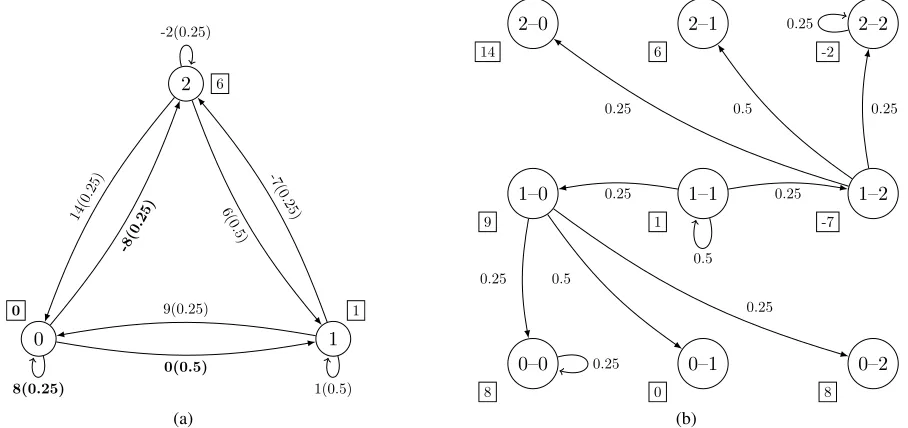
Figure 2: (a) The Markov reward process for the MDP in Figure 1 with the policyπ. This Markov process has a transition-based reward function. The labels along transitions denoterπ(x, y)(pπ(x, y)), and the labels r0π(x) near states denote the state-based reward function simplified with Equation (2); (b) The transformed Markov reward process with a state-based reward function. For a Markov reward process with a deterministic transition-based reward function, the transformation takes transitions as states and attach each possible reward to a state, in order to preserve the reward sequence. The labels along transitions denote
p†π(x†, y†), and the labels r†(x†) near states denote the state-based reward function from the transformation.
measures (Ruszczy´nski 2010), since{Rt}can be preserved as well. It should also be pointed out that, since the state space is augmented, the SATs has an effect on the compu-tational complexity. Denote the complexity for an algorithm byT(|S|,|A|), it becomesT(|S2×A×J|+|S|,|A|)when
the SAT for Case 3 is implemented.
SAT for Case 2 and 1
Here, we present SATs for MDPs in policy evalua-tion settings. Given an MDP with a randomized pol-icy π ∈ ΠR, the reward function is often simplified as well. Taking a deterministic state-based reward func-tionrDS for example, the reward function is simplified to
P
y∈Sπ(a|x)rDS(x, a), x, y ∈S, a ∈Ax. In order to pre-serve the reward sequence, one way is to consider action in a “situation” in Remark 1.
Remark 1 (State augmentation in the transformations). In order to transform a Markov reward process with arST (or
rSS,rDT) to the one with arDS, and preserve the return se-quence at the same time, a bijective mapping between a new “augmented” state space and the possible “situation” space is needed. For a Markov reward process with rST, a pos-sible situation can be defined by a tuplehx, y, ji, in which
x, y∈S, j∈supp(rST(· |x, y)).
Next, we present the following corollaries for Case 2 and Case 1.
Corollary 5 (Transformation for MDP with a random-ized policy). For a Markov decision processhS, A, r, p, µi
with r stochastic and transition-based, and a randomized policy π ∈ ΠR, there exists a Markov reward process hS†, r†π, p†π, µ†πiwithr†πdeterministic and state-based, such that both processes share the same return sequence.
Similarly, we present a corollary for Case 1, which is a special case of Corollary 5.
Corollary 6 (Transformation for Markov process with a stochastic transition-based reward function). For a Markov reward process hS, rπ, pπ, µπi with rπ stochastic and
transition-based, there exists a Markov reward process
hS†, r†π, p†π, µ†πiwithr†πdeterministic and state-based, such
that both processes share the same return sequence.
SAT for Case 0
When we use Q-learning, or other Q-function (value tion) based learning methods in an MDP with a reward func-tion which is not deterministic and state-based, it implies a reward simplification similar to Equation (2). This sim-plification changes the reward distribution as well as a risk measure. In this subsection, we show the effect on the dis-tribution from the reward simplification. We apply the state-transition transformation (Ma and Yu 2017)—which is the SAT for Case 0—in an infinite-horizon with a discount fac-tor setting, estimate the reward distribution and the VaR re-sult, and compare them with the ones from reward simplifi-cation.
func-Algorithm 1State-Transition Transformation (for Case 0) Input:Markov reward processhS, rπ, pπ, µi.
Output:Markov reward processhS†, r†π, p†π, µ†i. Generate the state spaceS†=S×S;
for allx† = (x, y)wherex, y∈Sdo
Construct the reward functionr†π(x†) =rπ(x, y); Construct the transition kernel
p†π(x† |y†) =pπ(y | x)for ally† = (·, x)∈S†, and
p†π(x†|y†) = 0otherwise; Set the initial state distribution
µ†(x†) =µ(x)pπ(y|x); end for
tion following reward simplication. In this MDP, consider a deterministic policyπ = [2,1,0]—to order 2, 1, 0 item(s) when the inventory level is 0, 1, 2, respectively—then we have a Markov reward process illustrated in Figure 2(a). In order to attach each possible reward value to a state to con-struct arDS, we consider each transition as a state, and ap-ply theState-Transition Transformation (Algorithm 1 (Ma and Yu 2017)). The transformed Markov reward process is presented in Figure 2(b), where only some of the transitions are shown. Given the same Markov reward process without the transformation, the reward function is often simplified by Equation (2), which only preserves the expectation.
20 30 40 50 60 70 80 90 Return
0.0 0.2 0.4 0.6 0.8 1.0
Percentage
Ave. emp. return dist. with error bar Est. return dist. with transformation Est. return dist. with reward simplification
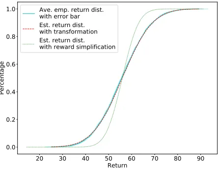
Figure 3: Comparison among the averaged empirical return distribution with error region, the estimated return distribu-tion from the transformadistribu-tion, and the estimated return distri-bution from the reward simplification.
Now we set γ = 0.95 and compare the two return distributions—one from the transformation and the other from the reward simplification—with the averaged empirical return distribution. Since there is no central limit theorem for discounted Markov processes, to simplify the estima-tion, we estimate the return distribution by involving mean and variance only, which implies the assumption that the
re-turn is approximately normal. With the aids of Theorem 3, the two distributions are shown in Figure 3. The averaged empirical return distribution is from a simulation repeated 50 times with a time horizon 1000, with the error region representing the standard deviations of the means along re-turn axis. The Kolmogorov–Smirnov statisticDKS (Durbin 1973) is used to quantify the distribution difference (er-ror). Denote the averaged empirical return distribution by
ˆ
FΦπ, the estimated distribution for the transformed process byQπ
Φ, and the estimated distribution for the process with
the reward simplification byQ0π
Φ. For the case in Figure 3,
DKS(Q0Φπ,FˆΦπ) = supφ∈R|Q
0π
Φ(φ)−FˆΦπ(φ)| ≈ 0.145,
and DKS(QπΦ,Fˆ
π
Φ) ≈ 0.012. The results show that, the
reward simplification leads to a nontrivial estimation error (0.145 > 0.012). Notice that the direct use of Q-learning will result in a risk measure on a learned distribution, which is supposed to converge to the estimated distribution with the reward simplification.
20 30 40 50 60 70 80 90 Return
0.0 0.2 0.4 0.6 0.8 1.0
Percentage
Ave. emp. VaR function Est. VaR function with normal dist. assumption Est. VaR function with reward simplification
Figure 4: Comparison among the averaged empirical VaR function, the estimated VaR function from the transforma-tion, and the estimated VaR function from the reward sim-plification.
Now consider the VaR objective (VaR Definition 2 for ex-ample). The VaR function is obtained by enumerating the deterministic policies. Figure 4 shows the two estimated VaR functions. Since the VaR function can also be regarded as a return distribution, we can still use DKS to measure the error from the reward simplification, and in this case
DKS ≈ 0.150. Denote the optimal quantile for the MDP with the reward simplification by ηˆτ, then the error bound for the optimal quantilesup{|ηˆτ−ητ| :τ ∈R} ≈0.150,
which is nontrivial in this risk-sensitive problem.
Remark 2 (Smaller variance from reward simplification).
transition-based reward function for example. Considering the possible rewards for the same current state as a group, the variance forRtincludes the variances between groups and the vari-ances within groups. When the reward function is simplified with Equation (2), the variances within groups are removed, so the variance is smaller.
From the inventory example we can see that, some meth-ods require Markov processes to be with deterministic and state-based reward functions only, and the reward simplifi-cation changes the reward sequences (distributions). If we want to use Q-learning, or other methods for Markov pro-cesses withrDS in a risk-sensitive scenario, we should im-plement an appropriate SAT first.
Related Works
The risk concerns arise in RL in two aspects. One refers to the “external” uncertainty in the model parameters, and this problem is known as robust MDPs. In the robust MDPs people optimize the expected return with the worst-case pa-rameters, which belongs to a set of plausible MDP param-eters. For example, an MDP with uncertain transition ma-trices (Nilim and Ghaoui 2005). The other one refers to the “internal” risk, which studies the stochastic property of the process. In general, there are three internal risk-sensitive objective classes in RL area, which have been studied for decades. One is the mean-variance risk measure (White 1988; Sobel 1994; Mannor and Tsitsiklis 2011), also known as the modern portfolio theory, in which the expected re-turn is maximized with a given risk level (variance). The other is target-percentile risk measure (Filar et al. 1995; Wu and Lin 1999). This risk measure formulate the objec-tive in terms of the probabilities of certain targets (or quan-tiles), and optimize, for example, the expected return. An-other is utility risk measure, in which the exponential util-ity function is concerned. The internal risk concerns arise not only mathematically but also psychologically. A clas-sic example in psychology is the “St. Petersburg Paradox,” which refers to a lottery with an infinite expected reward, but people only prefer to pay a small amount to play. This problem is thoroughly studied in utility theory, and a recent study brought this idea to RL (Prashanth et al. 2016). Some risk measures are coherent (Artzner et al. 1998), which share some intuitively reasonable properties (convexity, for exam-ple). Ruszczy´nski and Shapiro (2006) presented a thorough study on coherent risk optimization.
Q-learning has been studied in risk-sensitive RL for decades. Many risk-sensitive Q-learning studies are for MDPs with anrDS. Borkar (2002) proved the convergence of Q-learning for an exponential utility cost objective with an ordinary differential equation method. A trajectory-based algorithm which combines policy gradient and actor-critic methods was presented to solve a CVaR-constrained prob-lem (Chow et al. 2017). For robust MDP probprob-lems, with con-sidering a set of general uncertainties (random action, un-known cost and safety hazards), an approach was provided to compute safe and optimal strategies iteratively (Junges et al. 2016). Q-learning has also been used to provide risk-sensitive analysis on the fMRI signals, which provides a
bet-ter inbet-terpretation of the human behavior in a sequential de-cision task (Shen et al. 2014). The expectation-based worst case risk measure might not need the proposed SATs. For example, the minimax risk measures studied in (Huang and Haskell 2017). For a comprehensive survey on safe RL, see (Garc´ıa and Fern´andez 2015).
Conclusion
The proposed SATs transform MDPs and Markov reward processes with stochastic transition-based reward tions into ones with deterministic state-based reward func-tions, and preserve the reward sequences (and distributions) for risk-sensitive objectives. In an infinite-horizon time-homogeneous MDP for an inventory control problem, we illustrate the error on the distribution from the reward sim-plification. Taking the advantage of the variance formula presented by Sobel (1982), we estimate the return distribu-tion for a Markov reward process. Since many RL methods require the reward function to be deterministic and state-based, the transformation is needed for the MDPs with other types of reward functions in the risk-sensitive problems. We generalize the transformation (Ma and Yu 2017) in different settings, and consider VaR as an example to show the effect of reward simplification on distribution.
In many practical problems, the rewards are simplified to deterministic and state-based. When the MDP is with a re-ward function which is not anrDStype, the direct use of Q-learning also implies such a reward simplification. In this pa-per, the error from the reward simplification on distribution is illustrated, which is crucial in risk-sensitive cases. By im-plementing the transformation instead of the reward simpli-fication, the MDPs with different types of reward functions and (or) randomized policies are transformed to the ones with deterministic and state-based reward functions with an intact reward distribution.
The essence of the SATs is to attach each possible reward value to an augmented state to preserve the reward sequence. This attachment is crucial in risk-sensitive reinforcement learning, considering the wide application of value function and function. Without the proposed SATs, the learned Q-function (value Q-function) only estimates the expected value of a given state-action pair (state) when the reward function is (stochastic) transition-based. Now with the SATs, the Q-function (value Q-function) can be considered as an approxi-mation of the “real” value of a given augmented state-action pair (state). In other words, the proposed transformations “transform” the uncertainties from the transition, action, and the stochasticity of the reward function to the augmented state space. The proposed SATs present a platform for Q-learning in risk-sensitive RL, and we believe that many re-lated studies should be revisited with the proposed SATs instead of applying the common-used reward simplification directly.
Acknowledgments
and Engineering Research Council of Canada (NSERC) un-der Grants 509935 and 512046.
References
Altman, E. 1999.Constrained Markov Decision Processes. CRC Press.
Artzner, P.; Delbaen, F.; Eber, J.; and Heath, D. 1998. Co-herent measures of risk.Mathematical Finance9(3):1–24. Berkenkamp, F.; Turchetta, M.; Schoellig, A.; and Krause, A. 2017. Safe model-based reinforcement learning with stability guarantees. InProceedings of the 31st Advances in Neural Information Processing Systems (NIPS), 908–918. Borkar, V. S. 2002. Q-learning for risk-sensitive control.
Mathematics of Operations Research27(2):294–311. Chow, Y.; Ghavamzadeh, M.; Janson, L.; and Pavone, M. 2017. Risk-constrained reinforcement learning with per-centile risk criteria. The Journal of Machine Learning Re-search18(1):6070–6120.
Durbin, J. 1973. Distribution Theory for Tests based on the Sample Distribution Function. SIAM.
Filar, J. A.; Krass, D.; Ross, K. W.; and Member, S. 1995. Percentile performance criteria for limiting average Markov decision processes. IEEE Transactions on Automatic Con-trol40(I):2–10.
Garc´ıa, J., and Fern´andez, F. 2015. A comprehensive survey on safe reinforcement learning. Journal of Machine Learn-ing Research16(1):1437–1480.
Gilbert, H., and Weng, P. 2016. Quantile reinforcement learning.arXiv:1611.00862.
Huang, W., and Haskell, W. B. 2017. Risk-aware Q-learning for Markov decision processes. InProceedings of the 56th IEEE Conference on Decision and Control (CDC), 4928– 4933.
Junges, S.; Jansen, N.; Dehnert, C.; Topcu, U.; and Katoen, J.-P. 2016. Safety-constrained reinforcement learning for MDPs. InProceedings of the 22nd International Conference on Tools and Algorithms for the Construction and Analysis of Systems (TACAS), 130–146. Springer.
Kusuoka, S. 2001. On law invariant coherent risk measures. InAdvances in Mathematical Economics. Springer. 83–95. Ma, S., and Yu, J. Y. 2017. Transition-based versus state-based reward functions for MDPs with Value-at-Risk. In
Proceedings of the 55th Annual Allerton Conference on Communication, Control, and Computing (Allerton), 974– 981.
Mannor, S., and Tsitsiklis, J. 2011. Mean-variance op-timization in Markov decision processes. In Proceedings of the 28th International Conference on Machine Learning (ICML), 1–22.
Meyn, S. P., and Tweedie, R. L. 2009. Markov Chains and Stochastic Stability. Springer Science & Business Media. Nilim, A., and Ghaoui, L. E. 2005. Robust control of Markov decision processes with uncertain transition matri-ces.Operations Research53(5):780–798.
Prashanth, L. A.; Jie, C.; Fu, M.; Marcus, S.; and Szepesv´ari, C. 2016. Cumulative prospect theory meets reinforce-ment learning: Prediction and control. In Proceedings of the 33rd International Conference on Machine Learning (ICML), 1406–1415.
Puterman, M. L. 1994. Markov Decision Processes: Dis-crete Stochastic Dynamic Programming. Wiley.
Riedel, F. 2004. Dynamic coherent risk measures. Stochas-tic Processes and their Applications112(2):185–200. Ruszczy´nski, A., and Shapiro, A. 2006. Optimization of convex risk functions.Mathematics of Operations Research
31(3):433–452.
Ruszczy´nski, A. 2010. Risk-averse dynamic programming for Markov decision processes.Mathematical Programming
125(2):235–261.
Scheff´e, H. 1999. The Analysis of Variance. John Wiley & Sons.
Shen, Y.; Tobia, M. J.; Sommer, T.; and Obermayer, K. 2014. Risk-sensitive reinforcement learning. Neural Computation
26(7):1298–1328.
Sobel, M. J. 1982. The variance of discounted Markov de-cision processes. Journal of Applied Probability19(4):794– 802.
Sobel, M. J. 1994. Mean-variance tradeoffs in an undis-counted MDP. Operations Research42(1):175–183. White, D. J. 1988. Mean , variance , and probabilistic crite-ria in finite Markov decision processes : A review. Journal of Optimization Theory and Applications56(1):1–29. Woodroofe, M. 1992. A central limit theorem for functions of a Markov chain with applications to shifts. Stochastic processes and their Applications41(1):33–44.
Wu, C., and Lin, Y. 1999. Minimizing risk models in Markov decision process with policies depending on target values. Journal of Mathematical Analysis and Applications