Congestion Graphs for Automated Time Predictions

(1)

The Thirty-Third AAAI Conference on Artificial Intelligence (AAAI-19)

Congestion Graphs for Automated Time Predictions

Arik Senderovich, J. Christopher Beck

Mechanical and Industrial Engineering University of Toronto

Canada [email protected]

[email protected]

Avigdor Gal

Industrial Engineering and Management Technion-Israel Institute of Technology

Israel [email protected]

Matthias Weidlich

Dept. of Computer Science Humboldt University zu Berlin

Germany

[email protected]

Abstract

Time prediction is an essential component of decision making in various Artificial Intelligence application areas, including transportation systems, healthcare, and manufacturing. Predic-tions are required for efficient resource allocation and schedul-ing, optimized routschedul-ing, and temporal action planning. In this work, we focus on time prediction incongestedsystems, where entities share scarce resources. To achieve accurate and ex-plainable time prediction in this setting, features describing system congestion (e.g., workload and resource availability), must be considered. These features are typically gathered using process knowledge, (i.e., insights on the interplay of a system’s entities). Such knowledge is expensive to gather and may be completely unavailable. In order to automatically extract such features from data without prior process knowl-edge, we propose the model ofcongestion graphs, which are grounded in queueing theory. We show how congestion graphs are mined from raw event data using queueing theory based assumptions on the information contained in these logs. We evaluate our approach on two real-world datasets from health-care systems where scarce resources prevail: an emergency department and an outpatient cancer clinic. Our experimental results show that using automatic generation of congestion features, we get an up to23%improvement in terms of rela-tive error in time prediction, compared to common baseline methods. We also detail how congestion graphs can be used to explain delays in the system.

Introduction

Accurate time prediction is important in domains where hav-ing an accurate estimate of resource availability and the du-ration of tasks is critical for planning, scheduling, resource allocation, and coordination. In healthcare, the time until a patient sees a provider in an emergency department is cru-cial for ambulance routing and provider scheduling (Ang et al. 2015). Similarly, in smart cities, predicted travel and arrival times of public transportation feed directly into rout-ing and dispatchrout-ing (Botea, Nikolova, and Berlrout-ingerio 2013;

Wilkie et al. 2011). In manufacturing, in turn, predictions of cycle times for a product are used to set customer due dates and anticipate job completion times (Backus et al. 2006).

An effective approach to solve a time prediction prob-lem is to formulate it as a supervised learning task, where future time points are predicted based on raw event data (Senderovich et al. 2015). This data is commonly avail-able in the form ofevent logs, recordings of the behavior of a system, which contain temporal information. For example, every visit to the emergency department is associated with a sequence of timestamped events that the patient experienced (e.g., start of triage and end of treatment).

Previous work has shown that congestion has a substan-tial impact on the total time spent in a system (Gal et al. 2017) and hence on the quality of time prediction. However, event logs lack explicit information on the load imposed by arriving entities that are processed by shared (and scarce) resources. State-of-the-art methods, therefore, consider ad-ditional features that capture congestion of shared resources. These features are elicited by gathering extensive knowl-edge about the underlying process (e.g., by conducting inter-views with stakeholders) and subsequently computed from the event logs (Ang et al. 2015). However, process knowl-edge is expensive to gather and not always easy to elicit as stakeholders often lack a global view of the process. It is well-known that elicitation of process knowledge is hindered by its fragmentation across stakeholders, their focus on individual entities, and a general lack of conceptualization capabili-ties (Rosemann 2006; Frederiks and van der Weide 2006; Dumas et al. 2018). In addition, manual feature elicitation is often time consuming and prone to biases and errors. The process of feature generation is considered an art, making it difficult to automate (Khurana, Samulowitz, and Turaga 2018).

In this work, we address the challenge ofautomatically

(2)

that analyzes the impact of congestion on a system’s perfor-mance (Bolch et al. 2006). Our contribution is threefold. 1. We introducecongestion graphs, dynamic networks that

capture queueing information.

2. We present a declarative mining procedure that automati-cally constructs congestion graphs from event data without the need for process knowledge.

3. We show how to extract congestion-related features from congestion graphs.

We empirically test our approach using event logs from two real-world healthcare systems, predicting the time to meet the first physician in an emergency department and the total time spent in an outpatient cancer clinic. Incorporating our congestion features improves the relative error of prediction by up to23%and14%, respectively, compared to baseline prediction methods using the same process knowledge.

Data-Driven Time Predictions

In this section, we define our data model in the form of event logs and then pose the problem of automated time prediction via supervised learning. We conclude the section with an overview of our approach to generate congestion-related features from an event log in order to solve the time prediction problem.

Event Logs

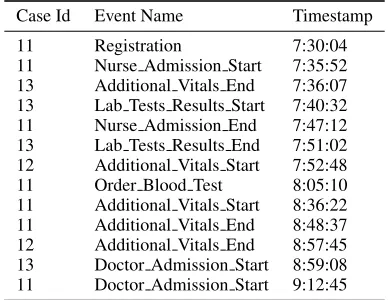
As our data model, we consider event data as collected by modern information systems (i.e.,event logs) that trace the events that occur in the underlying system (van der Aalst 2016). For example, in a hospital setting, an event log will comprise patient pathways, represented by a sequence of timestamped services that denote treatment steps (e.g., XRAY ordering, start of physical examination,etc.). 1 is a sample from the event log of an emergency department. Here, the handling of a specific entity (i.e., a patient) is represented by the notion of acasethat is encoded by a case identifier present in all log entries. Event logs represent raw data for individual cases, but do not contain explicit system-level information (e.g., the number of available resources and the number of cases waiting for a service).

Table 1: An event log of an emergency department.

Case Id Event Name Timestamp

11 Registration 7:30:04

11 Nurse Admission Start 7:35:52 13 Additional Vitals End 7:36:07 13 Lab Tests Results Start 7:40:32 11 Nurse Admission End 7:47:12 13 Lab Tests Results End 7:51:02 12 Additional Vitals Start 7:52:48 11 Order Blood Test 8:05:10 11 Additional Vitals Start 8:36:22 11 Additional Vitals End 8:48:37 12 Additional Vitals End 8:57:45 13 Doctor Admission Start 8:59:08 11 Doctor Admission Start 9:12:45

To formalize the notions of cases and their traces in event

logs, letI,E, andT be the finite universes of case identifiers, event names, and timestamps, respectively. Then, anevent log L ⊆ (I × E × T)is a set oflog entries, triplets that combine a case, an event name, and a timestamp.

We define some short-hand notation to refer to the log entries of a single case. Given a logL, thetraceσiof case

i∈ Icomprises all the related log entries in order:

σi=h(i, ei1, ti1),(i, e2i, ti2), . . . ,(i, ein, tin)i withσi_{(q) = (i, e}i

q, tiq) ∈ L,1 ≤ q ≤ n, such thattq <

tr for1 ≤ q < r ≤ n(log entries are ordered by their timestamp) andS

1≤q≤n{(i, e i

q, tiq)} = {(ir, er, tr) ∈ L |

ir=i}(the trace contains all log entries of casei). As such,

ei_qandti_qdenote the event name and timestamp of theq-th log entry of the trace of casei, respectively. We assume that the first eventei1is an arrival event of caseiinto the system. In

what follows, we shall omit sub- and superscripts whenever clear from the context. Moreover, we write |σi_| ₌ _n

i to denote the length of thei-th trace.

Time Prediction with Supervised Learning

We are interested in predicting the timestamp of an event related to a specific case. For example, in an emergency department, we are interested in the time that a patient sees a physician for the first time, as it is crucial information for online ambulance routing (for acute patients) and for a patient’s choice of an emergency department (for low-acuity patients) (Ang et al. 2015). In other contexts, such as the treatment of cancer patients, the time until the end of the last treatment step is an important indicator for quality-of-service. Theprediction targetis therefore the timete, when a pa-tient first reaches a specific evente ∈ E, conditioned on timet1of arrival (e1). Using supervised learning, every log

entry in the training set is given a labely =te−t1for the

prediction target, denoting the universe of such labels byY. Consequently, the input for the learning algorithm is a labeled event log denoted byLy ⊆ L × Y. We aim to obtain a func-tionh: L → Y, which maps log entries to corresponding labels (Shalev-Shwartz and Ben-David 2014).

A main challenge when applying supervised learning to solve prediction problems is to obtain features that explain the target variable. However, in systems with shared and scarce resources, raw event recordings do not contain congestion related information, such as system load and the number of available resources. In this work, we therefore propose a feature transformation functionφ : L × Y → X × Ythat maps raw labeled event recordings into a set of features (X) with the following two capabilities:

(i) The proposed method is automatically applicable with-out prior knowledge of the system under investigation or the specific semantics of events recorded in the log; (ii) The proposed method is grounded in well-established results from queueing theory, thereby guiding the fea-ture generation procedure with insights on the impact of congestion on the system’s temporal behavior.

Approach Overview

(3)

EHR Event Log

Mining Congestion Graphs

Congestion Graphs

Infinite Resources

Steady-State

State-Aware

Feature Learning _Enriched

Data

Congestion Graphs

Infinite Resources

Steady-State

State-Aware

Mining Congestion Graphs

Feature Learning EHR Event Log

Enriched Data

Mining Congestion

Graphs EHR

Event Log

Enriched Data Feature

Learning Congestion

Graphs

Infinite Resources

Steady-State

State-Aware

Congestion Graph Discovery

Event Log Enriched

Event Log Feature

Extraction Congestion

Graphs

Infinite Resources

Snapshot

Markovian

Congestion Graph Mining

Event Log Enriched

Event Log Feature

Extraction Congestion

Graph

Figure 1: Our solution to generate congestion features.

log, we first mine congestion graphs, graphical representa-tions of the dynamics observed in the system. These dynamic graphs represent the flow of entities in terms of events and are labeled with performance information that is extracted from the event log. Extraction of such performance information is grounded in some general assumptions on the system dynam-ics: in this work, on a state representation of an underlying queueing system. Lastly, we create a transformation function

φGthat encodes the labels of a congestion graph into respec-tive features. This feature creation yields an enriched event log, which can be used as input for a supervised learning method.

Congestion Graphs

We start the section with an overview of a general queueing model that serves as our theoretical basis, before introduc-ing the model of congestion graphs. Then, we demonstrate mining of congestion graphs and show how these graphs are used for feature extraction.

Generalized Jackson Networks

For time prediction in queueing networks, we consider the model of a Generalized Jackson Network (GJN), the most general model in single-server queueing theory (Gamarnik and Zeevi 2006). A GJN describes a network of queueing stations, where entities wait for a particular service (e.g., a treatment step) that is conducted by or uses shared resources. The entities are assumed to be non-distinguishable and may arrive exogenously into any of the queueing stations ac-cording to a renewal process. Upon arrival, entities are served in a First-Come First-Served order by a single resource, with service times being independent and identically distributed. Hence, the length-of-stay (or sojourn time) at a queueing station is the sum of waiting time and service time. When entities complete service at a station, they are either routed to the next station or depart the system. Routing is assumed to be Bernoulli distributed: a coin is flipped at the end of service to decide on the next station (or departure).

As a GJN model postulates that each station has a single resource, multiple resources are modeled by an increased processing rate of a station: the service rate is multiplied by the number of resources.

The state of the GJN corresponds to a Markov process, known as theMarkov state representation(MSR), that com-prises three components: the queue length, the elapsed time since the most recent arrival, and the time since the start of the most recent service (Gamarnik and Zeevi 2006; Chen and Yao 2013). To capture the state at timet, the three components must be measured just prior to timet.

The Model of Congestion Graphs

A congestion graph is a fully-connected, vertex-labeled, di-rected graph,G= (V, F, ω)withV being the vertices and

F = V ×V being the edges. The labeling is based on a universeΩof vertex labels and is time-varying. WithT as the universe of timestamps (as introduced above for event logs), functionω:V × T →Ωassigns a label to vertices at particular points in time. We denoteωt(v)the label of vertex

v∈V at timet∈ T.

In our work, we define congestion graph labels using the MSR of a GJN. Specifically, a congestion graph can be thought of as a GJN where each edge represents a queueing station. The time that cases spend on edges of the congestion graph represent service times, while events (in the event log) correspond to congestion graph vertices. Hence, given a point in timetand an edge(v, v0)of the congestion graph, its MSR is given by a triplet that consists of: (1) the number of cases traveling on edge(v, v0); (2) the time elapsed since the most recent arrival of a case into edge(v, v0); and (3) the time elapsed since the start of the most recent service at(v, v0). However, we cannot determine the edge of an ongoing case at timetas this information is not directly accessible in event logs. At a time pointt, we only know the last event observed for each case (v), without knowing the next event (v0). Thus, we label the vertices of the congestion graph rather than its edges.

Following this idea, we construct the congestion graph

G= (V, F, ω)by setting the verticesV to be the set of all events observed in the log and by assigning time-dependent vertex labels, asapproximationsof the MSR. Specifically, we setωt(v)to be a tuple(n(v, t), (v, t), τ(v, t)), wheren(v, t) is the number of cases for whichvis the most recent event (i.e., the number of cases that are in transition to the service afterv);(v, t)is the total time since these cases visitedv

(i.e., the accumulated partial transition delays); andτ(v, t)

is the time between the two most recent occurrences of the respective eventv.

Feature Extraction from Mined Congestion Graphs

We conclude this section by providing the declarative proce-dure to derive the approximated MSR from an event logL

and demonstrating how to extract features from the mined congestion graph.

Given an event logL, mining of a congestion graph in-volves the extraction of events that yield the vertices of the graph, V = {e ∈ E | (i, e, t) ∈ L}, the identification of dependencies between the events that yield the edges,

F ={(ei

q, eiq+1)∈(E × E)|i∈ I,1≤q <|σi|}, and the definition of the labeling function. As explained above, these labels are defined for particular points in time. However, in practice, the labeling function does not need to be defined for every timestamp inT, but may be limited to the timestamps that appear in the event log (T ={t∈ T |(i, e, t)∈L}).

(4)

1 2

Registration

3 4 5 6

Additional vitals

Lab tests results

Doctor admission

Nurse admission

Order blood test

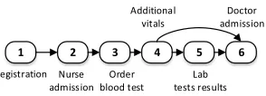
Figure 2: A part of the congestion graph constructed using the event log of 1.

which the last event wasvis given by:

n(v, t) =

i∈ I | ∃1≤q≤ |σi|:eiq=v ∧ t i

q < t < t i

q+1 .

The total elapsed time(v, t)for cases, for which eventvhas just been observed, is calculated as:

(v, t) =

X

i∈I

t−tiq| ∃1≤q≤ |σi|:eiq =v ∧ tiq< t < tiq+1.

Finally, the time between the two most recent occurrences of eventsvprior to timetis defined as:

τ(v, t) =t0−t00, with t0= max

i∈I,1≤q≤|σi_|

ei_q=v∧ti_q<t<ti_q₊₁

ti q

t00= max

i∈I,1≤q≤|σi_|

ei_q=v∧ti_q<t0<ti_q₊₁

ti q

Note that the mining procedure for label derivation has a complexity that is linear in the number of events recorded in the event log: the algorithm makes a single pass over the log to compute the labels.

We illustrate mining a congestion graph using the event log of 1. The general structure of the congestion graph is shown in 2, which maps out all the events and their dependencies as recorded in the event log. Note that for clarity the figure presents only edges that appear Table 1 rather than showing the fully-connected congestion graph. We further illustrate the MSR of one of the graph’s vertices. Consider the fourth event, referring to theadditional vitals. The MSRωt(4)of this event is estimated for time 9:00:00 as follows: Two pa-tients are in transition (papa-tients 11 and 12), their accumulated delay is13m38s, and the delay between the respective treat-ment events is9m8s. Hence, the MSR for the fourth event at time 9:00:00 is given asωt(4) = (2,13m38s,9m8s)).

The vertex labels of the congestion graph induce a set of congestion features. For a graphG= (V, F, ω), the transfor-mation applied to the event log to extract these features at timet, denoted byφG, is simply:

φG:L × Y → L ×Ω× Y,

φG(i, eiq, t i

q, y) = (i, e i q, t

i

q, ωt(eiq)),

withqbeing the most recent event with respect tot.

Evaluation

In this section, we present the main findings of evaluating our congestion mining technique against real-world event logs from two healthcare systems, namely an emergency department and a large outpatient cancer clinic. Our main results are summarized as follows:

• Extracting features from congestion graphs increases the accuracy of time prediction by up to8%with respect to the best benchmark.

• In terms of relative error (i.e., the ratio between the error and the actually observed time), we achieve improvements of up to23%.

• Congestion graphs are able to provide insights into causes of delay via feature ranking.

Experimental Setup and Procedure

We first describe the experimental setup in terms of the two real-world datasets and the benchmarks used to assess the applicability of our approach. We then outline the overall experimental procedure and implementation and define our accuracy evaluation measures.

Datasets and Time Prediction Queries Our experiments use two real-world event logs:

• ED: The event log from the Electronic Health Records of an Israeli emergency department that serves approxi-mately100patients per day. Every patient that enters the emergency department receives a bar-code that is scanned at the start and end of every medical procedure. A subset of the patient treatment events was illustrated in 1 and 2. The actual treatment procedures, however, are more com-plex, as there are 13 different types of treatments. The dataset covers April 2014 to December 2014 and includes approximately42,000patient visits.

• CC:An outpatient cancer clinic (the Dana-Farber Cancer Institute in Boston, MA), in which250health providers serve1,000 patients per day. The dataset is based on a track log that comes from a Real-Time Locating System (RTLS). The resulting event log is based on nearly1,000

RTLS sensors that track patients, physicians, nurses, and equipment with a resolution of3seconds, thereby moni-toring the system in real-time. The recordings contain sen-sor (location) description and the floor number where the tracked entity was observed. The dataset contains record-ings between April 2014 and December 2014.

Comparing the two datasets, we observe that the average length-of-stay for ED is 300 minutes with a standard de-viation of 307 minutes, while for CC patients the stay is approximately 150 minutes with a standard deviation of 120 minutes.EDpatients wait for a physician an average of 60 minutes. Furthermore, the emergency department (ED) oper-ates on a 24/7 basis, while the outpatient clinic (CC) opens at 6:00 and closes for new arrivals at 18:00. Both healthcare systems experience high load during morning hours: forED

the load peaks between 10:00 and noon, while forCC, the high load period spans 9:00 to noon.

(5)

forED, we predict the time-to-physicianupon a patient’s arrival. ForCC, our prediction target is thelength-of-stayof an arriving patient.

Baseline Techniques We compare our approach for time prediction based on features extracted from mined con-gestion graphs against several baseline techniques. First, we consider the long-term average (LongTerm) based on the training set. This technique should perform poorly as it does not account for varying congestion levels. How-ever, it is often used for time prediction in hospitals across the United States (Dong, Yom-Tov, and Yom-Tov 2015; Ang et al. 2015). Second, a refined version of LongTerm is a rolling horizon predictor that is based on the moving average ofH periods (e.g., hours) (Ang et al. 2015). We denote it by Rolling(H) and cross-validate the optimalH

using the training data. Third, we use an hourly average (HourAvg) to accommodate for seasonal effects, deriving time-of-day information from the timestamps assigned to log entries. Fourth, we use thesnapshotpredictor, which predicts time-to-physician and length-of-stay, respectively, based on the wait time of the most recent patient that finished waiting. This result is considered the state of the art in delay prediction for single-station queues (Senderovich et al. 2015).

Experimental Procedure and Implementation We fol-low the training-validation-test paradigm (Friedman, Hastie, and Tibshirani 2001) to evaluate our approach and randomly partition the two datasets into training data and test data. Specifically, for each dataset we make the following four partitions:

• Single month training: We use patients that arrived during April 2014 as training data and patients that were admitted during May 2014 as test data. This reduces the possibility of concept drift, at the expense of reducing the size of the training set.

• Summer months: We use April 2014 - June 2014 for train-ing and test the technique on patients that arrived durtrain-ing July 2014. We leave out winter months as they are known to be heavily loaded (concept drift).

• Entire year: we use April 2014 - October 2014 for training and November 2014 - December 2014 for testing. This increases the variability due to concept drift, yet provides the learning algorithm with much more training data. • Peak hours: We choose the heavily loaded hours for each

of the healthcare systems, as measured by the arrival rates of patients. As in the entire year scenario, we use April 2014 October 2014 for training and November 2014 -December 2014 for testing.

In our experiments, we rely on a state-of-the-art supervised learning algorithm, XGBoost (Chen and Guestrin 2016), im-plemented in Python. It is employed to learn a functionh

(see Motivation) based on the training set, validate its hyper-parameters using cross-validation on the validation set (the training data is partitioned 80/20 chronologically for this purpose), and evaluate prediction accuracy on the test set.

All algorithms for congestion graph mining and feature extraction are implemented in Python and are publicly

avail-able.1Our experiments were conducted on an 8-core server, Intel Xeon CPU E5-2660 v4 @ 2.00GHz, each core being equipped with 32GB main memory, running on Linux Centos 7.3 OS.

Evaluation Measures We measure the accuracy of predic-tion with three empirical measures. First, the Root Mean Squared Error (RMSE) is based on the squared difference between the actual time and the predicted value. Lety_l∗be the actual value ofyl, the time of interest for a log entry of the test setl∈Ltest. Withyˆlbe the predicted value, the RMSE is defined as:

RM SE=

s

1

|Ltest|

X

l∈Ltest

[ ˆyl−yl∗]2.

RMSE quantifies the error in the time units of the original measurements, in our case, seconds (which are converted to minutes below for convenience).

The RMSE is sensitive to outliers (Friedman, Hastie, and Tibshirani 2001). Therefore, in addition, we consider the ab-solute error, which is known to be more robust (Friedman, Hastie, and Tibshirani 2001). Specifically, we use the fol-lowing two measures. The Mean Absolute Error (MAE) is defined as:

M AE = 1

|Ltest|

X

l∈Ltest

|yˆl−yl∗|,

and quantifies the absolute deviation between the predicted value and the real value. The Mean Absolute Relative Error (MARE), in turn, is defined as:

M ARE= 1

|Ltest|

X

l∈Ltest

|yˆl−yl∗|

y∗

l

,

and quantifies the ratio between the absolute error and the pre-dicted value. The latter is used to provide a relative measure for the absolute error, as an error of 10 minutes in a 100-minute length-of-stay is tolerable, while the same error in a 5 minute length-of-stay points toward a significant problem in the method.

Results

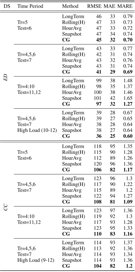
The main results of our experiments are summarized in 2. The rows correspond to all combinations of dataset (ED

andCC), the training period, and the method (‘LongTerm’, ‘Rolling(H)’, ‘HourAvg’, ‘Snapshot’, and ‘CG’ for conges-tion graph). To denote the training and test periods, we use the numeric values of months (e.g., 4 for April). Further, we add the relevant hours for the high load scenario (e.g., 9-12 corresponds to 9:00-noon). The boldfaced values are the dominating methods in terms of the three measures. The values of the first two accuracy measures (RMSE and MAE) correspond to the prediction error in minutes. The third accu-racy measure, namely MARE, is a ratio between the absolute error and the actual time that we wish to predict.

As shown in 2, considering inter-patient dependencies in the data, by means of features extracted from congestion

1

(6)

Table 2: Prediction accuracy based on the test set.

DS Time Period Method RMSE MAE MARE

ED

Tr=5

LongTerm 46 33 0.79 Rolling(H) 47 33 0.73

Test=6 HourAvg 47 33 0.72

Snapshot 47 34 0.74

CG 45 32 0.70

Tr=4,5,6

Snapshot 43 31 0.74

CG 41 29 0.69

Tr=4:10

LongTerm 99 38 1.48 Rolling(H) 98 35 1.37 Test=11,12 HourAvg 100 38 1.46 Snapshot 101 42 1.65

CG 97 32 1.27

Tr=4,5,6

High Load (10-12) Snapshot 38 27 0.64

CG 36 25 0.60

CC

Tr=5

Snapshot 120 96 1.36

CG 106 82 1.17

Tr=4,5,6

Snapshot 122 94 1.27

CG 108 81 1.09

Tr=4:10

LongTerm 123 97 1.36 Rolling(H) 119 92 1.3 Test=11,12 HourAvg 117 93 1.28 Snapshot 123 95 1.33

CG 110 83 1.16

Tr=4,5,6

High Load (9-12) Snapshot 114 93 1.36

CG 104 82 1.2

graphs, improves prediction accuracy beyond the baselines (‘LongTerm’, ‘Rolling(H)’, ‘HourAvg’, ‘Snapshot’), espe-cially when considering the MARE measure. When consider-ing the time-to-physician in the emergency department (ED), congestion features increase prediction accuracy by up to6%. As for relative error (ratio between the error and the actual time), we observe an improvement of23%. This general trend is mirrored for the second dataset. For the cancer clinic (CC), congestion features improve the accuracy of length-of-stay prediction by up to8%, while the relative error is improved by up to14%. The consistent results for both datasets provide evidence that the automatic extraction of congestion features indeed improves the accuracy of time prediction significantly.

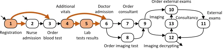
Table 3: Importance of congestion features (EDdataset).

Ranking Feature Description

1 n(1) # of Patients in Reception 2 (5) Elapsed Time: Lab Results 3 (4) Elapsed Time: Additional Vitals

When observing the difference between entire year pre-diction and shorter periods, we encounter a noticeable, yet expected concept drift. Predicting winter months using the beginning of the year is expected to perform worse than short-term predictions, as winter behavior is different due to higher arrival rates into the emergency department and an increased number of cancellations in the outpatient hospital. Specifically, the error grows by a factor of2, compared to summer-time prediction. Testing the different predictors for their robustness to concept drift, we discover that congestion features deteriorate less than other prediction methods across the different selections of time periods for training and test.

Insights using Feature Importance

Providing insights as to the most important features and root-causes for delays in the system is a crucial step when opti-mizing systems. We now take the dataset of the emergency department (ED) as an example to show how the features obtained from congestion graphs provide insights into the root-causes of delays.

We evaluate feature importance by ranking features accord-ing to their role in the prediction task. Specifically, gradient boosting enables the ranking of features in correspondence to their predictive power (Pan et al. 2009). 3 presents the top-3

features given as an output by the cross-validated XGBoost method during heavily loaded hours.

The extracted features (over all times in the event log, hence time index t is omitted) are denoted by

(7)

1 2

Registration

3 4 5 6 7

8 9

10

12

11 13

Nurse admission

Order blood test

Additional vitals

Lab tests results

Doctor admission

Order imaging test Order consultant

Imaging

Imaging decrypting Consultancy Order external exams

External exams

Figure 3: Main treatment events and flows; events and flows of important features are highlighted.

power, as some patients immediately pass from the checking vitals to the physician.

To summarize, an interpretation of feature importance yields insights on root causes of delays in patient treatment. As such, mined congestion graphs provide a means for analy-sis and understanding of the process beyond time prediction.

Related Work

The importance of extracting features that account for con-gestion has been recognized in the literature. A recent work proposes the Q-Lasso method for predicting waiting times in emergency departments (Ang et al. 2015). The authors as-sume full knowledge of the patient flow process and use this knowledge tomanuallydefine queueing features (e.g., the number of patients waiting for a physician) that are inserted into a Lasso regression model for feature selection. Similarly, Senderovich et al. (2015) proposed a single-station queueing model that is heavily based on process knowledge to generate predictive features. In our work, we do not assume a-priori knowledge of the process and the events that we observe in the event log. Furthermore, compared to Senderovich et al. (2015) our approach handles event logs from multi-stage processes.

Liu et al. (2014; 2016) propose a method for discovering a stochastic workflow model from event data that is emitted by a real-time location system. Applied in healthcare, the developed model considers dependencies between patients that stay in the hospital at the same time. However, in these works, the authors assume known relations between sensor locations and activities. This information is used to enrich the data with additional knowledge, while our method does not require a data enrichment step.

Congestion estimation and prediction have been the subject of numerous works in traffic analysis (Liu, Yue, and Krishnan 2013; Van Lint 2008). Most works in this area aim to learn a generative model of dynamic traffic conditions. In contrast, our work is based on discriminative machine learning and formalizes this idea using congestion graphs.

Automated feature generation has been a popular research topic (see Khurana, Samulowitz, and Turaga (2018) and ref-erences within for a review). Specifically, given a pre-defined set of generic feature transformation functions (e.g., sine, squared root, logarithm), a wide range of techniques has been applied to elicit optimal transformation sequences, including reinforcement learning (Khurana, Samulowitz, and Turaga 2018), local search (Markovitch and Rosenstein 2002), and

deep neural networks (Bengio, Courville, and Vincent 2013). However, these methods are either computationally expensive (e.g., training a deep neural network) and/or lack the capabil-ity to discover complex features. In our work, we provide an approach that generates predictive features that come from queueing theory and cannot be easily derived using generic transformation functions. Furthermore, unlike generic fea-tures, our congestion graph based features can be used for a root-cause analysis of delays. Importantly, our method has a complexity that is linear in the number of events recorded in the event log.

In addition, temporal point processes were fitted from data to provide accurate time prediction (Lian et al. 2015; Trivedi et al. 2017). These methods learn features from node representations of a temporal graph, which can then be used to predict times. An important distinction between our paper and these two papers is that our congestion graphs are based on Generalized Jackson Networks, a queueing model that does not assume prior knowledge on the distributions of its building blocks (e.g., arrival rates and service times). In contrast, the two papers, assume that the underlying model is either a temporal point process (Trivedi et al. 2017) or a Gaussian renewal process (Lian et al. 2015) with parametric or non-parametric structures.

Lastly, our work also relates to the task of activity predic-tion, an established problem in the data mining field (Mi-nor, Doppa, and Cook 2015). However, our setting is ori-ented towards cold start queries, where information about the progress of a specific patient is unavailable. Specifically, Minor, Doppa, and Cook capture inter-entity dependencies via pre-defined features, such as the most frequent event type in a time window. Our method, in contrast, automatically generates these features using congestion-based reasoning rooted in queueing theory.

Conclusion

(8)

Future work involves extending our methods to support changes in the underlying system. Specifically, our tech-niques are prone to failure when the mapping of states to predictions is unstable. Therefore, we aim at developing an adaptive online component to compensate for such changes. Furthermore, congestion graphs result in O(|V|)features, with|V|being the number of events in the data, which ham-pers its scalability. Specifically, in large systems with thou-sands of events, this can lead to feature explosion. Hence, in the future, we shall provide techniques for regularizing congestion graphs, e.g., by considering edges that have sig-nificant predictive power.

Acknowledgements

Research partially funded by the German Research Foun-dation (DFG) under grant agreement number WE 4891/1-1. We are also grateful to the Stiftung Industrieforschung for supporting this work (grant S0234/10220/2017).

References

Ang, E.; Kwasnick, S.; Bayati, M.; Plambeck, E. L.; and Aratow, M. 2015. Accurate emergency department wait time prediction. Manufacturing & Service Operations Management18(1):141–156. Backus, P.; Janakiram, M.; Mowzoon, S.; Runger, C.; and Bhargava, A. 2006. Factory cycle-time prediction with a data-mining approach. IEEE Transactions on Semiconductor Manufacturing19(2):252– 258.

Bengio, Y.; Courville, A. C.; and Vincent, P. 2013. Representation learning: A review and new perspectives.IEEE Trans. Pattern Anal. Mach. Intell.35(8):1798–1828.

Bolch, G.; Greiner, S.; de Meer, H.; and Trivedi, K. S. 2006. Queue-ing Networks and Markov Chains - ModelQueue-ing and Performance Evaluation with Computer Science Applications; 2nd Edition. Wi-ley.

Botea, A.; Nikolova, E.; and Berlingerio, M. 2013. Multi-modal journey planning in the presence of uncertainty. InICAPS. Chen, T., and Guestrin, C. 2016. Xgboost: A scalable tree boosting system. InProceedings of the 22Nd ACM SIGKDD International Conference on Knowledge Discovery and Data Mining, 785–794. ACM.

Chen, H., and Yao, D. D. 2013.Fundamentals of queueing networks: Performance, asymptotics, and optimization, volume 46. Springer Science & Business Media.

Dong, J.; Yom-Tov, E.; and Yom-Tov, G. B. 2015. The impact of delay announcements on hospital network coordination and waiting times. Technical report, Working paper.

Dumas, M.; Rosa, M. L.; Mendling, J.; and Reijers, H. A. 2018. Fundamentals of Business Process Management, Second Edition. Springer.

Frederiks, P. J. M., and van der Weide, T. P. 2006. Information mod-eling: The process and the required competencies of its participants. Data Knowl. Eng.58(1):4–20.

Friedman, J.; Hastie, T.; and Tibshirani, R. 2001.The elements of statistical learning, volume 1. Springer series in statistics Springer, Berlin.

Gal, A.; Mandelbaum, A.; Schnitzler, F.; Senderovich, A.; and Wei-dlich, M. 2017. Traveling time prediction in scheduled transporta-tion with journey segments.Inf. Syst.64:266–280.

Gamarnik, D., and Zeevi, A. 2006. Validity of heavy traffic steady-state approximations in generalized jackson networks.The Annals of Applied Probability56–90.

Khurana, U.; Samulowitz, H.; and Turaga, D. S. 2018. Feature engineering for predictive modeling using reinforcement learning. In McIlraith, S. A., and Weinberger, K. Q., eds.,Proceedings of the Thirty-Second AAAI Conference on Artificial Intelligence, New Orleans, Louisiana, USA, February 2-7, 2018. AAAI Press. Lian, W.; Henao, R.; Rao, V.; Lucas, J. E.; and Carin, L. 2015. A multitask point process predictive model. InProceedings of the 32nd International Conference on Machine Learning, ICML 2015, Lille, France, 6-11 July 2015, 2030–2038.

Liu, C.; Ge, Y.; Xiong, H.; Xiao, K.; Geng, W.; and Perkins, M. 2014. Proactive workflow modeling by stochastic processes with application to healthcare operation and management. InProceedings of the 20th ACM SIGKDD international conference on Knowledge discovery and data mining, 1593–1602. ACM.

Liu, C.; Xiong, H.; Papadimitriou, S.; Ge, Y.; and Xiao, K. 2016. A proactive workflow model for healthcare operation and management. IEEE Transactions on Knowledge and Data Engineering.

Liu, S.; Yue, Y.; and Krishnan, R. 2013. Adaptive collective routing using gaussian process dynamic congestion models. InProceedings of the 19th ACM SIGKDD international conference on Knowledge discovery and data mining, 704–712. ACM.

Markovitch, S., and Rosenstein, D. 2002. Feature generation using general constructor functions.Machine Learning49(1):59–98. Minor, B.; Doppa, J. R.; and Cook, D. J. 2015. Data-driven activity prediction: Algorithms, evaluation methodology, and applications. InProceedings of the 21th ACM SIGKDD International Conference on Knowledge Discovery and Data Mining, 805–814. ACM. Pan, F.; Converse, T.; Ahn, D.; Salvetti, F.; and Donato, G. 2009. Feature selection for ranking using boosted trees. InProceedings of the 18th ACM conference on Information and knowledge manage-ment, 2025–2028. ACM.

Rosemann, M. 2006. Potential pitfalls of process modeling: part A. Business Proc. Manag. Journal12(2):249–254.

Senderovich, A.; Weidlich, M.; Gal, A.; and Mandelbaum, A. 2015. Queue mining for delay prediction in multi-class service processes. Information Systems53:278–295.

Shalev-Shwartz, S., and Ben-David, S. 2014.Understanding ma-chine learning: From theory to algorithms. Cambridge University Press.

Trivedi, R.; Dai, H.; Wang, Y.; and Song, L. 2017. Know-evolve: Deep temporal reasoning for dynamic knowledge graphs. In Pro-ceedings of the 34th International Conference on Machine Learning, ICML 2017, Sydney, NSW, Australia, 6-11 August 2017, 3462–3471. van der Aalst, W. M. P. 2016. Process Mining - Data Science in Action, Second Edition. Springer.

Van Lint, J. 2008. Online learning solutions for freeway travel time prediction.IEEE Transactions on Intelligent Transportation Systems9(1):38–47.