Gradient Descent Learns Linear Dynamical Systems
Moritz Hardt [email protected]
Department of Electrical Engineering and Computer Science University of California, Berkeley
Tengyu Ma [email protected]
Facebook AI Research
Benjamin Recht [email protected]
Department of Electrical Engineering and Computer Science University of California, Berkeley
Editor:Sujay Sanghavi
Abstract
We prove that stochastic gradient descent efficiently converges to the global optimizer of the maximum likelihood objective of an unknown linear time-invariant dynamical system from a sequence of noisy observations generated by the system. Even though the objective function is non-convex, we provide polynomial running time and sample complexity bounds under strong but natural assumptions. Linear systems identification has been studied for many decades, yet, to the best of our knowledge, these are the first polynomial guarantees for the problem we consider.
Key-words: non-convex optimization, linear dynamical system, stochastic gradient de-scent, generalization bounds, time series, over-parameterization
1. Introduction
Many learning problems are by their nature sequence problems where the goal is to fit a model that maps a sequence of input words x1, . . . , xT to a corresponding sequence of observations y1, . . . , yT.Text translation, speech recognition, time series prediction, video captioning and question answering systems, to name a few, are all sequence to sequence learning problems. For a sequence model to be both expressive and parsimonious in its parameterization, it is crucial to equip the model with memory thus allowing its prediction at timet to depend on previously seen inputs.
Recurrent neural networks form an expressive class of non-linear sequence models. Through their many variants, such as long-short-term-memory Hochreiter and Schmid-huber (1997), recurrent neural networks have seen remarkable empirical success in a broad range of domains. At the core, neural networks are typically trained using some form of (stochastic) gradient descent. Even though the training objective is non-convex, it is widely observed in practice that gradient descent quickly approaches a good set of model parameters. Understanding the effectiveness of gradient descent for non-convex objectives on theoretical grounds is a major open problem in this area.
c
If we remove all non-linear state transitions from a recurrent neural network, we are left with the state transition representation of a linear dynamical system. Notwithstanding, the natural training objective for linear systems remains non-convex due to the composition of multiple linear operators in the system. If there is any hope of eventually understanding recurrent neural networks, it will be inevitable to develop a solid understanding of this special case first.
To be sure, linear dynamical systems are important in their own right and have been studied for many decades independently of machine learning within the control theory com-munity. Control theory provides a rich set techniques for identifying and manipulating linear systems. The learning problem in this context corresponds to “linear dynamical system identification”. Maximum likelihood estimation with gradient descent is a popular heuristic for dynamical system identification Ljung (1998). In the context of machine learn-ing, linear systems play an important role in numerous tasks. For example, their estimation arises as subroutines of reinforcement learning in robotics Levine and Koltun (2013), lo-cation and mapping estimation in robotic systems Durrant-Whyte and Bailey (2006), and estimation of pose from video Rahimi et al. (2005).
In this work, we show that gradient descent efficiently minimizes the maximum likelihood objective of an unknown linear system given noisy observations generated by the system. More formally, we receive noisy observations generated by the followingtime-invariant linear system:
ht+1 =Aht+Bxt (1.1)
yt=Cht+Dxt+ξt
Here, A, B, C, D are linear transformations with compatible dimensions and we denote by Θ = (A, B, C, D) the parameters of the system. The vectorhtrepresents the hidden state of the model at timet. Its dimensionnis called theorder of the system. The stochastic noise variables {ξt} perturb the output of the system which is why the model is called anoutput error model in control theory. We assume the variables are drawn i.i.d. from a distribution with mean 0 and variance σ2.
Throughout the paper we focus on controllable and externally stable systems. A linear system is externally stable (orequivalently bounded-input bounded-output stable) if and only if the spectral radius ofA, denotedρ(A),is strictly bounded by 1.Controllability is a mild non-degeneracy assumption that we formally define later. Without loss of generality, we further assume that the transformations B,C and D have bounded Frobenius norm. This can be achieved by a rescaling of the output variables. We assume we have N pairs of sequences (x, y) as training examples,
S= n
(x(1), y(1)), . . . ,(x(N), y(N)) o
.
Each input sequence x ∈ RT of length T is drawn from a distribution and y is the corre-sponding output of the system above generated from an unknown initial state h.We allow the unknown initial state to vary from one input sequence to the next. This only makes the learning problem more challenging.
is defined as:
ˆ
ht+1 = ˆAˆht+ ˆBxt, yˆt= ˆCˆht+ ˆDxt (1.2) The (population) risk of the model is obtained by feeding the learned system with the correct initial states and comparing its predictions with the ground truth in expectation over inputs and errors. Denoting by ˆytthet-th prediction of the trained model starting from the correct initial state that generatedyt, and usingΘ as a short hand for ( ˆb A,B,ˆ C,ˆ Dˆ), we formally define population risk as:
f(Θ) =b E
{xt},{ξt} "
1 T
T X
t=1
kyˆt−ytk2 #
(1.3)
Note that even though the prediction ˆyt is generated from the correct initial state, the learning algorithm does not have access to the correct initial state for its training sequences. While the squared loss objective turns out to be non-convex, it has many appealing properties. Assuming the inputsxtand errorsξtare drawn independently from a Gaussian distribution, the corresponding population objective corresponds to maximum likelihood estimation. In this work, we make the weaker assumption that the inputs and errors are drawn independently from possibly different distributions. The independence assumption is certainly idealized for some learning applications. However, in control applications the inputs can often be chosen by the controller rather than by nature. Moreover, the outputs of the system at various time steps are correlated through the unknown hidden state and therefore not independent even if the inputs are.
1.1 Our results
We show that we can efficiently minimize the population risk using projected stochastic gradient descent. The bulk of our work applies to single-input single-output (SISO) systems meaning that inputs and outputs are scalarsxt, yt∈R. However, the hidden state can have
arbitrary dimensionn. Every controllable SISO admits a convenient canonical form called
controllable canonical form that we formally introduce later in Section 1.7. In this canonical form, the transition matrix A is governed by n parameters a1, . . . , an which coincide with the coefficients of the characteristic polynomial ofA.The minimal assumption under which we might hope to learn the system is that the spectral radius of A is smaller than 1. However, the set of such matrices is non-convex and does not have enough structure for our analysis.1 We will therefore make additional assumptions. The assumptions we need differ between the case where we are trying to learn A with nparameter system, and the case where we allow ourselves to over-specify the trained model with n0 > n parameters. The former is sometimes called proper learning, while the latter is called improper learning. In the improper case, we are essentially able to learn any system with spectral radius less than 1 under a mild separation condition on the roots of the characteristic polynomial. Our assumption in the proper case is stronger and we introduce it next.
1.2 Proper learning
Suppose the state transition matrix A has characteristic polynomial det(zI−A) = zn+ a1zn−1 +· · ·+an, which turns out to by and large decide the difficulty of the learning according to our analysis. (In fact, we will parameterizeAin a way so that the coefficients of the characteristic polynomials are the parameters of learning problem. See Section 1.7 for the detailed setup.) Consider the corresponding polynomialq(z) = 1+a1z+a2z2+· · ·+anzn over the complex numbersC.
1
0
1
1
0
1
Complex plane
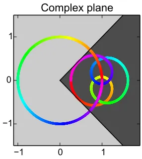
Figure 1: An example of polynomial q that satisfies our assumption. The unit circle is the collection of the in-puts of q and the other curve shows the corresponding outputs (with the corresponding colors.) We see the image of the polynomial stays in the wedge which contains all the com-plex number z satisfying <(q(z)) >
|=(q(z))|. We will require the state transition matrix satisfy
that the image of the unit circle on the complex plane under the polynomial q is contained in the cone of complex numbers whose real part is larger than their absolute imaginary part. Formally, for allz∈Csuch
that |z| = 1, we require that <(q(z)) > |=(q(z))|. Here, <(z) and =(z) denote the real and imaginary part of z, respectively. We illustrate this condition in Figure 1 on the right for a degree 4 system.
Our assumption has three important implica-tions. First, it implies (via Rouch´e’s theorem) that the spectral radius of Ais smaller than 1 and there-fore ensures the stability of the system. Second, the vectors satisfying our assumption form a convex set inRn.Finally, it ensures that the objective function
isweakly quasi-convex, a condition we introduce later when we show that it enables stochastic gradient de-scent to make sufficient progress.
We note in passing that our assumption can be satisfied via the `1-norm constraint kak1 ≤
√
2/2. Moreover, if we pick random Gaussian coefficients with expected norm bounded by o(1/√logn), then the resulting vector will satisfy our assumption with probability 1−o(1). Roughly speaking, the assump-tion requires the roots of the characteristic
polyno-mial p(z) = zn+a1zn−1 +· · ·+an are relatively dispersed inside the unit circle. (For comparison, on the other end of the spectrum, the polynomial p(z) = (z−0.99)n have all its roots colliding at the same point and doesn’t satisfy the assumption.)
Theorem 1.1 (Informal) Under our assumption, projected stochastic gradient descent, when givenN sample sequence of length T, returns parameters Θb with population risk
Ef(Θ)b ≤f(Θ) +O r
n5+σ2n3
T N
!
.
independence of the outputs as these are correlated by a common hidden state. The stated version of our result glosses over the fact that we need our assumption to hold with a small amount of slack; a precise version follows in Section 4. Our theorem establishes a polyno-mial convergence rate for stochastic gradient descent. Since each iteration of the algorithm only requires a sequence of matrix operations and an efficient projection step, the running time is polynomial, as well. Likewise, the sample requirements are polynomial since each iteration requires only a single fresh example. An important feature of this result is that the error decreases with both the lengthT and the number of samples N. The dependency on the dimension n, on the other hand, is likely to be quite loose, and tighter bounds are left for future work.
The algorithm requires a (polynomial-time) projection step to a convex set at every iteration (formally defined in Section 4 and Algorithm 1). Computationally, it can be a bottleneck, although it is unlikely to be required in practice and may be an artifact of our analysis.
1.3 The power of over-parameterization
Endowing the model with additional parameters compared to the ground truth turns out to be surprisingly powerful. We show that we can essentially remove the assumption we previously made in proper learning. The idea is simple. Ifpis the characteristic polynomial of A of degree n. We can find a system of order n0 > n such that the characteristic polynomial of its transition matrix becomes p·p0 for some polynomial p0 of order n0 −n. This means that to apply our result we only need the polynomial p ·p0 to satisfy our assumption. At this point, we can choosep0 to be an approximation of the inversep−1. For
sufficiently good approximation, the resulting polynomial p·p0 is close to 1 and therefore satisfies our assumption. Such an approximation exists generically forn0 =O(n) under mild non-degeneracy assumptions on the roots ofp. In particular, any small random perturbation of the roots would suffice.
Theorem 1.2 (Informal) Under a mild non-degeneracy assumption, stochastic gradient descent returns parameters Θb corresponding to a system of ordern0=O(n)with population risk
f(Θ)b ≤f(Θ) +O r
n5+σ2n3
T N
!
,
when givenN sample sequences of length T.
We remark that the idea we sketched also shows that, in the extreme, improper learning of linear dynamical systems becomes easy in the sense that the problem can be solved using linear regression against the outputs of the system. However, our general result interpolates between the proper case and the regime where linear regression works. We discuss in more details in Section 6.3.
1.4 Multi-input multi-output systems
(MIMO) systems is more delicate. Specifically, our results carry over to a broad family of multi-input multi-output systems. However, in general MIMO systems no longer enjoy canonical forms like SISO systems. In Section 7, we introduce a natural generalization of controllable canonical form for MIMO systems and extend our results to this case.
1.5 Related work
System identification is a core problem in dynamical systems and has been studied in depth for many years. The most popular reference on this topic is the text by Ljung Ljung (1998). Nonetheless, the list of non-asymptotic results on identifying linear systems from noisy data is surprisingly short. Several authors have recently tried to estimate the sample complexity of dynamical system identification using machine learning tools Vidyasagar and Karandikar (2008); Campi and Weyer (2002); Weyer and Campi (1999). All of these result are rather pessimistic with sample complexity bounds that are exponential in the degree of the linear system and other relevant quantities. Contrastingly, we prove that gradient descent has an associated polynomial sample complexity in all of these parameters. Moreover, all of these papers only focus on how well empirical risk approximates the true population risk and do not provide guarantees about any algorithmic schemes for minimizing the empirical risk.
The only result to our knowledge which provides polynomial sample complexity for identifying linear dynamical systems is in Shahet al Shah et al. (2012). Here, the authors show that if certain frequency domain information about the linear dynamical system is observed, then the linear system can be identified by solving a second-order cone program-ming problem. This result is about improper learning only, and the size of the resulting system may be quite large, scaling as the (1−ρ(A))−2. As we describe in this work, very
simple algorithms work in the improper setting when the system degree is allowed to be polynomial in (1−ρ(A))−1. Moreover, it is not immediately clear how to translate the frequency-domain results to the time-domain identification problem discussed above.
1.6 Proof overview
The first important step in our proof is to develop population risk in Fourier domain where it is closely related to what we call idealized risk. Idealized risk essentially captures the `2-difference between the transfer function of the learned system and the ground truth.
The transfer function is a fundamental object in control theory. Any linear system is completely characterized by its transfer function G(z) = C(zI−A)−1B. In the case of a SISO, the transfer function is a rational function of degree n over the complex numbers and can be written as G(z) =s(z)/p(z). In the canonical form introduced in Section 1.7, the coefficients of p(z) are precisely the parameters that specify A. Moreover, znp(1/z) = 1 +a1z+a2z2+· · ·+anzn is the polynomial we encountered in the introduction. Under the assumption illustrated earlier, we show in Section 3 that the idealized risk isweakly quasi-convex (Lemma 3.3). Quasi-convexity implies that gradients cannot vanish except at the optimum of the objective function; we review this (mostly known) material in Section 2. In particular, this lemma implies that in principle we can hope to show that gradient descent converges to a global optimum. However, there are several important issues that we need to address. First, the result only applies to idealized risk, not our actual population risk objective. Therefore it is not clear how to obtain unbiased gradients of the idealized risk objective. Second, there is a subtlety in even defining a suitable empirical risk objective. The reason is that risk is defined with respect to the correct initial state of the system which we do not have access to during training. We overcome both of these problems. In particular, we design an almost unbiased estimator of the gradient of the idealized risk in Lemma 5.4 and give variance bounds of the gradient estimator (Lemma 5.5).
Our results on improper learning in Section 6 rely on a surprisingly simple but powerful insight. We can extend the degree of the transfer functionG(z) by extending both numerator and denominator with a polynomial u(z) such that G(z) =s(z)u(z)/p(z)u(z). While this results in an equivalent system in terms of input-output behavior, it can dramatically change the geometry of the optimization landscape. In particular, we can see that only p(z)u(z) has to satisfy the assumption of our proper learning algorithm. This allows us, for example, to put u(z) ≈ p(z)−1 so that p(z)u(z) ≈ 1, hence trivially satisfying our assumption. A suitable inverse approximation exists under light assumptions and requires degree no more than d = O(n). Algorithmically, there is almost no change. We simply run stochastic gradient descent withn+dmodel parameters rather than nmodel parameters.
1.7 Preliminaries
For complex matrix (or vector, number) C, we use <(C) to denote the real part and =(C) the imaginary part, and ¯C the conjugate andC∗ = ¯C>its conjugate transpose . We use | · |
to denote the absolute value of a complex number c. For complex vector u and v, we use
hu, vi= u∗v to denote the inner product and kuk =√u∗u is the norm of u. For complex
matrix A and B with same dimension, hA, Bi = tr(A∗B) defines an inner product, and
kAkF =ptr(A∗A) is the Frobenius norm. For a square matrixA, we use ρ(A) to denote
A SISO of order nis incontrollable canonical form ifA andB have the following form
A =
0 1 0 · · · 0
0 0 1 · · · 0
..
. ... ... . .. ...
0 0 0 · · · 1
−an −an−1 −an−2 · · · −a1
B=
0 0 .. . 0 1
(1.4)
We will parameterize ˆA,B,ˆ C,ˆ Dˆ accordingly. We will write A = CC(a) for brevity, where a is used to denote the unknown last row [−an, . . . ,−a1] of matrix A. We will use
ˆ
a to denote the corresponding training variables fora. Since here B is known, so ˆB is no longer a trainable parameter, and is forced to be equal to B. Moreover,C is a row vector and we use [c1,· · · , cn] to denote its coordinates (and similarly for ˆC).
A SISO iscontrollable if and only if the matrix [B |AB|A2B| · · · |An−1B] has rankn. This statement corresponds to the condition that all hidden states should be reachable from some initial condition and input trajectory. Any controllable system admits a controllable canonical form Heij et al. (2007). For vectora= [an, . . . , a1], letpa(z) denote the polynomial
pa(z) =zn+a1zn−1+· · ·+an. (1.5)
Whenadefines the matrixAthat appears in controllable canonical form, thenpais precisely the characteristic polynomial ofA.That is, pa(z) = det(zI−A).
2. Gradient descent and quasi-convexity
It is known that under certain mild conditions (stochastic) gradient descent converges even on non-convex functions to local minimum Ge et al. (2015); Lee et al. (2016). Though usu-ally for concrete problems the challenge is to prove that there is no spurious local minimum other than the target solution. Here we introduce a condition similar to the quasi-convexity notion in Hazan et al. (2015), which ensures that any point with vanishing gradient is the optimal solution . Roughly speaking, the condition says that at any pointθthe negative of the gradient −∇f(θ) should be positively correlated with directionθ∗−θpointing towards the optimum. Our condition is slightly weaker than that in Hazan et al. (2015) since we only require quasi-convexity and smoothness with respect to the optimum, and this (simple) extension will be necessary for our analysis.
Definition 2.1 (Weak quasi-convexity) We say an objective function f is τ -weakly-quasi-convex (τ-WQC) over a domain B with respect to global minimum θ∗ if there is a positive constant τ >0 such that for all θ∈ B,
∇f(θ)>(θ−θ∗)≥τ(f(θ)−f(θ∗)). (2.1)
We further sayf is Γ-weakly-smooth if for for any point θ, k∇f(θ)k2 ≤Γ(f(θ)−f(θ∗)).
Note that indeed any Γ-smooth function in the usual sense (that is, k∇2fk ≤ Γ) is O
(Γ)-weakly-smooth. For a random vector X ∈ Rn, we define it’s variance to be Var[X] =
Definition 2.2 We callr(θ) an unbiased estimator of∇f(θ) with varianceV if it satisfies E[r(θ)] =∇f(θ) and Var[r(θ)]≤V.
Projected stochastic gradient descent over some closed convex setBwithlearning rateη > 0 refers to the following algorithm in which ΠB denotes the Euclidean projection ontoB:
fork= 0 to K−1 : wk+1 =θk−ηr(θk)
θk+1 = ΠB(wk+1)
return θj withj uniformly picked from 1, . . . , K (2.2)
The following Proposition is well known for convex objective functions (corresponding to 1-weakly-quasi-convex functions). We extend it (straightforwardly) to the case when τ-WQC holds with any positive constantτ.
Proposition 2.3 Suppose the objective function f isτ-weakly-quasi-convex and Γ -weakly-smooth, and r(·) is an unbiased estimator for ∇f(θ) with variance V. Moreover, suppose the global minimum θ∗ belongs to B, and the initial point θ0 satisfieskθ0−θ∗k ≤R. Then projected gradient descent (2.2)with a proper learning rate returnsθK in K iterations with expected error
Ef(θK)−f(θ∗)≤O max (
ΓR2 τ2K,
R√V
τ√K
)!
.
Remark 2.4 It’s straightforward to see (from the proof ) that the algorithm tolerates in-verse exponential bias, namely bias on the order ofexp(−Ω(n)), in the gradient estimator. Technically, supposeE[r(θ)] =∇f(θ)±ζ thenf(θK)≤O
maxnΓτ2RK2,R
√
V τ√K
o
+ poly(K)·ζ. Throughout the paper, we assume that the error that we are shooting for is inverse poly-nomial, namely 1/nC for some absolute constant C, and therefore the effect of inverse exponential bias is negligible.
We defer the proof of Proposition 2.3 to Appendix A which is a simple variation of the standard convergence analysis of stochastic gradient descent (see, for example, Bottou (1998)). Finally, we note that the sum of two quasi-convex functions may no longer be quasi-convex. However, if a sequence functions is τ-WQC with respect to a common point θ∗, then their sum is also τ-WQC. This follows from the linearity of gradient operation.
Proposition 2.5 Suppose functions f1, . . . , fn are individually τ-weakly-quasi-convex in B with respect to a common global minimum θ∗ , then for non-negative w1, . . . , wn the linear combinationf =Pni=1wifi is also τ-weakly-quasi-convex with respect to θ∗ in B.
3. Population risk in frequency domain
of the objective function is fairly straightforward; we justify it toward the end of the section. We can show that
f(Θ)b ≈ kD−Dˆk2+ P∞
k=0 CˆAˆkB−CAkB 2
. (3.1)
The leading termkD−Dˆk2 is convex in ˆDwhich appears nowhere else in the objective.
It therefore doesn’t affect the convergence of the algorithm (up to lower order terms) by virtue of Proposition 2.5, and we restrict our attention to the remaining terms.
Definition 3.1 (Idealized risk) We define the idealized risk as
g( ˆA,Cˆ) =
∞
X
k=0
ˆ
CAˆkB−CAkB
2
. (3.2)
We now use basic concepts from control theory (see Heij et al. (2007); Hespanha (2009) for more background) to express the idealized risk (3.2) in Fourier domain. The transfer function of the linear system is
G(z) =C(zI−A)−1B . (3.3)
Note that G(z) is a rational function over the complex numbers of degree nand hence we can find polynomialss(z) andp(z) such that G(z) = ps((zz)),with the convention that the leading coefficient ofp(z) is 1. In controllable canonical form (1.4), the coefficients ofp will correspond to the last row of the A,while the coefficients of scorrespond to the entries of C. Also note that
G(z) =
∞
X
t=1
z−tCAt−1B =
∞
X
t=1
z−trt−1
The sequence r = (r0, r1, . . . , rt, . . .) = (CB, CAB, . . . , CAtB, . . .) is called the impulse response of the linear system. The behavior of a linear system is uniquely determined by the impulse response and therefore by G(z).Analogously, we denote the transfer function of the learned system by Gb(z) = ˆC(zI−Aˆ)−1B = ˆs(z)/pˆ(z). The idealized risk (3.2) is only a function of the impulse response ˆr of the learned system, and therefore it is only a function of Gb(z).
Recall that C= [c1, . . . , cn] is defined in Section 1.7. For future reference, we note that by some elementary calculation (see Lemma B.1), we have
G(z) =C(zI−A)−1B = c1+· · ·+cnz n−1
zn+a
1zn−1+· · ·+an
, (3.4)
which implies that s(z) =c1+· · ·+cnzn−1 andp(z) =zn+a1zn−1+· · ·+an.
With these definitions in mind, we are ready to express idealized risk in Fourier domain.
Proposition 3.2 Suppose pˆa(z) has all its roots inside unit circle, then the idealized risk
g(ˆa,Cˆ) can be written in the Fourier domain as
g( ˆA,Cˆ) = Z 2π
0 Gb(e
iθ)−G(eiθ) 2
Proof Note that G(eiθ) is the Fourier transform of the sequence{rk} and so isGb(eiθ) the Fourier transform2 of ˆrk. Therefore by Parseval’ Theorem, we have that
g( ˆA,Cˆ) =
∞
X
k=0
kˆrk−rkk2 = Z 2π
0
|Gb(eiθ)−G(eiθ)|2dθ . (3.5)
3.1 Quasi-convexity of the idealized risk
Now that we have a convenient expression for risk in Fourier domain, we can prove that the idealized riskg( ˆA,Cˆ) is weakly-quasi-convex when ˆais not so far from the trueain the sense thatpa(z) and ˆpa(z) have an angle less thanπ/2 for everyzon the unit circle. We will use the convention that aand ˆarefer to the parameters that specifyA and ˆA,respectively.
Lemma 3.3 For τ > 0 and every Cˆ, the idealized risk g( ˆA,Cˆ) is τ-weakly-quasi-convex over the domain
Nτ(a) =
ˆ
a∈Rn:<
pa(z)
pˆa(z)
≥τ /2,∀ z∈C, s.t.|z|= 1
. (3.6)
Proof We first analyze a single term h =|Gb(z)−G(z)|2. Recall that Gb(z) = ˆs(z)/pˆ(z) where ˆp(z) =paˆ(z) =zn+ ˆa1zn−1+· · ·+ ˆan. Note thatz is fixed and h is a function of ˆa and ˆC. Then it is straightforward to see that
∂h
∂ˆs(z) = 2<
1 ˆ p(z)
ˆ s(z) ˆ p(z) −
s(z) p(z)
∗
. (3.7)
and
∂h
∂pˆ(z) =−2<
ˆ s(z) ˆ p(z)2
ˆ s(z) ˆ p(z)−
s(z) p(z)
∗
. (3.8)
Since ˆs(z) and ˆp(z) are linear in ˆC and ˆarespectively, by chain rule we have that
h∂h
∂aˆ,ˆa−ai+h ∂h
∂Cˆ, ˆ
C−Ci= ∂h ∂pˆ(z)h
∂pˆ(z)
∂aˆ ,aˆ−ai+ ∂h ∂sˆ(z)h
∂ˆs(z)
∂Cˆ , ˆ C−Ci
= ∂h
∂pˆ(z)(ˆp(z)−p(z)) + ∂h
∂sˆ(z)(ˆs(z)−s(z)).
2. The Fourier transform exists sincekrkk2=kCˆAˆkBˆk2≤ kCˆkkAˆkkkBˆk ≤cρ( ˆA)kwherecdoesn’t depend
Plugging the formulas (3.7) and (3.8) for ∂∂hsˆ(z) and ∂∂hpˆ(z) into the equation above, we obtain that
h∂h
∂ˆa,ˆa−ai+h ∂h
∂Cˆ, ˆ
C−Ci= 2<
− ˆ
s(z)(ˆp(z)−p(z)) + ˆp(z)(ˆs(z)−s(z)) ˆ
p(z)2
ˆ s(z) ˆ p(z) −
s(z) p(z)
∗
= 2<
ˆ
s(z)p(z)−s(z)ˆp(z) ˆ
p(z)2
ˆ s(z) ˆ p(z)−
s(z) p(z)
∗
= 2<
(
p(z) ˆ p(z)
ˆ s(z) ˆ p(z) −
s(z) p(z)
2)
= 2<
p(z) ˆ p(z)
Gb(z)−G(z) 2
.
Hence h =|Gb(z)−G(z)|2 is τ-weakly-quasi-convex with τ = 2 min|z|=1< np(z)
ˆ p(z)
o . This implies our claim, since by Proposition 3.2, the idealized risk g is convex combination of functions of the form |Gb(z)−G(z)|2 for |z| = 1. Moreover, Proposition 2.5 shows that convex combination preserves weak quasi-convexity.
For future reference, we also prove that the idealized risk is O(n2/τ4
1)-weakly smooth. Lemma 3.4 The idealized risk g( ˆA,Cˆ) is Γ-weakly smooth withΓ =O(n2/τ14).
Proof By equation (3.8) and the chain rule we get that
∂g
∂Cˆ =
Z
T
∂|Gb(z)−G(z)|2
∂p(z) · ∂p(z)
∂Cˆ dz =
Z T 2< 1 ˆ p(z)
ˆ s(z) ˆ p(z) −
s(z) p(z)
∗
·[1, . . . , zn−1]dz .
therefore we can bound the norm of the gradient by
∂g ∂Cˆ
2 ≤ Z T ˆ s(z) ˆ p(z) −
s(z) p(z) 2 dz ! · Z T
4k[1, . . . , zn−1]k2· | 1
p(z)|
2dz
≤O(n/τ12)·g( ˆA,Cˆ).
Similarly, we could show that
∂g ∂ˆa 2
≤O(n2/τ12)·g( ˆA,Cˆ).
3.2 Justifying idealized risk
We need to justify the approximation we made in Equation (3.1).
Lemma 3.5 Assume that ξt and xt are drawn i.i.d. from an arbitrary distribution with mean0 and variance 1.Then the population risk f(Θ)b can be written as,
f(Θ) = ( ˆb D−D)2+ T−1 X
k=1
1− k
T
ˆ
The idealized risk is upper bound of the population risk f(Θ) according to equation (3.1)b and (3.9). We don’t have to quantify the gap between them because later in Algorithm 1, we will directly optimize the idealized risk by constructing an estimator of its gradient, and thus the optimization will guarantee a bounded idealized risk which translates to a bounded population risk. See Section 5 for details.
Proof [Proof of Lemma 3.5] Under the distributional assumptions on ξt and xt, we can calculate the objective functions above analytically. We write out yt,yˆt in terms of the inputs,
yt=Dxt+ t−1 X
k=1
CAt−k−1Bxk+CAt−1h0+ξt, yˆt= ˆDxt+ t−1 X
k=1
ˆ
CAˆt−k−1Bxˆ k+CAt−1h0.
Therefore, using the fact that xt’s are independent and with mean 0 and covariance I, the expectation of the error can be calculated (formally by Claim B.2),
E
kyˆt−ytk2
=kDˆ−Dk2 F +
Pt−1 k=1
CˆAˆt−k−1Bˆ−CAt−k−1B 2
F +E[kξtk
2]. (3.10)
UsingE[kξtk2] =σ2,it follows that
f(Θ) =b kDˆ −Dk2F +PT
−1 k=1 1−Tk
CˆAˆk−1Bˆ−CAk−1B 2 F +σ
2. (3.11)
Recall that under the controllable canonical form (1.4), B = en is known and therefore ˆ
B =B is no longer a variable. Then the expected objective function (3.11) simplifies to
f(Θ) = ( ˆb D−D)2+PT
−1 k=1 1− Tk
ˆ
CAˆk−1B−CAk−1B2 +σ2.
The previous lemma does not yet control higher order contributions present in the idealized risk. This requires additional structure that we introduce in the next section.
4. Effective relaxations of spectral radius
The previous section showed quasi-convexity of the idealized risk. However, several steps are missing towards showing finite sample guarantees for stochastic gradient descent. In particular, we will need to control the variance of the stochastic gradient at any system that we encounter in the training. For this purpose we formally introduce our main assumption now and show that it serves as an effective relaxation of spectral radius. This results below will be used for proving convergence of stochastic gradient descent in Section 5.
Consider the following convex region C in the complex plane,
C={z:<z≥(1 +τ0)|=z|} ∩ {z:τ1<<z < τ2}. (4.1)
where τ0, τ1, τ2 > 0 are constants that are considered as fixed constant throughout the
paper. Our bounds will have polynomial dependency on these parameters. Pictorially, this convex set is pretty much the dark area in Figure 1 (with the corner chopped). This set in
C induces a convex set in the parameter space which is a subset of the transition matrix
Definition 4.1 We say a polynomial p(z) is α-acquiescent if {p(z)/zn:|z| = α} ⊆ C. A linear system with transfer function G(z) =s(z)/p(z) is α-acquiescent if the denominator
p(z) is.
The set of coefficientsa∈Rn defining acquiescent systems form a convex set. Formally,
for a positiveα >0, define the convex setBα ⊆Rn as
Bα=
a∈Rn:{pa(z)/zn:|z|=α} ⊆ C . (4.2)
We note that definition (4.2) is equivalent to the definitionBα=
a∈Rn:{znp(1/z) :|z|= 1/α} ⊆ C , which is the version that we used in introduction for simplicity. Indeed, we can verify the convexity of Bα by definition and the convexity of C: a, b∈Bα implies that
pa(z)/zn, pb(z)/zn ∈ C and therefore, p(a+b)/2(z)/zn = 12(pa(z)/z n +p
b(z)/zn) ∈ C. We also note that the parameterαin the definition of acquiescence corresponds to the spectral radius of the companion matrix. In particular, an acquiescent system is stable forα <1.
Lemma 4.2 Suppose a∈ Bα, then the roots of polynomialpa(z) have magnitudes bounded by α. Therefore the controllable canonical formA= CC(a) defined by a has spectral radius
ρ(A)< α.
Proof Define holomorphic function f(z) =zn andg(z) =pa(z) =zn+a1zn−1+· · ·+an. We apply the symmetric form of Rouche’s theorem Estermann (1962) on the circle K =
{z : |z|= α}. For any point z on K, we have that |f(z)|= αn, and that |f(z)−g(z)|= αn· |1−pa(z)/zn|. Sincea∈ Bα, we have thatpa(z)/zn∈ Cfor anyzwith|z|=α. Observe that for anyc∈ C we have that|1−c|<1 +|c|, therefore we have that
|f(z)−g(z)|=αn|1−pa(z)/zn|< αn(1 +|pa(z)|/|zn|) =|f(z)|+|pa(z)|=|f(z)|+|g(z)|.
Hence, using Rouche’s Theorem, we conclude that f and g have same number of roots inside circleK. Note that functionf =zn has exactlynroots inKand thereforeghave all its nroots inside circle K.
The following lemma establishes the fact thatBαis a monotone family of sets inα. The proof follows from the maximum modulo principle of the harmonic functions <(znp(1/z)) and =(znp(1/z)). We defer the short proof to Section C.1. We remark that there are larger convex sets than Bα that ensure bounded spectral radius. However, in order to also guarantee monotonicity and the no blow-up property below, we have to restrict our attention toBα.
Lemma 4.3 (Monotonicity of Bα) For any 0< α < β, we have that Bα ⊂ Bβ.
Our next lemma entails that acquiescent systems have well behaved impulse responses.
Lemma 4.4 (No blow-up property) Suppose a∈ Bα for some α ≤1. Then the com-panion matrix A= CC(a) satisfies
∞
X
k=0
Moreover, it holds that for any k≥0,
kAkBk2≤min{2πn/τ12,2πnα2k−2n/τ12}.
Proof [Proof of Lemma 4.4]
Letfλ =P∞k=0eiλkα−kAkB be the Fourier transform of the seriesα−kAkB. Then using
Parseval’s Theorem, we have
∞
X
k=0
kα−kAkBk2= Z 2π
0
|fλ|2dλ= Z 2π
0
|(I−α−1eiλA)−1B|2dλ
= Z 2π
0
Pn j=1α2j
|pa(αe−iλ)|2
dλ≤
Z 2π 0
n
|pa(αe−iλ)|2
dλ. (4.4)
where at the last step we used the fact that (I−wA)−1B = pa(w1−1)[w
−1, w−2. . . , z−n]>
(see Lemma B.1), and that α ≤ 1. Since a ∈ Bα, we have that |qa(α−1eiλ)| ≥ τ1, and
therefore pa(αe−iλ) =αne−inλq(eiλ/α) has magnitude at least τ1αn. Plugging in this into
equation (4.4), we conclude that
∞
X
k=0
kα−kAkBk2 ≤
Z 2π 0
n
|pa(αe−iλ)|2
dλ≤2πnα−2n/τ12.
Finally we establish the bound for kAkBk2. By Lemma 4.3, we have B
α ⊂ B1 forα ≤1.
Therefore we can pick α= 1 in equation (4.3) and it still holds. That is, we have that
∞
X
k=0
kAkBk2 ≤2πn/τ12.
This also implies thatkAkBk2≤2πn/τ2 1.
4.1 Efficiently computing the projection
In our algorithm, we require a projection onto Bα. However, the only requirement of the projection step is that it projects onto a set contained inside Bα that also contains the true linear system. So a variety of subroutines can be used to compute this projection or an approximation. First, the explicit projection onto Bα is representable by a semidefinite program. This is because each of the three constrains can be checked by testing if a trigono-metric polynomial is non-negative. A simple inner approximation can be constructed by requiring the constraints to hold on an a finite grid of size O(n). One can check that this provides a tight, polyhedral approximation to the set Bα, following an argument similar to Appendix C of Bhaskaret al Bhaskar et al. (2013). Projection to this polyhedral takes at most O(n3.5) time by linear programming and potentially can be made faster by using fast Fourier transform. See Section F for more detailed discussion on why projection on a polytope suffices. Furthermore, sometimes we can replace the constraint by an `1 or `2
5. Learning acquiescent systems
Next we show that we can learn acquiescent systems.
Theorem 5.1 Suppose the true system Θ is α-acquiescent and satisfies kCk ≤ 1. Then with N samples of length T ≥Ω(n+ 1/(1−α)), stochastic gradient descent (Algorithm 1) with projection set Bα returns parameters Θ = ( ˆb A,B,ˆ C,ˆ Dˆ) with population risk
Ef(Θ)b ≤f(Θ) +O
n2 N +
r
n5+σ2n3
T N
!
, (5.1)
whereO(·)-notation hides polynomial dependencies on1/(1−α),1/τ0,1/τ1, τ2, andR=kak. The expectation is taken over the randomness of the algorithms and the examples.
Algorithm 1 Projected stochastic gradient descent with partial loss
For i= 0 to N:
1. Take a fresh sample ((x1, . . . , xT),(y1, . . . , yT)). Let ˜yt be the simulated outputs3 of systemΘ on inputsb x and initial states h0 = 0.
2. Let T1 = T /4. Run stochastic gradient descent4 on loss function `((x, y),Θ) =b 1
T−T1 P
t>T1ky˜t−ytk
2. Concretely, let G
A = ∂`∂ˆa, GC = ∂∂`Cˆ, and , GD = ∂∂`Dˆ, we
update
[ˆa,C,ˆ Dˆ]→[ˆa,C,ˆ Dˆ]−η[GA, GC, GD].
3. Project Θ = (ˆb a,C,ˆ Dˆ) to the setBα⊗Rn⊗R.
Recall that T is the length of the sequence andN is the number of samples. The first term in the bound (5.1) comes from the smoothness of the population risk and the second comes from the variance of the gradient estimator of population risk (which will be described in detail below). An important (but not surprising) feature here is the variance scale in 1/T and therefore for long sequence actually we got 1/N convergence instead of 1/√N (for relatively smallN).
Computational complexity: Step 2 in each iteration of the algorithm takesO(T n) arithmetic operations, and the projection step takes O(n3.5) time to solve an linear programming problem. The project step is unlikely to be required in practice and may be an artifact of our analysis.
We can further balance the variance of the estimator with the number of samples by breaking each long sequence of length T into Θ(T /n) short sequences of length Θ(n), and then run back-propagation (1) on these T N/n shorter sequences. This leads us to the following bound which gives the right dependency in T and N as we expected: T N should be counted as the true number of samples for the sequence-to-sequence model.
4. Note that ˜yt is different from ˆyt defined in equation (1.2) which is used to define the population risk:
here ˆyt is obtained from the (wrong) initial stateh0 = 0 while ˆyt is obtained from the correct initial
state.
Corollary 5.2 Under the assumption of Theorem 5.1, Algorithm 2 returns parameters Θb with population risk
Ef(Θ)b ≤f(Θ) +O r
n5+σ2n3
T N
!
,
whereO(·)-notation hides polynomial dependencies on1/(1−α),1/τ0,1/τ1, τ2, andR=kak.
Algorithm 2 Projected stochastic gradient descent for long sequences
Input: N samples sequences of lengthT
Output: Learned systemΘb
1. Divide each sample of lengthT intoT /(βn) samples of length βnwhere β is a large enough constant. Then run algorithm 1 with the new samples and obtain Θ.b
We remark the the gradient computation procedure takes time linear in T n since one can use chain-rule (also called back-propagation) to compute the gradient efficiently . For completeness, Algorithm 3 gives a detailed implementation. Finally and importantly, we remark that although we defined the population risk as the expected error with respected to sequence of length T, actually our error bound generalizes to any longer (or shorter) sequences of lengthT0 max{n,1/(1−α)}. By the explicit formula forf(Θ) (Lemma 3.5)b and the fact that kCAkBk decays exponentially for k n (Lemma 4.4), we can bound the population risk on sequences of different lengths. Concretely, let fT0(Θ) denote theb population risk on sequence of length T0, we have for all T0 max{n,1/(1−α)},
fT0(Θ)b ≤1.1f(Θ) + exp(b −(1−α) min{T, T0})≤O r
n5+σ2n3
T N
!
.
We note that generalization to longer sequence does deserve attention. Indeed in prac-tice, it’s usually difficult to train non-linear recurrent networks that generalize to longer sequences than the training data.
We could hope to achieve linear convergence by showing that the empirical risk also satisfies the weakly-quasi-convexity. Then, we can re-use the samples and hope to use strong optimization tools (such as SVRG) to achieve the linear convergence. This is beyond the scope of this paper and left to future work.
Our proof of Theorem 5.1 simply consists of three parts: a) showing the idealized risk is weakly quasi-convex in the convex set Bα (Lemma 5.3); b) designing an (almost) unbiased estimator of the gradient of the idealized risk (Lemma 5.4); c) variance bounds of the gradient estimator (Lemma 5.5).
First of all, using the theory developed in Section 3 (Lemma 3.3 and Lemma 3.4), it is straightforward to verify that in the convex setBα⊗Rn, the idealized risk is both
weakly-quasi-convex and weakly-smooth.
Lemma 5.3 Under the condition of Theorem 5.1, the idealized risk (3.2)isτ -weakly-quasi-convex in the -weakly-quasi-convex set Bα⊗Rn and Γ-weakly smooth, where τ = Ω(τ0τ1/τ2) and Γ =
Proof[Proof of Lemma 5.3] It suffices to show that for all ˆa, a∈ Bα, it satisfies ˆa∈ Nτ(a) for τ = Ω(τ0τ1/τ2). Indeed, by the monotonicity of the family of setsBα (Lemma 4.3), we have that ˆa, a∈ B1, which by definition means for everyzon unit circle, pa(z)/zn, paˆ(z)/zn∈ C.
By definition ofC, for any pointw,wˆ∈ C, the angleφbetweenwand ˆwis at mostπ−Ω(τ0)
and ratio of the magnitude is at leastτ1/τ2, which implies that<(w/wˆ) =|w|/|wˆ| ·cos(φ)≥
Ω(τ0τ1/τ2). Therefore <(pa(z)/pˆa(z))≥Ω(τ0τ1/τ2), and we conclude that ˆa∈ Nτ(a). The smoothness bound was established in Lemma 3.4.
Towards designing an unbiased estimator of the gradient, we note that there is a small caveat here that prevents us to just use the gradient of the empirical risk, as commonly done for other (static) problems. Recall that the population risk is defined as the expected risk with known initial state h0, while in the training we don’t have access to the initial
states and therefore using the naive approach we couldn’t even estimate population risk from samples without knowing the initial states.
We argue that being able to handle the missing initial states is indeed desired: in most of the interesting applicationsh0 is unknown (or even to be learned). Moreover, the ability
of handling unknown h0 allows us to break a long sequence into shorter sequences, which
helps us to obtain Corollary 5.2. Here the difficulty is essentially that we have a supervised learning problem with missing datah0. We get around it by simply ignoring firstT1= Ω(T)
outputs of the system and setting the corresponding errors to 0. Since the influence ofh0to
any outputs later than timek≥T1max{n,1/(1−α)}is inverse exponentially small, we
could safely assume h0 = 0 when the error earlier than timeT1 is not taken into account.
This small trick also makes our algorithm suitable to the cases when these early outputs are actually not observed. This is indeed an interesting setting, since in many sequence-to-sequence model Sutskever et al. (2014), there is no output in the first half fraction of iterations (of course these models have non-linear operation that we cannot handle).
The proof of the correctness of the estimator is almost trivial and deferred to Section C.
Lemma 5.4 Under the assumption of Theorem 5.1, suppose ˆa, a ∈ Bα. Then in Algo-rithm 1, at each iteration, GA, GC are unbiased estimators of the gradient of the idealized risk (3.2)in the sense that:
E[GA, GC] =
∂g ∂aˆ,
∂g
∂Cˆ
±exp(−Ω((1−α)T)).
(5.2)
Finally, we control the variance of the gradient estimator.
Lemma 5.5 The (almost) unbiased estimator(GA, GC)of the gradient ofg( ˆA,Cˆ)has vari-ance bounded by
Var [GA] + Var [GC]≤
O n3Λ2/τ16+σ2n2Λ/τ14
T .
Note that Lemma 5.5 does not directly follow from the Γ-weakly-smoothness of the population risk, since it’s not clear whether the loss function`((x, y),Θ) is also Γ-smooth forb every sample. Moreover, even if it could work out, from smoothness the variance bound can be only as small as Γ2, while the true variance scales linearly in 1/T. Here the discrepancy comes from that smoothness implies an upper bound of the expected squared norm of the gradient, which is equal to the variance plus the expected squared mean. Though typically for many other problems variance is on the same order as the squared mean, here for our sequence-to-sequence model, actually the variance decreases in length of the data, and therefore the bound of variance from smoothness is pessimistic.
We bound directly the variance instead. It’s tedious but simple in spirit. We mainly need Lemma 4.4 to control various difference sums that shows up from calculating the expectation. The only tricky part is to obtain the 1/T dependency which corresponds to the cancellation of the contribution from the cross terms. In the proof we will basically write out the variance as a (complicated) function of ˆA,Cˆ which consists of sums of terms involving ( ˆCAˆkB−CAkB) and ˆAkB. We control these sums using Lemma 4.4. The proof is deferred to Section C.
Finally we are ready to prove Theorem 5.1. We essentially just combine Lemma 5.3, Lemma 5.4 and Lemma 5.5 with the generic convergence Proposition 2.3. This will give us low error in idealized risk and then we relate the idealized risk to the population risk.
Proof [Proof of Theorem 5.1] We consider g0( ˆA,C,ˆ Dˆ) = ( ˆD −D)2 + g( ˆA,Cˆ), an ex-tended version of the idealized risk which takes the contribution of ˆD into account. By Lemma 5.4 we have that Algorithm 1 computes GA, GC which are almost unbiased esti-mators of the gradients of g0 up to negligible error exp(−Ω((1−α)T)), and by Lemma C.2 we have GD is an unbiased estimator of g0 with respect to ˆD. Moreover by Lemma 5.5,
these unbiased estimator has total variance V = O(n 5+σ2n3)
T where O(·) hides dependency on τ1 and (1−α). Applying Proposition 2.3 (which only requires an unbiased
estima-tor of the gradient of g0), we obtain that after T iterations, we converge to a point with
g0(ˆa,C,ˆ Dˆ)≤O
n2 N +
q
n5+σ2n3 T N
. Then, by Lemma 3.5 we havef(Θ)b ≤g0(ˆa,C,ˆ Dˆ)+σ2=
g0(ˆa,C,ˆ Dˆ) +f(Θ)≤O
n2 N +
q
n5+σ2n3 T N
+f(Θ) which completes the proof.
6. The power of improper learning
We observe an interesting and important fact about the theory in Section 5: it solely requires a condition on the characteristic functionp(z). This suggests that the geometry of the training objective function depends mostly on the denominator of the transfer function, even though the system is uniquely determined by the transfer function G(z) =s(z)/p(z). This might seem to be an undesirable discrepancy between the behavior of the system and our analysis of the optimization problem.
coefficient 1, we can write G(z) as
G(z) = s(z)u(z) p(z)u(z) =
˜ s(z)
˜ p(z),
where ˜s = su and ˜p = pu. Therefore the system ˜s(z)/p˜(z) has identical behavior as G. Although this is a redundant representation of G(z), it should counted as an acceptable solution. After all, learning the minimum representation5 of linear system is impossible in general. In fact, we will encounter an example in Section 6.1.
While not changing the behavior of the system, the extension fromp(z) to ˜p(z),does af-fect the geometry of the optimization problem. In particular, if ˜p(z) is now anα-acquiescent characteristic polynomial as defined in Definition 4.1, then we could find it simply using stochastic gradient descent as shown in Section 5. Observe that we don’t require knowledge of u(z) but only its existence. Denoting bydthe degree ofu, the algorithm itself is simply stochastic gradient descent with n+dmodel parameters instead ofn.
Our discussion motivates the following definition.
Definition 6.1 A polynomial p(z) of degree n is α-acquiescent by extension of degree d
if there exists a polynomial u(z) of degree d and leading coefficient 1 such that p(z)u(z) is
α-acquiescent.
For a transfer function G(z), we define it’sH2 norm as
kGk2H
2 = 1 2π
Z 2π 0
|G(eiθ)|2dθ .
We assume (with loss of generality) that the true transfer function G(z) has bounded
H2 norm, that is, kGkH2 ≤1. This can be achieve by a rescaling
6 of the matrixC.
Theorem 6.2 Suppose the true system has transfer functionG(z) =s(z)/p(z)with a char-acteristic function p(z)that isα-acquiescent by extension of degreed, and kGkH2 ≤1, then
projected stochastic gradient descent with m = n+d states (that is, Algorithm 2 with m
states) returns a system Θb with population risk
f(Θ)b ≤O r
m5+σ2m3
T K
!
.
where theO(·) notation hides polynomial dependencies on τ0, τ1, τ2,1/(1−α).
The theorem follows directly from Corollary 5.2 (with some additional care about the scaling.
Proof [Proof of Theorem 6.2] Let ˜p(z) = p(z)u(z) be the acquiescent extension of p(z). Since τ2 ≥ |u(z)p(z)|=|p˜(z)| ≥τ0 on the unit circle, we have that |s˜(z)|=|s(z)||u(z)|=
5. The minimum representation of a transfer functionG(z) is defined as the representationG(z) =s(z)/p(z) withp(z) having minimum degree.
6. In fact, this is a natural scaling that makes comparing error easier. Recall that the population risk is essentiallykGˆ−GkH2, therefore rescalingCso thatkGkH2= 1 implies that when error1 we achieve
s(z)·Oτ(1/p(z)). Therefore we have that ˜s(z) satisfies thatk˜skH2 =Oτ(ks(z)/p(z)kH2) = Oτ(kG(z)kH2)≤Oτ(1). That means that the vector C that determines the coefficients of ˜
s satisfies that kCk ≤Oτ(1),since for a polynomial h(z) = b0 +· · ·+bn−1zn−1, we have
khkH2 =kbk.Therefore we can apply Corollary 5.2 to complete the proof.
In the rest of this section, we discuss in subsection 6.1 the instability of the minimum representation in subsection, and in subsection 6.2 we show several examples where the characteristic function p(z) is not α-acquiescent but is α-acquiescent by extension with small degree d.
As a final remark, the examples illustrated in the following sub-sections may be far from optimally analyzed. It is beyond the scope of this paper to understand the optimal condition under whichp(z) is acquiescent by extension.
6.1 Instability of the minimum representation
We begin by constructing a contrived example where the minimum representation ofG(z) is not stable at all and as a consequence one can’t hope to recover the minimum representation of G(z).
Consider G(z) = ps((zz)) := (z−0z.1)(n−z0n.8−−n0.9−n) and G0(z) = s0(z)
p0(z) := z−10.1. Clearly these are
the minimum representations of the G(z) and G0(z), which also both satisfy acquiescence. On the one hand, the characteristic polynomial p(z) and p0(z) are very different. On the other hand, the transfer functionsG(z) andG0(z) have almost the same values on unit circle up to exponentially small error,
|G(z)−G0(z)| ≤ 0.8
−n−0.9−n
(z−0.1)(z−0.9−n) ≤exp(−Ω(n)).
Moreover, the transfer functions G(z) and ˆG(z) are on the order of Θ(1) on unit circle. These suggest that from an (inverse polynomially accurate) approximation of the transfer functionG(z), we cannot hope to recover the minimum representation in any sense, even if the minimum representation satisfies acquiescence.
6.2 Power of improper learning in various cases
We illustrate the use of improper learning through various examples below.
6.2.1 Example: artificial construction
We consider a simple contrived example where improper learning can help us learn the transfer function dramatically. We will show an example of characteristic function which is not 1-acquiescent but (α+ 1)/2-(α+ 1)/2-acquiescent by extension of degree 3.
Letnbe a large enough integer andαbe a constant. LetJ ={1, n−1, n}andω=e2πi/n, and then definep(z) =z3Q
j∈[n],j /∈J(z−αωj). Therefore we have that
p(z)/zn=z3 Y
j∈[n],j∈J
(1−αωj/z) = 1−α
n/zn
Taking z = e−iπ/2 we have that p(z)/zn has argument (phase) roughly −3π/4, and therefore it’s not in C, which implies that p(z) is not 1-acquiescent. On the other hand, pickingu(z) = (z−ω)(z−1)(z−ω−1) as the helper function, from equation (6.1) we have p(z)u(z)/zn+3 = 1−αn/zn takes values inverse exponentially close to 1 on the circle with radius (α+ 1)/2. Thereforep(z)u(z) is (α+ 1)/2-acquiescent.
6.2.2 Example: characteristic function with separated roots
A characteristic polynomial with well separated roots will be acquiescent by extension. Our bound will depend on the following quantity ofpthat characterizes the separateness of the roots.
Definition 6.3 For a polynomial h(z) of degree n with roots λ1, . . . , λn inside unit circle, define the quantityΓ(·) of the polynomial h as:
Γ(h) := X j∈[n]
λnj
Q
i6=j(λi−λj)
.
Lemma 6.4 Suppose p(z) is a polynomial of degree nwith distinct roots inside circle with radiusα. LetΓ = Γ(p), thenp(z) isα-acquiescent by extension of degree d =O(max{(1−
α)−1log(√nΓ· kpk
H2),0}).
Our main idea to extend p(z) by multiplying some polynomial u that approximates p−1 (in a relatively weak sense) and therefore pu will always take values in the setC. We believe the following lemma should be known though for completeness we provide the proof in Section D.
Lemma 6.5 (Approximation of inverse of a polynomial) Suppose p(z) is a polyno-mial of degree n and leading coefficient 1 with distinct roots inside circle with radius α, and Γ = Γ(p). Then for d=O(max{(1−1αlog(1−Γα)ζ,0}), there exists a polynomial h(z) of degree dand leading coefficient 1 such that for all z on unit circle,
zn+d
p(z) −h(z)
≤ζ .
Proof [Proof of Lemma 6.4] Letγ = 1−α. Using Lemma 6.5 withζ = 0.5kpk−H1
∞, we have
that there exists polynomialu of degreed=O(max{ 1
1−αlog(ΓkpkH∞),0}) such that
zn+d
p(z) −u(z)
≤ζ .
Then we have that
p(z)u(z)/z
n+d−1
≤ζ|p(z)|<0.5.
Therefore p(z)u(z)/zn+d ∈ Cτ0,τ1,τ2 for constant τ0, τ1, τ2. Finally noting that for degreen polynomial we havekhkH∞ ≤
√
6.2.3 Example: Characteristic polynomial with random roots
We consider the following generative model for characteristic polynomial of degree 2n. We generate n complex numbers λ1, . . . , λn uniformly randomly on circle with radius α < 1, and take λi,λ¯i fori= 1, . . . , nas the roots ofp(z). That is,p(z) = (z−λ1)(z−λ¯1). . .(z−
λn)(z−λ¯n). We show that with good probability (over the randomness ofλi’s), polynomial
p(z) will satisfy the condition in subsection 6.2.2 so that it can be learned efficiently by our improper learning algorithm.
Theorem 6.6 Suppose p(z) with random roots inside circle of radius α is generated from the process described above. Then with high probability over the choice of p, we have that
Γ(p) ≤ exp(Oe(
√
n)) and kpkH2 ≤ exp( ˜O(
√
n)). As a corollary, p(z) is α-acquiescent by extension of degreeOe((1−α)−1n).
Towards proving Theorem 6.6, we need the following lemma about the expected distance of two random points with radiusρ and r in log-space.
Lemma 6.7 Let x ∈C be a fixed point with |x|=ρ, and λ uniformly drawn on the circle with radius r. Then E[ln|x−λ|] = ln max{ρ, r}.
Proof When r 6=ρ, let N be an integer andω =e2iπ/N. Then we have that
E[ln|x−λ| |r] = lim N→∞
1 N
N X
k=1
ln|x−rωk| (6.2)
The right hand of equation (6.2) can be computed easily by observing that N1 PNk=1ln|x−
rωk|= N1 ln
QN
k=1(x−rωk) =
1
N ln|xN−rN|. Therefore, whenρ > r, we have limN→∞ 1 N
PN
k=1ln|x−
rωk| = limN→∞ρ+ N1 ln|(x/ρ)N −(r/ρ)N| = lnρ. On the other hand, when ρ < r, we
have that limN→∞ N1 PNk=1ln|x−rωk| = lnr. Therefore we have that E[ln|x−λ| | r] =
ln(maxρ, r). For ρ=r, similarly proof (with more careful concern of regularity condition) we can show thatE[ln|x−λ| |r] = lnr.
Now we are ready to prove Theorem 6.6.
Proof [Proof of Theorem 6.6] Fixing indexi, and the choice ofλi, we consider the random variableYi= ln( |λi|
2n
Q
j6=i|λi−λj|Qj6=i|λi−λ¯j|)nln|λi| − P
j6=iln|λi−λj|. By Lemma 6.7, we have that E[Yi] = nln|λi| −Pj6=iE[ln|λi −λj|] = ln(1−δ). Let Zj = ln|λi −λj|. Then we have that Zj are random variable with mean 0 and ψ1-Orlicz norm bounded by 1 since E[eln|λi−λj|−1] ≤ 1. Therefore by Bernstein inequality for sub-exponential tail random
variable (for example, (Ledoux and Talagrand, 2013, Theorem 6.21)), we have that with high probability (1−n−10), it holds that
P j6=iZj
≤ Oe(
√
n) where Oe hides logarithmic
factors. Therefore, with high probability, we have |Yi| ≤Oe(
√
n).
Finally we take union bound over all i ∈ [n], and obtain that with high probability, for ∀i∈ [n],|Yi| ≤ Oe(
√
n), which implies that Pni=1exp(Yi) ≤ exp(Oe(
√
n)). With similar technique, we can prove that kpkH2 ≤exp( ˜O(
√
6.2.4 Example: Passive systems
We will show that with improper learning we can learn almost all passive systems, an important class of stable linear dynamical system as we discussed earlier. We start off with the definition of a strict-input passive system.
Definition 6.8 (Passive System, c.f Kottenstette and Antsaklis (2010)) A SISO lin-ear system is strict-input passive if and only if for some τ0 >0 and any z on unit circle,
<(G(z))≥τ0.
In order to learn the passive system, we need to add assumptions in the definition of strict passivity. To make it precise, we define the following subsets of complex plane: For positive constant τ0, τ1, τ2, define
Cτ+
0,τ1,τ2 ={z∈C:|z| ≤τ2,<(z)≥τ1,<(z)≥τ0|=(z)| }. (6.3) We say a transfer functionG(z) =s(z)/p(z) is (τ0, τ1, τ2)-strict input passive if for anyz
on unit circle we haveG(z)∈ C+
τ0,τ1,τ2. Note that for small constantτ0, τ1 and large constant τ2, this basically means the system is strict-input passive.
Now we are ready to state our main theorem in this subsection. We will prove that pas-sive systems could be learned improperly with a constant factor more states (dimensions), assumings(z) has all its roots strictly inside unit circles and Γ(s)≤exp(O(n)).
Theorem 6.9 Suppose G(z) =s(z)/p(z) is(τ0, τ1, τ2)-strict-input passive. Moreover, sup-pose the roots ofs(z)have magnitudes inside circle with radiusα andΓ = Γ(s)≤exp(O(n))
and kpkH2 ≤ exp(O(n)). Then p(z) is α-acquiescent by extension of degree d = Oτ,α(n),
and as a consequence we can learn G(z) with n+d states in polynomial time.
Moreover, suppose in addition we assume thatG(z)∈ Cτ0,τ1,τ2 for everyz on unit circle. Then p(z) isα-acquiescent by extension of degree d=Oτ,α(n).
The proof of Theorem 6.9 is similar in spirit to that of Lemma 6.4, and is deferred to Section D.
6.3 Improper learning using linear regression
In this subsection, we show that under stronger assumption thanα-acquiescent by extension, we can improperly learn a linear dynamical system with linear regression, up to some fixed bias.
The basic idea is to fit a linear function that maps [xk−`, . . . , xk] toyk. This is equivalent to a dynamical system with`hidden states and with the companion matrixAin (1.4) being chosen asa`= 1 and a`−1 =· · ·=a1= 0. In this case, the hidden states exactly memorize
all the previous`inputs, and the output is a linear combination of the hidden states. Equivalently, in the frequency space, this corresponds to fitting the transfer function G(z) =s(z)/p(z) with a rational function of the form c1z`−1+···+c1
z`−1 =c1z
Definition 6.10 A polynomial p(z) of degree n is extremely-acquiescent by extension of degree d with bias ε if there exists a polynomial u(z) of degree d and leading coefficient 1 such that for all z on unit circle,
p(z)u(z)/z
n+d−1
≤ε (6.4)
We remark that if p(z) is 1-acquiescent by extension of degree d, then there exists u(z) such that p(z)u(z)/zn+d ∈ C. Therefore, equation (6.4) above is a much stronger requirement than acquiescence by extension.7
When p(z) is extremely-acquiescent, we see that the transfer functionG(z) =s(z)/p(z) can be approximated bys(z)u(z)/zn+dup to biasε. Let`=n+d+1 ands(z)u(z) =c1z`−1+
· · ·+c`. Then we have thatG(z) can be approximated by the following dynamical system of
`hidden states withεbias: we chooseA= CC(a) witha` = 1 anda`−1=· · ·=a1 = 0, and
C= [c1, . . . , c`]. As we have argued previously, such a dynamical system simply memorizes all the previous`inputs, and therefore it is equivalent to linear regression from the feature [xk−`, . . . , xk] to output yk.
Proposition 6.11 (Informal) If the true system G(z) = s(z)/p(z) satisfies that p(z) is extremely-acquiescent by extension of degree d. Then using linear regression we can learn mapping from [xk−`, . . . , xk]to yk with bias ε and polynomial sampling complexity.
We remark that with linear regression the biasεwill only go to zero as we increase the length ` of the feature, but not as we increase the number of samples. Moreover, linear regression requires a stronger assumption than the improper learning results in previous subsections do. The latter can be viewed as an interpolation between the proper case and the regime where linear regression works.
7. Learning multi-input multi-output (MIMO) systems
We consider multi-input multi-output systems with the transfer functions that have a com-mon denominator p(z),
G(z) = 1
p(z) ·S(z) (7.1)
whereS(z) is an`in×`out matrix with each entry being a polynomial with real coefficients
of degree at most nandp(z) =zn+a1zn−1+· · ·+an. Note that here we use`into denote
the dimension of the inputs of the system and`out the dimension of the outputs.
Although a special case of a general MIMO system, this class of systems still contains many interesting cases, such as the transfer functions studied in Fazel et al. (2001, 2004), where G(z) is assumed to take the form G(z) =R0 +Pni=1
Ri
z−λi, for λ1, . . . , λn ∈C with
conjugate symmetry andRi∈C`out×`in satisfies thatRi = ¯Rj whenever λi= ¯λj.
In order to learn the systemG(z), we parametrizep(z) by its coefficientsa1, . . . , an and
S(z) by the coefficients of its entries. Note that each entry of S(z) depends on n+ 1 real
coefficients and therefore the collection of coefficients forms a third order tensor of dimension `out×`in×(n+ 1). It will be convenient to collect the leading coefficients of the entries of
S(z) into a matrix of dimension`out×`in, named D, and the rest of the coefficients into a
matrix of dimension `out×`inn, denoted byC. This will be particularly intuitive when a
state-space representation is used to learn the system with samples as discussed later. We parameterize the training transfer function ˆG(z) by ˆa, ˆC and ˆDusing the same way.
Let’s define the risk function in the frequency domain as,
g( ˆA,C,ˆ Dˆ) = Z 2π
0 G(e
iθ)−Gˆ(eiθ) 2
F dθ . (7.2)
The following lemma is an analog of Lemma 3.3 for the MIMO case. Itss proof actually follows from a straightforward extension of the proof of Lemma 3.3 by observing that matrix S(z) (or ˆS(z)) commute with scalarp(z) and ˆp(z), and that ˆS(z),pˆ(z) are linear in ˆa,Cˆ.
Lemma 7.1 The risk functiong(ˆa,Cˆ) defined in (7.2) isτ-weakly-quasi-convex in the do-main
Nτ(a) =
ˆ
a∈Rn:<
pa(z)
pˆa(z)
≥τ /2,∀ z∈C, s.t. |z|= 1
⊗R`in×`out×n 0
Finally, as alluded before, we use a particular state space representation for learning the system in time domain with example sequences. It is known that any transfer function of the form (7.1) can be realized uniquely by the state space system of the following special case of Brunovsky normal form Brunovsky (1970),
A =
0 I`in 0 · · · 0
0 0 I`in · · · 0
..
. ... ... . .. ...
0 0 0 · · · I`in
−anI`in −an−1I`in −an−2I`in · · · −a1I`in
, B =
0 .. . 0 I`in
, (7.3)
and,
C∈R`out×n`in, D∈
R`out×`in.
The following Theorem is a straightforward extension of Corollary 5.2 and Theorem 6.2 to the MIMO case.
Theorem 7.2 Suppose transfer function G(z) of a MIMO system takes form (7.1), and has norm kGkH2 ≤ 1. If the common denominator p(z) is α-acquiescent by extension of
degree dthen projected stochastic gradient descent over the state space representation (7.3)
will return Θb with risk
f(Θ)b ≤
poly(n+d, σ, τ,(1−α)−1)
T N .