Density Estimation in Infinite Dimensional Exponential
Families
Bharath Sriperumbudur bks18@psu.edu
Department of Statistics, Pennsylvania State University University Park, PA 16802, USA.
Kenji Fukumizu fukumizu@ism.ac.jp
The Institute of Statistical Mathematics
10-3 Midoricho, Tachikawa, Tokyo 190-8562 Japan.
Arthur Gretton arthur.gretton@gmail.com
ORCID 0000-0003-3169-7624
Gatsby Computational Neuroscience Unit, University College London Sainsbury Wellcome Centre, 25 Howland Street, London W1T 4JG, UK
Aapo Hyv¨arinen a.hyvarinen@ucl.ac.uk
Gatsby Computational Neuroscience Unit, University College London Sainsbury Wellcome Centre, 25 Howland Street, London W1T 4JG, UK
Revant Kumar rkumar74@gatech.edu
College of Computing, Georgia Institute of Technology 801 Atlantic Drive, Atlanta, GA 30332, USA.
Editor:Ingo Steinwart
Abstract
In this paper, we consider an infinite dimensional exponential familyP of probability den-sities, which are parametrized by functions in a reproducing kernel Hilbert space H, and show it to be quite rich in the sense that a broad class of densities onRd can be
approxi-mated arbitrarily well in Kullback-Leibler (KL) divergence by elements inP. Motivated by this approximation property, the paper addresses the question of estimating an unknown densityp0 through an element inP. Standard techniques like maximum likelihood estima-tion (MLE) or pseudo MLE (based on the method of sieves), which are based on minimizing the KL divergence betweenp0 andP, do not yield practically useful estimators because of their inability to efficiently handle the log-partition function. We propose an estimator ˆpn
based on minimizing theFisher divergence,J(p0kp) betweenp0 andp∈ P, which involves solving a simple finite-dimensional linear system. When p0 ∈ P, we show that the pro-posed estimator is consistent, and provide a convergence rate ofn−min{23,
2β+1
2β+2} in Fisher
divergence under the smoothness assumption that logp0 ∈ R(Cβ) for some β ≥0, where
C is a certain Hilbert-Schmidt operator onH and R(Cβ) denotes the image of Cβ. We
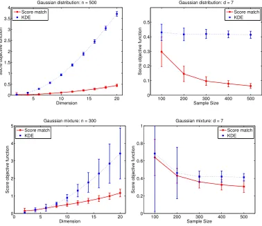
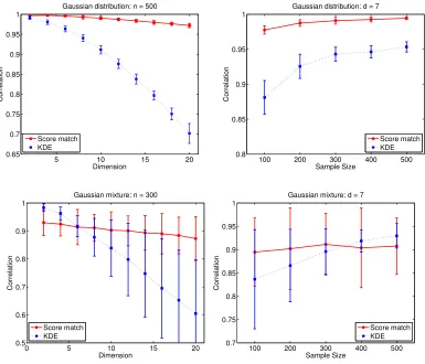
also investigate the misspecified case ofp0∈ P/ and show thatJ(p0kpˆn)→infp∈PJ(p0kp) as n→ ∞, and provide a rate for this convergence under a similar smoothness condition as above. Through numerical simulations we demonstrate that the proposed estimator outperforms the non-parametric kernel density estimator, and that the advantage of the proposed estimator grows asdincreases.
c
Keywords: density estimation, exponential family, Fisher divergence, kernel density estimator, maximum likelihood, interpolation space, inverse problem, reproducing kernel Hilbert space, Tikhonov regularization, score matching
1. Introduction
Exponential families are among the most important classes of parametric models studied in statistics, and include many common distributions such as the normal, exponential, gamma, and Poisson. In its “natural form”, the family generated by a probability densityq0 (defined over Ω⊆Rd) andsufficient statistic,T : Ω→
Rm is defined as
Pfin:=
n
pθ(x) =q0(x)eθTT(x)−A(θ), x∈Ω : θ∈Θ⊂Rm o
(1)
where A(θ) := logR
Ωe
θTT(x)
q0(x)dx is the cumulant generating function (also called the log-partition function), Θ⊂ {θ∈Rm :A(θ)<∞}is thenatural parameter space andθis a
finite-dimensional vector called thenatural parameter. Exponential families have a number of properties that make them extremely useful for statistical analysis (seeBrown,1986for more details).
In this paper, we consider an infinite dimensional generalization (Canu and Smola,2005;
Fukumizu,2009) of (1),
P =
n
pf(x) =ef(x)−A(f)q0(x), x∈Ω :f ∈ F o
,
where the function spaceF is defined as
F =
n
f ∈H:eA(f)<∞o, with A(f) := log
Z
Ω
ef(x)q0(x)dx
being the cumulant generating function, and (H,h·,·iH) a reproducing kernel Hilbert space (RKHS) (Aronszajn,1950) with kas its reproducing kernel. While various generalizations are possible for different choices ofF (e.g., an Orlicz space as inPistone and Sempi,1995), the connection ofPto the natural exponential family in (1) is particularly enlightening when
H is an RKHS. This is due to the reproducing property of the kernel,f(x) =hf, k(x,·)iH, through which k(x,·) takes the role of the sufficient statistic. In fact, it can be shown (see Section 3and Example 1for more details) that every Pfin is generated byP induced by a finite dimensional RKHS H, and therefore the family P with H being an infinite dimensional RKHS is a natural infinite dimensional generalization of Pfin. Furthermore, this generalization is particularly interesting as in contrast to Pfin, it can be shown that
P is a rich class of densities (depending on the choice of k and therefore H) that can approximate a broad class of probability densities arbitrarily well (see Propositions1,13and Corollary2). This generalization is not only of theoretical interest, but also has implications for statistical and machine learning applications. For example, in Bayesian non-parametric density estimation, the densities in P are chosen as prior distributions on a collection of probability densities (e.g., see van der Vaart and van Zanten, 2008). P has also found applications in nonparametric hypothesis testing (Gretton et al., 2012; Fukumizu et al.,
covariance operators, which are obtained as the first and second Fr´echet derivatives ofA(f) (seeFukumizu,2009, Section 1.2.3). Recently, the infinite dimensional exponential family,P
has been used to develop a gradient-free adaptive MCMC algorithm based on Hamiltonian Monte Carlo (Strathmann et al., 2015) and also has been used in the context of learning the structure of graphical models (Sun et al.,2015).
Motivated by the richness of the infinite dimensional generalization and its statistical applications, it is of interest to model densities byP, and therefore the goal of this paper is to estimate unknown densities by elements inP when H is an infinite dimensional RKHS. Formally, given i.i.d. random samples (Xa)na=1drawn from an unknown density p0, the goal is to estimate p0 through P. Throughout the paper, we refer to case of p0 ∈ P as
well-specified, in contrast to the misspecified case where p0 ∈ P/ . The setting is useful because
P is a rich class of densities that can approximate a broad class of probability densities arbitrarily well, hence it may be widely used in place of non-parametric density estimation methods (e.g., kernel density estimation (KDE)). In fact, through numerical simulations, we show in Section 6 that estimating p0 through P performs better than KDE, and that the advantage of the proposed estimator grows with increasing dimensionality.
In the finite-dimensional case where θ ∈ Θ ⊂ Rm, estimating pθ through maximum
likelihood (ML) leads to solving elegant likelihood equations (Brown, 1986, Chapter 5). However, in the infinite dimensional case (assuming p0 ∈ P), as in many non-parametric estimation methods, a straightforward extension of maximum likelihood estimation (MLE) suffers from the problem of ill-posedness (Fukumizu,2009, Section 1.3.1). To address this problem,Fukumizu(2009) proposed a method of sieves involving pseudo-MLE by restricting the infinite dimensional manifold P to a series of finite-dimensional submanifolds, which enlarge as the sample size increases, i.e.,pfˆ(l) is the density estimator with
ˆ
f(l)= arg max
f∈F(l)
1
n n X
a=1
f(Xa)−A(f), (2)
where F(l) = {f ∈ H(l) : eA(f) < ∞} and (H(l))∞
l=1 is a sequence of finite-dimensional subspaces ofHsuch thatH(l)⊂H(l+1)for alll∈
N. While the consistency ofpfˆ(l) is proved
in Kullback-Leibler (KL) divergence (Fukumizu,2009, Theorem 6), the method suffers from many drawbacks that are both theoretical and computational in nature. On the theoretical front, the consistency in Fukumizu (2009, Theorem 6) is established by assuming a decay rate on the eigenvalues of the covariance operator (see (A-2) and the discussion in Section 1.4 ofFukumizu(2009) for details), which is usually difficult to check in practice. Moreover, it is not clear which classes of RKHS should be used to obtain a consistent estimator (Fukumizu,
2009, (A-1)) and the paper does not provide any discussion about the convergence rates. On the practical side, the estimator is not attractive as it can be quite difficult to construct the sequence (H(l))∞l=1 that satisfies the assumptions in Fukumizu (2009, Theorem 6). In fact, the impracticality of the estimator, ˆf(l) is accentuated by the difficulty in efficiently handlingA(f) (though it can be approximated by numerical integration).
Fukumizu(2009), Barron and Sheu proposed the ML estimator pfmˆ , where
ˆ
fm= arg max
f∈Fm
1
n n X
a=1
f(Xa)−A(f)
and Fm is the linear space of dimension m spanned by the chosen basis functions. Under the assumption that logp0 has square-integrable derivatives up to orderr, they showed that
KL(p0kpfmˆ ) =Op0(n
−2r/(2r+1)) withm=n1/(2r+1) for each of the approximating families, where KL(pkq) =Rp(x) log(p(x)/q(x))dx is the KL divergence between p and q. Similar work was carried out by Gu and Qiu (1993), who assumed that logp0 lies in an RKHS, and proposed an estimator based on penalized MLE, with consistency and rates established in Jensen-Shannon divergence. Though these results are theoretically interesting, these estimators are obtained via a procedure similar to that in Fukumizu(2009), and therefore suffers from the practical drawbacks discussed above.
The discussion so far shows that the MLE approach to learning p0 ∈ P results in estimators that are of limited practical interest. To alleviate this, one can treat the problem of estimating p0 ∈ P in a completely non-parametric fashion by using KDE, which is well-studied (Tsybakov, 2009, Chapter 1) and easy to implement. This approach ignores the structure of P, however, and is known to perform poorly for moderate to large d
(Wasserman,2006, Section 6.5) (see also Section 6 of this paper).
1.1 Score Matching and Fisher Divergence
To counter the disadvantages of KDE and pseudo/penalized-MLE, in this paper, we propose to use the score matching method introduced by Hyv¨arinen (2005, 2007). While MLE is based on minimizing the KL divergence, the score matching method involves minimizing the Fisher divergence (also called the Fisher information distance; see Definition 1.13 in
Johnson(2004)) between two continuously differentiable densities, p and q on an open set Ω⊆Rd, given as
J(pkq) = 1 2
Z
Ω
p(x)k∇logp(x)− ∇logq(x)k22 dx, (3)
where ∇logp(x) = (∂1logp(x), . . . , ∂dlogp(x)) with ∂ilogp(x) := ∂xi∂ logp(x). Fisher
di-vergence is closely related to the KL didi-vergence through de Bruijn’s identity (Johnson,2004, Appendix C) and it can be shown thatKL(pkq) =R∞
0 J(ptkqt)dt,wherept=p∗N(0, tId),
qt = q∗N(0, tId), ∗ denotes the convolution, and N(0, tId) denotes a normal distribution
onRdwith mean zero and diagonal covariance witht >0 (see PropositionB.1for a precise
statement; also see Theorem 1 in Lyu,2009). Moreover, convergence in Fisher divergence is a stronger form of convergence than that in KL, total variation and Hellinger distances (see Lemmas E.2 & E.3 in Johnson,2004and Corollary 5.1 in Ley and Swan,2013).
To understand the advantages associated with the score matching method, let us con-sider the problem of density estimation where the data generating distribution (say p0) belongs to Pfin in (1). In other words, given random samples (Xa)na=1 drawn i.i.d. from
MLE approach is well-studied and enjoys nice statistical properties in asymptopia (i.e., asymptotically unbiased, efficient, and normally distributed), the computation of ˆθn can be intractable in many situations as discussed above. In particular, this is the case for
pθ(x) = rAθ((θx)) where rθ ≥0 for all θ∈Θ, A(θ) = R
Ωrθ(x)dx, and the functional form of r is known (as a function of θ and x); yet we do not know how to easily compute A, which is often analytically intractable. In this setting (which is exactly the setting of this paper), assuming pθ to be differentiable (w.r.t. x), and RΩp0(x)k∇logpθ(x)k2
2dx < ∞,∀θ ∈ Θ,
J(p0kpθ) =:J(θ) in (3) reduces to
J(θ) =
d X
i=1
Z
Ω
p0(x)
1
2(∂ilogpθ(x)) 2
+∂i2logpθ(x)
dx+1
2
Z
Ω
p0(x)k∇logp0(x)k22 dx,
(4) through integration by parts (seeHyv¨arinen,2005, Theorem 1), under appropriate regularity conditions onp0andpθfor allθ∈Θ. Here∂i2logpθ(x) := ∂
2
∂x2
i
logpθ(x). The main advantage
of the objective in (3) (and also (4)) is that when it is applied to the situation discussed above where pθ(x) = rAθ((θx)), J(θ) is independent of A(θ), and an estimate of θ0 can be obtained by simply minimizing the empirical counterpart ofJ(θ), given by
Jn(θ) := 1
n n X
a=1
d X
i=1
1
2(∂ilogpθ(Xa)) 2
+∂2i logpθ(Xa)
+1 2
Z
Ω
p0(x)k∇logp0(x)k22 dx.
Since Jn(θ) is also independent of A(θ), ˆθn = arg minθ∈ΘJn(θ) may be easily computable,
unlike the MLE. We would like to highlight that while the score matching approach may have computational advantages over MLE, it only estimatespθup to the scaling factorA(θ), and
therefore requires the approximation or computation ofA(θ) through numerical integration to estimatepθ. Note that this issue (of computingA(θ) through numerical integration) exists even with MLE, but not with KDE. In score matching, however, numerical integration is needed only once, while MLE would typically require a functional form of the log-partition function which is approximated through numerical integration at every step of an iterative optimization algorithm (for example, see (2)), thus leading to major computational savings. An important application that does not require the computation ofA(θ) is in finding modes of the distribution, which has recently become very popular in image processing (Comaniciu and Meer,2002), and has already been investigated in the score matching framework (Sasaki et al.,2014). Similarly, in sampling methods such as sequential Monte Carlo (Doucet et al.,
2001), it is often the case that the evaluation of unnormalized densities is sufficient to calculate required importance weights.
1.2 Contributions
(i) We present an estimate of p0 ∈ P in the well-specified case through the minimization of Fisher divergence, in Section4. First, we show that estimatingp0 :=pf0 using the score
matches the MLE (Hyv¨arinen, 2005). The estimator obtained in the infinite dimensional case is not a simple extension of its finite-dimensional counterpart, however, as the former requires an appropriate regularizer (we use k · k2
H) to make the problem well-posed. We would like to highlight that to the best of our knowledge, the proposed estimator is the first practically computable estimator ofp0 with consistency guarantees (see below).
(ii)In contrast toHyv¨arinen(2007) where no guarantees on consistency or convergence rates are provided for the density estimator in Pfin, we establish in Theorem6 the consistency and rates of convergence for the proposed estimator off0, and use these to prove consistency and rates of convergence for the corresponding plug-in estimator ofp0(Theorems7andB.2), even whenH is infinite dimensional. Furthermore, while the estimator off0 (and therefore
p0) is obtained by minimizing the Fisher divergence, the resultant density estimator is also shown to be consistent in KL divergence (and therefore in Hellinger and total-variation distances) and we provide convergence rates in all these distances.
Formally, we show that the proposed estimator ˆfn is converges as
kf0−fˆnkH=Op0(n
−α), KL(p
0kpfnˆ ) =Op0(n
−2α) and J(p
0kpfnˆ ) =Op0
n−min
n
2 3,
2β+1 2β+2
o
if f0 ∈ R(Cβ) for some β > 0, where R(A) denotes the range or image of an operator
A, α = min{14,2ββ+2}, and C := Pdi=1RΩ∂ik(x,·)⊗∂ik(x,·)p0(x)dx is a Hilbert-Schmidt operator on H (see Theorem 4) with k being the reproducing kernel and ⊗ denoting the tensor product. When H is a finite-dimensional RKHS, we show that the estimator enjoys parametric rates of convergence, i.e.,
kf0−fnˆkH=Op0(n
−1/2), KL(p
0kpfnˆ ) =Op0(n
−1
) andJ(p0kpfnˆ) =Op0(n
−1 ).
Note that the convergence rates are obtained under a non-classical smoothness assumption on f0, namely that it lies in the image of certain fractional power of C, which reduces to a more classical assumption if we choose k to be a Mat´ern kernel (see Section 2 for its definition), as it induces a Sobolev space. In Section4.2, we discuss in detail the smoothness assumption onf0 for the Gaussian (Example2) and Mat´ern (Example3) kernels. Another interesting point to observe is that unlike in the classical function estimation methods (e.g., kernel density estimation and regression), the rates presented above for the proposed estimator tend to saturate forβ >1 (β > 12 w.r.t. J), with the best rate attained atβ = 1 (β = 12 w.r.t.J), which means the smoothness off0 is not fully captured by the estimator. Such a saturation behavior is well-studied in the inverse problem literature (Engl et al.,
1996) where it has been attributed to the choice of regularizer. In Section4.3, we discuss alternative regularization strategies using ideas fromBauer et al.(2007), which covers non-parametric least squares regression: we show that for appropriately chosen regularizers, the above mentioned rates hold for any β > 0, and do not saturate for the aforementioned ranges of β (see Theorem9).
(iii) In Section 5, we study the problem of density estimation in the misspecified setting, i.e., p0 ∈ P/ , which is not addressed in Hyv¨arinen (2007) and Fukumizu (2009). Using a more sophisticated analysis than in the well-specified case, we show in Theorem 12 that
on logp0
q0 (see the statement of Theorem 12 for details), we show that J(p0kpfnˆ ) → 0 as
n → ∞ along with a rate for this convergence, even though p0 ∈ P/ . However, unlike in the well-specified case, where the consistency is obtained not only in J but also in other distances, we obtain convergence only inJ for the misspecified case. Note that whileBarron and Sheu (1991) considered the estimation ofp0 in the misspecified setting, the results are restricted to the approximating families consisting of polynomials, splines, or trigonometric series. Our results are more general, as they hold for abstract RKHSs.
(iv)In Section6, we present preliminary numerical results comparing the proposed estimator with KDE in estimating a Gaussian and mixture of Gaussians, with the goal of empirically evaluating performance as d gets large for a fixed sample size. In these two estimation problems, we show that the proposed estimator outperforms KDE, and the advantage grows asdincreases. Inspired by this preliminary empirical investigation, our proposed estimator (or computationally efficient approximations) has been used by Strathmann et al. (2015) in a gradient-free adaptive MCMC sampler, and by Sun et al. (2015) for graphical model structure learning. These applications demonstrate the practicality and performance of the proposed estimator.
Finally, we would like to make clear that our principal goal is not to construct density estimators that improve uniformly upon KDE, but to provide a novel flexible modeling technique for approximating an unknown density by a rich parametric family of densities, with the parameter being infinite dimensional, in contrast to the classical approach of finite dimensional approximation.
Various notations and definitions that are used throughout the paper are collected in Section2. The proofs of the results are provided in Section 8, along with some supplemen-tary results in an appendix.
2. Definitions & Notation
We introduce the notation used throughout the paper. Define [d] :={1, . . . , d}. For a :=
(a1, . . . , ad)∈Rdandb:= (b1, . . . , bd)∈Rd,kak2 :=
q Pd
i=1a2i andha, bi:= Pd
i=1aibi. For
a, b >0, we write a.b ifa≤γb for some positive universal constant γ. For a topological spaceX,C(X) (resp. Cb(X)) denotes the space of all continuous (resp. bounded continuous)
functions on X. For a locally compact Hausdorff space X, f ∈ C(X) is said to vanish at infinity if for every >0 the set{x:|f(x)| ≥} is compact. The class of all continuousf
on X which vanish at infinity is denoted as C0(X). For open X ⊂Rd,C1(X) denotes the
space of continuously differentiable functions onX. Forf ∈Cb(X), kfk∞:= supx∈X|f(x)| denotes the supremum norm of f. Mb(X) denotes the set of all finite Borel measures on X. For µ ∈ Mb(X), Lr(X, µ) denotes the Banach space of r-power (r ≥ 1) µ-integrable
functions. For X ⊂ Rd, we will use Lr(X) for Lr(X, µ) if µ is a Lebesgue measure onX.
For f ∈ Lp(X, µ), kfkLr(X,µ) := RX|f|rdµ1/r denotes the Lr-norm of f for 1 ≤ r < ∞
and we denote it as k · kLr(X) ifX ⊂ Rd and µ is the Lebesgue measure. The convolution f∗g of two measurable functions f and g onRd is defined as
(f∗g)(x) :=
Z
Rd
provided the integral exists for all x∈Rd. The Fourier transform of f ∈L1(
Rd) is defined
as
f∧(y) = (2π)−d/2
Z
Rd
f(x)e−ihy,xidx
whereidenotes the imaginary unit √−1.
In the following, for the sake of completeness and simplicity, we present definitions restricted to Hilbert spaces. LetH1 andH2be abstract Hilbert spaces. A mapS:H1→H2 is called alinear operator if it satisfiesS(αx) =αSxandS(x+x0) =Sx+Sx0 for allα∈R
andx, x0 ∈H1, whereSx:=S(x). A linear operatorS is said to bebounded, i.e., the image
SBH1 ofBH1 underS is bounded if and only if there exists a constantc∈[0,∞) such that
for allx∈H1 we havekSxkH2 ≤ckxkH1, whereBH1 :={x∈H1 :kxkH1 ≤1}. In this case,
theoperator norm ofS is defined askSk:= sup{kSxkH2 :x∈BH1}. DefineL(H1, H2) be
the space of bounded linear operators fromH1 toH2. S ∈ L(H1, H2) is said to becompact ifSBH1 is a compact subset inH2. The adjoint operator S
∗ :H
2 → H1 of S ∈ L(H1, H2) is defined by hx, S∗yi
H1 = hSx, yiH2, x ∈ H1, y ∈ H2. S ∈ L(H) := L(H, H) is called
self-adjoint ifS∗ =S and is calledpositive ifhSx, xiH ≥0 for allx∈H. α∈Ris called an eigenvalueofS ∈ L(H) if there exists anx6= 0 such thatSx=αxand such anxis called the
eigenvector ofSand α. For compact, positive, self-adjointS∈ L(H),Sr :H→H,r ≥0 is called afractional power ofSandS1/2is thesquare root ofS, which we write as√S :=S1/2. An operator S ∈ L(H1, H2) isHilbert-Schmidt ifkSkHS := (Pj∈JkSejk2H2)
1/2 <∞ where (ej)j∈J is an arbitrary orthonormal basis of separable Hilbert space H1. S ∈ L(H1, H2) is said to be of trace class ifP
j∈Jh(S∗S)1/2ej, ejiH1 <∞. Forx ∈H1 and y∈ H2, x⊗y is
an element of the tensor product spaceH1⊗H2 which can also be seen as an operator from
H2 toH1 as (x⊗y)z=xhy, ziH2 for anyz∈H2. R(S) denotes therange space (or image)
of S.
A real-valued symmetric functionk:X × X →Ris called a positive definite (pd) kernel
if, for all n∈N,α1, . . . , αn ∈Rand all x1, . . . , xn ∈ X, we have Pni,j=1αiαjk(xi, xj)≥0. A function k : X × X → R,(x, y) 7→ k(x, y) is a reproducing kernel of the Hilbert space (Hk,h·,·iHk) of functions if and only if (i) ∀y ∈ X, k(y,·) ∈ Hk and (ii) ∀y ∈ X, ∀f ∈ Hk, hf, k(y,·)iHk = f(y) hold. If such a k exists, then Hk is called a reproducing kernel Hilbert space. Since hk(x,·), k(y,·)iHk = k(x, y),∀x, y ∈ X, it is easy to show that every
reproducing kernel (r.k.) k is symmetric and positive definite. Some examples of kernels that appear throughout the paper are: Gaussian kernel,k(x, y) = exp(−σkx−yk2
2), x, y∈
Rd, σ >0 that induces the followingGaussian RKHS,
Hk =Hσ :=nf ∈L2(Rd)∩C(Rd) : Z
|f∧(ω)|2ekωk22/4σdω <∞
o ,
theinverse multiquadric kernel,k(x, y) = (1 +kx−cyk2
2)−β, x, y∈Rd, β >0, c∈(0,∞) and the Mat´ern kernel, k(x, y) = 2Γ(1−ββ)kx−yk2β−d/2Kd/2−β(kx−yk2), x, y ∈ Rd, β > d/2 that
induces the Sobolev space, H2β,
Hk=H2β :=
n
f ∈L2(Rd)∩C(Rd) : Z
(1 +kωk22)β|f∧(ω)|2dω <∞o,
where Γ is the Gamma function, and Kv is the modified Bessel function of the third kind
For any real-valued function f defined on open X ⊂ Rd, f is said to be m-times
con-tinuously differentiable if for α∈Nd0 with|α|:=
Pd
i=1αi ≤m,∂αf(x) =∂
α1
1 . . . ∂
αd
d f(x) = ∂|α|
∂xα1 1 ...∂xαdd
f(x) exists. A kernel k is said to be m-times continuously differentiable if
∂α,αk : X × X → R exists and is continuous for all α ∈ Nd
0 with |α| ≤ m where ∂α,α :=
∂α1
1 . . . ∂
αd
d ∂
α1
1+d. . . ∂ αd
2d. Corollary 4.36 inSteinwart and Christmann(2008) and Theorem 1
inZhou(2008) state that if∂α,αkexists and is continuous, then∂αk(x,·) =∂α1
1 . . . ∂
αd d k(x,·)
= ∂|α|
∂xα1 1 ...∂xαdd
k((x1, . . . , xd),·) ∈ Hk with x = (x1, . . . , xd) and for every f ∈ Hk, we have ∂αf(x) =h∂αk(x,·), fi
Hk and ∂
α,αk(x, x0) =h∂αk(x,·), ∂αk(x0,·)i Hk.
Given two probability densities, p and q on Ω ⊂ Rd, the Kullback-Leibler divergence
(KL) and Hellinger distance (h) are defined asKL(pkq) = R p(x) logpq((xx))dx and h(p, q) =
k√p−√qkL2(Ω) respectively. We refer tokp−qkL1(Ω) as the total variation (TV) distance
betweenp and q.
3. Approximation of Densities by P
In this section, we first show that every finite dimensional exponential family, Pfin is gen-erated by the familyP induced by a finite dimensional RKHS, which naturally leads to the infinite dimensional generalization of Pfin when H is an infinite dimensional RKHS. Next, we investigate the approximation properties ofP in Proposition 1and Corollary 2whenH is an infinite dimensional RKHS.
Let us consider a r-parameter exponential family, Pfin with sufficient statisticT(x) := (T1(x), . . . , Tr(x)) and construct a Hilbert space,H= span{T1(x), . . . , Tr(x)}. It is easy to
verify thatP induced by H is exactly the same as Pfin since any f ∈H can be written as
f(x) = Pri=1θiTi(x) for some (θi)ri=1 ⊂R. In fact, by defining the inner product between
f = Pri=1θiTi and g = Pri=1γiTi as hf, giH := Pri=1θiγi, it follows that H is an RKHS
with the r.k. k(x, y) = hT(x), T(y)iRr sincehf, k(x,·)iH =Pr
i=1θiTi(x) = f(x). Based on this equivalence betweenPfin and P induced by a finite dimensional RKHS, it is therefore clear thatP induced by a infinite dimensional RKHS is a strict generalization toPfin with
k(·, x) playing the role of a sufficient statistic.
Example 1 The following are some popular examples of probability distributions that be-long to Pfin. Here we show the corresponding RKHSs (H, k) that generate these
distribu-tions. In some of these examples, we choose q0(x) = 1 and ignore the fact that q0 is a
probability distribution as assumed in the definition of P.
Exponential:Ω =R++:=R+\{0}, k(x, y) =xy.
Normal: Ω =R,k(x, y) =xy+x2y2.
Beta: Ω = (0,1),k(x, y) = logxlogy+ log(1−x) log(1−y).
Gamma: Ω =R++, k(x, y) = logxlogy+xy.
Inverse Gaussian: Ω =R++, k(x, y) =xy+xy1 .
Binomial: Ω ={0, . . . , m}, k(x, y) =xy, q0(x) = 2−m mc
.
While Example 1shows that all popular probability distributions are contained inP for an appropriate choice of finite-dimensionalH, it is of interest to understand the richness of
P (i.e., what class of distributions can be approximated arbitrarily well by P?) whenH is an infinite dimensional RKHS. This is addressed by the following result, which is proved in Section8.1.
Proposition 1 Define
P0 :=nπf(x) =ef(x)−A(f)q0(x), x∈Ω :f ∈C0(Ω)
o
where Ω⊆Rd is locally compact Hausdorff. Suppose k(x,·)∈C
0(Ω),∀x∈Ω and
Z Z
k(x, y)dµ(x)dµ(y)>0, ∀µ∈Mb(Ω)\{0}. (5)
Then P is dense in P0 w.r.t. Kullback-Leibler divergence, total variation (L1 norm) and Hellinger distances. In addition, if q0∈L1(Ω)∩Lr(Ω)for some1< r≤ ∞, then P is also
dense in P0 w.r.t. Lr norm.
A sufficient condition for Ω⊆Rd to be locally compact Hausdorff is that it is either open
or closed. Condition (5) is equivalent to k beingc0-universal (Sriperumbudur et al., 2011, p. 2396). If k(x, y) = ψ(x−y), x, y ∈ Ω = Rd where ψ ∈ Cb(Rd)∩L1(Rd), then (5)
can be shown to be equivalent to supp(ψ∧) =Rd (Sriperumbudur et al.,2011, Proposition
5). Examples of kernels that satisfy the conditions in Proposition 1 include the Gaussian, Mat´ern and inverse multiquadrics. In fact, any compactly supported non-zeroψ∈Cb(Rd)
satisfies the assumptions in Proposition 1 as supp(ψ∧) =Rd (Sriperumbudur et al., 2010,
Corollary 10). ThoughP0 is still a parametric family of densities indexed by a Banach space (here C0(Ω)), the following corollary (proved in Section8.2) to Proposition 1shows that a broad class of continuous densities are contained in P0 and therefore can be approximated arbitrarily well inLr norm (1≤r≤ ∞), Hellinger distance, and KL divergence byP.
Corollary 2 Let q0 ∈ C(Ω) be a probability density such that q0(x) > 0 for all x ∈ Ω,
where Ω⊆Rd is locally compact Hausdorff. Suppose there exists a constant` such that for any >0, ∃R >0 that satisfies |qp(x)
0(x) −`| ≤ for anyx with kxk2> R. Define
Pc:=
p∈C(Ω) :
Z
Ω
p(x)dx= 1, p(x)≥0,∀x∈Ω and p
q0
−`∈C0(Ω)
.
Supposek(x,·)∈C0(Ω),∀x∈Ωand (5) holds. ThenP is dense inPcw.r.t. KL divergence, TV and Hellinger distances. Moreover, ifq0∈L1(Ω)∩Lr(Ω)for some 1< r≤ ∞, then P
is also dense in Pc w.r.t. Lr norm.
Similar to the results so far, an approximation result for P can also be obtained w.r.t. Fisher divergence (see Proposition 13). Since this result is heavily based on the notions and results developed in Section 5, we defer its presentation until that section. Briefly, this result states that if H is sufficiently rich (i.e., dense in an appropriate class of functions), then any p∈C1(Ω) withJ(pkq0)<∞ can be approximated arbitrarily well by elements inP w.r.t. Fisher divergence, where q0 ∈C1(Ω).
4. Density Estimation in P: Well-specified Case
In this section, we present our score matching estimator for an unknown densityp0:=pf0 ∈
P (well-specified case) from i.i.d. random samples (Xa)na=1 drawn from it. This involves choosing the minimizer of the (empirical) Fisher divergence between p0 and pf ∈ P as the estimator, ˆf which we show in Theorem 5 to be obtained by solving a simple finite-dimensional linear system. In contrast, we would like to remind the reader that the MLE is infeasible in practice due to the difficulty in handlingA(f). The consistency and convergence rates of ˆf ∈ F and the plug-in estimator pfˆ are provided in Section 4.1 (see Theorems 6 and 7). Before we proceed, we list the assumptions on p0, q0 and H that we need in our analysis.
(A) Ω is a non-empty open subset of Rd with a piecewise smooth boundary∂Ω := Ω\Ω,
where Ω denotes the closure of Ω.
(B) p0 is continuously extendible to Ω. k is twice continuously differentiable on Ω×Ω with continuous extension of∂α,αk to Ω×Ω for|α| ≤2.
(C) ∂i∂i+dk(x, x)p0(x) = 0 for x ∈ ∂Ω and
p
∂i∂i+dk(x, x)p0(x) = o(kxk1−2 d) as x ∈ Ω,
kxk2→ ∞ for all i∈[d].
(D) (ε-Integrability) For some ε ≥ 1 and ∀i ∈ [d], ∂i∂i+dk(x, x),
q
∂2i∂i2+dk(x, x) and
p
∂i∂i+dk(x, x)∂ilogq0(x)∈Lε(Ω, p0),whereq0 ∈C1(Ω).
Remark 3 (i) Ω being a subset of Rd along with k being continuous ensures that H is separable (Steinwart and Christmann, 2008, Lemma 4.33). The twice differentiability of k ensures that every f ∈ H is twice continuously differentiable (Steinwart and Christmann, 2008, Corollary 4.36). (C) ensures that J in (3) is equivalent to the one in (4) through integration by parts on Ω (see Corollary 7.6.2 in Duistermaat and Kolk, 2004 for inte-gration by parts on bounded subsets of Rd which can be extended to unbounded Ω through a truncation and limiting argument) for densities in P. In particular, (C) ensures that R
Ω∂if(x)∂ip0(x)dx=−
R
Ω∂ 2
if(x)p0(x)dxfor allf ∈Handi∈[d], which will be critical to
prove the representation in Theorem 4(ii), upon which rest of the results depend. The decay condition in (C)can be weakened top∂i∂i+dk(x, x)p0(x) =o(kxk1−2 d)asx∈Ω,kxk2 → ∞
for alli∈[d]if Ω is a (possibly unbounded) box where d= #{i∈[d]|(ai, bi) is unbounded}.
(ii) When ε = 1, the first condition in (D) ensures that J(p0kpf) < ∞ for any pf ∈ P. The other two conditions ensure the validity of the alternate representation for J(p0kpf)
kernels that satisfy (D) are the Gaussian, Mat´ern (with β > max{2, d/2}), and inverse multiquadric kernels, for which it is easy to show that there exists q0 that satisfies (D). (iii) (Identifiability) The above list of assumptions do not include the identifiability condi-tion that ensures pf1 =pf2 if and only if f1 =f2. It is clear that if constant functions are
included in H, i.e., 1 ∈ H, then pf = pf+c for any c ∈ R. On the other hand, it can be shown that if 1∈/ H and supp(q0) = Ω, then pf1 =pf2 ⇔ f1 =f2. A sufficient condition
for 1 ∈/ H is k∈C0(Ω×Ω). We do not explicitly impose the identifiability condition as a
part of our blanket assumptions because the assumptions under which consistency and rates are obtained in Theorem 7 automatically ensure identifiability.
Under these assumptions, the following result—proved in Section8.3—shows that the prob-lem of estimating p0 through the minimization of Fisher divergence reduces to the problem of estimatingf0 through a weighted least squares minimization inH(see parts (i) and (ii)). This motivates the minimization of the regularized empirical weighted least squares (see part (iv)) to obtain an estimator fλ,n of f0, which is then used to construct the plug-in estimate pfλ,n ofp0.
Theorem 4 Suppose (A)–(D) hold with ε= 1. Then J(p0kpf) < ∞ for all f ∈ F. In addition, the following hold.
(i) For all f ∈ F,
J(f) :=J(p0kpf) = 1
2hf−f0, C(f −f0)iH, (6)
where C : H → H, C := RΩp0(x)Pdi=1∂ik(x,·) ⊗∂ik(x,·)dx is a trace-class positive operator with
Cf =
Z
Ω
p0(x)
d X
i=1
∂ik(x,·)∂if(x)dx.
(ii) Alternatively,
J(f) = 1
2hf, CfiH+hf, ξiH+J(p0kq0)
where
ξ:=
Z
Ω
p0(x)
d X
i=1
∂ik(x,·)∂ilogq0(x) +∂i2k(x,·)
dx∈H
and f0 satisfiesCf0 =−ξ.
(iii) For any λ >0, a unique minimizer fλ of Jλ(f) :=J(f) +λ2kfk2
H over H exists and is
given by
fλ =−(C+λI)−1ξ = (C+λI)−1Cf0.
(iv) (Estimator of f0) Given samples (Xa)na=1 drawn i.i.d. from p0, for any λ > 0, the
where Jˆ(f) := 12hf,Cfiˆ H+hf,ξiˆH+J(p0kq0), Cˆ := 1nPna=1
Pd
i=1∂ik(Xa,·)⊗∂ik(Xa,·) and
ˆ
ξ := 1
n n X
a=1
d X
i=1
∂ik(Xa,·)∂ilogq0(Xa) +∂i2k(Xa,·)
.
An advantage of the alternate formulation of J(f) in Theorem 4(ii) over (6) is that it provides a simple way to obtain an empirical estimate of J(f)—by replacing C and ξ by their empirical estimators, ˆC and ˆξ respectively—from finite samples drawn i.i.d. from p0, which is then used to obtain an estimator of f0. Note that the empirical estimate ofJ(f), i.e., ˆJ(f) depends only on ˆC and ˆξ which in turn depend on the known quantities, k and
q0, and therefore fλ,n in Theorem 4(iv) should in principle be computable. In practice,
however, it is not easy to compute the expression for fλ,n = −( ˆC+λI)−1ξˆas it involves
solving an infinite dimensional linear system. In Theorem 5 (proved in Section 8.4), we provide an alternative expression forfλ,nas a solution of a simple finite-dimensional linear
system (see (7) and (8)), using the general representer theorem (see Theorem A.2). It is interesting to note that while the solution to J(f) in Theorem 4(ii) is obtained by solving a non-linear system,Cf0 =−ξ (the system is non-linear asC depends on p0 which in turn depends on f0), its estimator fλ,n proposed in Theorem 4, is obtained by solving a simple
linear system. In addition, we would like to highlight the fact that the proposed estimator,
fλ,n is precisely the Tikhonov regularized solution (which is well-studied in the theory of
linear inverse problems) to the ill-posed linear system ˆCf = −ξˆ. We further discuss the choice of regularizer in Section 4.3using ideas from the inverse problem literature.
An important remark we would like to make about Theorem 4 is that though J(f) in (6) is valid only forf ∈ F, as it is obtained fromJ(p0kpf) where p0, pf ∈ P, the expression hf −f0, C(f −f0)iH is valid for any f ∈H, as it is finite under the assumption that (D) holds withε= 1. Therefore, in Theorem 4(iii, iv), fλ and fλ,nare obtained by minimizing
Jλ and ˆJλ overH instead of overF, as the latter does not yield a nice expression (unlike
fλ andfλ,n, respectively). However, there is no guarantee that fλ,n∈ F, and so the density
estimatorpfλ,n may not be valid. While this is not an issue when studying the convergence
ofkfλ,n−f0kH(see Theorem6), the convergence ofpfλ,n top0 (in various distances) needs
to be handled slightly differently depending on whether the kernel is bounded or not (see Theorems 7 and B.2). Note that when the kernel is bounded, we obtain F = H, which implies pfλ,n is valid.
Theorem 5 (Computation of fλ,n) Let fλ,n= arg inff∈HJˆλ(f), where Jˆλ(f) is defined in Theorem 4(iv) and λ >0. Then
fλ,n=−ξˆ
λ+
n X
a=1
d X
i=1
β(a−1)d+i∂ik(Xa,·), (7)
where ξˆis defined in Theorem 4(iv) and β= (β(a−1)d+i)a,i is obtained by solving
(G+nλI)β= 1
with (G)(a−1)d+i,(b−1)d+j =∂i∂j+dk(Xa, Xb) and
(h)(a−1)d+i =hξ, ∂ikˆ (Xa,·)iH=
1
n n X
b=1
d X
j=1
∂i∂j2+dk(Xa, Xb) +∂i∂j+dk(Xa, Xb)∂jlogq0(Xb).
We would like to highlight that thoughfλ,n requires solving a simple linear system in (8),
it can still be computationally intensive whend andn are large as Gis and×nd matrix. This is still a better scenario than that of MLE, however, since computationally efficient methods exist to solve large linear systems such as (8), whereas MLE can be intractable due to the difficulty in handling the log-partition function (though it can be approximated). On the other hand, MLE is statistically well-understood, with consistency and convergence rates established in general for the problem of density estimation (van de Geer,2000) and in particular for the problem at hand (Fukumizu, 2009). In order to ensure that fλ,n and pfλ,n are statistically useful, in the following section, we investigate their consistency and convergence rates under some smoothness conditions onf0.
4.1 Consistency and Rate of Convergence
In this section, we prove the consistency offλ,n(see Theorem6(i)) andpfλ,n(see Theorems7
and B.2). Under the smoothness assumption that f0 ∈ R(Cβ) for some β >0, we present convergence rates for fλ,n and pfλ,n in Theorems 6(ii), 7 and B.2. In reference to the
following results, for simplicity we suppress the dependence of λ on nby defining λ:=λn
where (λn)n∈N⊂(0,∞).
Theorem 6 (Consistency and convergence rates for fλ,n) Suppose(A)–(D)withε= 2 hold.
(i) Iff0 ∈ R(C), then kfλ,n−f0kH
p0
→0 asλ→0, λ√n→ ∞ andn→ ∞.
(ii) Iff0 ∈ R(Cβ) for some β >0, then for λ=n −max
n
1 4,
1 2(β+1)
o ,
kfλ,n−f0kH=Op0
n−min
n
1 4,
β
2(β+1)
o
as n→ ∞.
(iii) IfkC−1k<∞, then forλ=n−12, kfλ,n−f0kH=Op 0(n
−1/2) as n→ ∞.
Remark (i) While Theorem6(proved in Section8.5) provides an asymptotic behavior for
kfλ,n−f0kH under conditions that depend on p0 (and are therefore not easy to check in practice), a non-asymptotic bound onkfλ,n−f0kHthat holds for alln≥1 can be obtained under stronger assumptions through an application of Bernstein’s inequality in separable Hilbert spaces. For the sake of simplicity, we provided asymptotic results which are obtained through an application of Chebyshev’s inequality.
(ii) The proof of Theorem 6(i) involves decomposing kfλ,n−f0kH into an estimation error part,E(λ, n) :=kfλ,n−fλkH, and an approximation error part,A0(λ) :=kfλ−f0kH, where
A0(λ) → 0 as λ → 0 without assuming f0 ∈ R(C). This is because, if f0 lies in the null space ofC, then fλ is zero irrespective of λand therefore cannot approximate f0.
(iii) The condition f0 ∈ R(C) is difficult to check in practice as it depends on p0 (which in turn depends onf0). However, since the null space ofC is just constant functions if the kernel is bounded and supp(q0) = Ω (see Lemma 14 in Section 8.6 for details), assuming 1 ∈/ H yields that R(C) = H and therefore consistency can be attained under conditions that are easy to impose in practice. As mentioned in Remark 3(iii), the condition 1 ∈/ H
ensures identifiability and a sufficient condition for it to hold is k ∈ C0(Ω×Ω), which is satisfied by Gaussian, Mat´ern and inverse multiquadric kernels.
(iv)It is well known that convergence rates are possible only if the quantity of interest (here
f0) satisfies some additional conditions. In function estimation, this additional condition is classically imposed by assumingf0 to be sufficiently smooth, e.g.,f0 lies in a Sobolev space of certain smoothness. By contrast, the smoothness condition in Theorem6(ii) is imposed in an indirect manner by assuming f0 ∈ R(Cβ) for some β > 0—so that the results hold for abstract RKHSs and not just Sobolev spaces—which then provides a rate, with the best rate being n−1/4 that is attained when β ≥ 1. While such a condition has already been used in various works (Caponnetto and Vito,2007;Smale and Zhou,2007;Fukumizu et al.,2013) in the context of non-parametric least squares regression, we explore it in more detail in Proposition8, and Examples 2 and 3. Note that this condition is common in the inverse problem theory (seeEngl, Hanke, and Neubauer,1996), and it naturally arises here through the connection offλ,nbeing a Tikhonov regularized solution to the ill-posed linear
system ˆCf = −ξˆ. An interesting observation about the rate is that it does not improve with increasingβ(forβ >1), in contrast to the classical results in function estimation (e.g., kernel density estimation and kernel regression) where the rate improves with increasing smoothness. This issue is discussed in detail in Section 4.3.
(v)SincekC−1k<∞only ifHis finite-dimensional, we recover the parametric rate ofn−1/2
in a finite-dimensional situation with an automatic choice for λasn−1/2.While Theorem 6
provides statistical guarantees for parameter convergence, the question of primary interest is the convergence ofpfλ,n top0. This is guaranteed by the following result, which is proved
in Section8.6.
Theorem 7 (Consistency and rates for pfλ,n) Suppose (A)–(D) with ε = 2 hold and kkk∞:= supx∈Ωk(x, x)<∞. Assume supp(q0) = Ω. Then the following hold:
(i) For any 1< r≤ ∞with q0 ∈L1(Ω)∩Lr(Ω),
kpfλ,n−p0kLr(Ω)→0, h(pfλ,n, p0)→0, KL(p0kpfλ,n)→0 as λ √
n→ ∞, λ→0and n→ ∞.
In addition, if f0 ∈ R(Cβ) for some β >0, then for λ=n −max
n
1 4,
1 2(β+1)
o ,
kpfλ,n−p0kLr(Ω)=Op0(θn), h(p0, pf
λ,n) =Op0(θn), KL(p0kpfλ,n) =Op0(θ
2
n)
as n→ ∞ where θn:=n
−min
n
1 4,
β
2(β+1)
o .
β ≥0, then for λ=n−max n
1 3,
1 2(β+1)
o ,
J(p0kpfλ,n) =Op0
n−min
n
2 3,
2β+1 2(β+1)
o
as n→ ∞.
(iii) IfkC−1k<∞, then θn=n−12 and J(p0kpfλ,n) =Op 0(n
−1) withλ=n−1 2.
Remark (i) Comparing the results of Theorem 6(i) and Theorem 7(i) (for Lr, Hellinger and KL divergence), we would like to highlight that while the conditions onλandnmatch in both the cases, the latter does not require f0 ∈ R(C) to ensure consistency. While
f0 ∈ R(C) can be imposed in Theorem 7 to attain consistency, we replaced this condition with supp(q0) = Ω—a simple and easy condition to work with—which along with the boundedness of the kernel ensures that for any f0 ∈H, there exists ˜f0 ∈ R(C) such that
pf˜0 =p0 (see Lemma14).
(ii) In contrast to the results in Lr, Hellinger and KL divergence, consistency inJ can be obtained withλ converging to zero at a rate faster than in these results. In addition, one can obtain rates inJ withβ = 0, i.e., no smoothness assumption onf0, while no rates are possible in other distances (the latter might also be an artifact of the proof technique, as these results are obtained through an application of Theorem6(ii) in LemmaA.1) which is due to the fact that the convergence in these other distances is based on the convergence of
kfλ,n−f0kH, which in turn involves convergence of A0(λ) :=kfλ−f0kH to zero while the convergence inJ is controlled byA1
2(λ) :=
k√C(fλ−f0)kH which can be shown to behave
asO(√λ) asλ→0, without requiring any assumptions onf0(see PropositionA.3). Indeed, as a further consequence, the rate of convergence in J is faster than in other distances.
(iii) An interesting aspect in Theorem7 is thatpfλ,n is consistent in various distances such
as Lr, Hellinger and KL, despite being obtained by minimizing a different loss function, i.e., J. However, we will see in Section5 that such nice results are difficult to obtain in the misspecified case, where consistency and rates are provided only in J.
While Theorem 7 addresses the case of bounded kernels, the case of unbounded kernels requires a technical modification. The reason for this modification, as alluded to in the discussion following Theorem 4, is due to the fact that fλ,n may not be in F when k
is unbounded, and therefore the corresponding density estimator, pfλ,n may not be well-defined. In order to keep the main ideas intact, we discuss the unbounded case in detail in SectionB.2 in AppendixB.
4.2 Range Space Assumption
While Theorems 6 and 7 are satisfactory from the point of view of consistency, we believe the presented rates are possibly not minimax optimal since these rates are valid for any RKHS that satisfies the conditions (A)–(D) and does not capture the smoothness of k
(and therefore the corresponding H). In other words, the rates presented in Theorems 6
the intrinsic smoothness of H, they are obtained under the smoothness assumption, i.e.,
range space condition that f0 ∈ R(Cβ) for some β > 0. This condition is quite different from the classical smoothness conditions that appear in non-parametric function estimation. While the range space assumption has been made in various earlier works (e.g.,Caponnetto and Vito (2007); Smale and Zhou (2007); Fukumizu et al. (2013) in the context of non-parametric least square regression), in the following, we investigate the implicit smoothness assumptions that it makes on f0 in our context. To this end, first it is easy to show (see the proof of Proposition B.3in Section B.3) that
R(Cβ) =
( X
i∈I
ciφi : X
i∈I
c2iαi−2β <∞ )
, (9)
where (αi)i∈I are the positive eigenvalues ofC, (φi)i∈I are the corresponding eigenvectors
that form an orthonormal basis for R(C), and I is an index set which is either finite (if
H is finite-dimensional) orI =N with limi→∞αi = 0 (ifH is infinite dimensional). From (9) it is clear that larger the value ofβ, the faster is the decay of the Fourier coefficients (ci)i∈I, which in turn implies that the functions in R(Cβ) are smoother. Using (9), an
interpretation can be provided for R(Cβ) (β >0 and β /∈ N) as interpolation spaces (see
SectionA.5for the definition of interpolation spaces) betweenR(Cdβe) andR(Cbβc) where
R(C0) :=H(see PropositionB.3for details). While it is not completely straightforward to obtain a sufficient condition forf0∈ R(Cβ),β∈N, the following result provides a necessary
condition forf0 ∈ R(C) (and therefore a necessary condition for f0 ∈ R(Cβ),∀β >1) for translation invariant kernels on Ω =Rd, whose proof is presented in Section8.7.
Proposition 8 (Necessary condition) Suppose ψ, φ∈Cb(Rd)∩L1(Rd) are positive def-inite functions on Rd with Fourier transformsψ∧ and φ∧ respectively. Let H and G be the RKHSs associated withk(x, y) =ψ(x−y)andl(x, y) =φ(x−y), x, y∈Rdrespectively. For
1≤r≤2, suppose the following hold:
(i) R
Rdkωk 2
2ψ∧(ω)dω < ∞; (ii)
φ∧ ψ∧
∞ < ∞; (iii)
k·k2 2(ψ∧)2
φ∧ ∈ L
r
2−r(Rd); (iv) q
0 ∈
Lr(Rd).
Then f0∈ R(C) implies f0 ∈G⊂H.
In the following, we apply the above result in two examples involving Gaussian and Mat´ern kernels to get insights into the range space assumption.
Example 2 (Gaussian kernel) Let ψ(x) =e−σkxk2 with Hσ as its corresponding RKHS (see Section 2 for its definition). By Proposition 8, it is easy to verify that f0 ∈ R(C)
implies f0 ∈Hα ⊂Hσ for σ2 < α≤σ. Since Hβ ⊂Hγ for β < γ (i.e., Gaussian RKHSs
are nested), f0 ∈ R(C) ensures thatf0 lies in Hσ2+ for arbitrary small >0.
Example 3 (Mat´ern kernel) Let ψ(x) = 2Γ(1−ss)kxks− d
2
2 Kd/2−s(kxk2), x∈Rd with H2s(Rd)
α < 2s−1−d
2. Since H
δ
2(Rd) ⊂ H
γ
2(Rd) for γ < δ (i.e., Sobolev spaces are nested), this
means f0 lies inH 2s−1−d
2−
2 (Rd) for arbitrarily small >0, i.e.,f0 has at least2s−1− dd2e
weak-derivatives. By the minimax theory (Tsybakov,2009, Chapter 2), it is well known that for anyα > δ≥0,
inf ˆ
fn
sup
f0∈H2α(Rd)
kfˆn−f0kHδ
2(Rd)n
− α−δ
2(α−δ)+d, (10)
where the infimum is taken over all possible estimators. Here an bn means that for any two sequencesan, bn>0, an/bn is bounded away from zero and infinity asn→ ∞. Suppose
f0 ∈/ H2α(Rd) for α ≥ 2s−1− d2, which means f0 ∈ H 2s−1−d
2−
2 (Rd) for arbitrarily small
>0. This implies that the rate of n−1/4 obtained in Theorem 6 is minimax optimal if H is chosen to be H21+d+(Rd) (i.e., choose α = 2s−1− d2 − and δ =s in (10) and solve for s by equating the exponent in the r.h.s. of (10) to −14). Similarly, it can be shown that if q0 ∈ L2(Rd), then the rate of n−1/4 in Theorem 6 is minimax optimal if H is chosen to be H1+
d
2+
2 (Rd). This example also explains away the dimension independence of the
rate provided by Theorem 6 by showing that the dimension effect is captured in the relative smoothness of f0 w.r.t. H.
While Example3provides some understanding about the minimax optimality offλ,nunder
additional assumptions on f0, the problem is not completely resolved. In the following section, however, we show that the rate in Theorem 6 is not optimal for β >1, and that improved rates can be obtained by choosing the regularizer appropriately.
4.3 Choice of Regularizer
We understand from the characterization ofR(Cβ) in (9) that largerβvalues yield smoother functions in H. However, the smoothness of f0 ∈ R(Cβ) for β > 1 is not captured in the rates in Theorem 6(ii), where the rate saturates at β = 1 providing the best possible rate of n−1/4 (irrespective of the size of β). This is unsatisfactory on the part of the estimator, as it does not effectively capture the smoothness off0, i.e., the estimator is not adaptive to the smoothness off0. We remind the reader that the estimatorfλ,nis obtained by minimizing the regularized empirical Fisher divergence (see Theorem 4(iv)) yielding
fλ,n = −( ˆC +λI)−1ξˆ, which can be seen as a heuristic to solve the (non-linear) inverse
problem Cf0 = −ξ (see Theorem 4(ii)) from finite samples, by replacing C and ξ with their empirical counterparts. This heuristic, which ensures that the finite sample inverse problem is well-posed, is popular in inverse problem literature under the name of Tikhonov regularization (Engl et al., 1996, Chapter 5). Note that Tikhonov regularization helps to make the ill-posed inverse problem a well-posed one by approximating α−1 by (α+λ)−1,
λ >0, where α−1 appears as the inverse of the eigenvalues of C while computing C−1. In other words, if ˆC is invertible, then an estimate of f0 can be obtained as ˆfn = −Cˆ−1ξˆ, i.e., ˆfn =−P
i∈I
hξ,ˆφiˆiH ˆ
αi φi,ˆ where ( ˆαi)i∈I and ( ˆφi)i∈I are the eigenvalues and eigenvectors
of ˆC respectively. However, ˆC being a ranknoperator defined onH (which can be infinite dimensional) is not invertible and therefore the regularized estimator is constructed as
Neubauer,1996, Section 2.3) as
gλ( ˆC) = X
i∈I
gλ( ˆαi)h·,φˆiiHφˆi
with gλ : R+ → R and gλ(α) := (α+λ)−1. Since the Tikhonov regularization is
well-known to saturate (as explained above)—see Engl et al. (1996, Sections 4.2 and 5.1) for details—, better approximations to α−1 have been used in the inverse problems literature to improve the rates by usinggλ other than (·+λ)−1 where gλ(α)→α−1 asλ→0. In the
statistical context, Rosasco et al. (2005) andBauer et al. (2007) have used the ideas from
Engl et al. (1996) in non-parametric regression for learning a square integrable function from finite samples through regularization in RKHS. In the following, we use these ideas to construct an alternate estimator for f0 (and therefore for p0) that appropriately captures the smoothness of f0 by providing a better convergence rate when β > 1. To this end, we need the following assumption—quoted from Engl et al. (1996, Theorems 4.1–4.3 and Corollary 4.4) andBauer et al.(2007, Definition 1)—that is standard in the theory of inverse problems.
(E) There exists finite positive constants Ag, Bg,Cg,η0 and (γη)η∈(0,η0] (all independent
of λ >0) such thatgλ : [0, χ]→Rsatisfies:
(a) supα∈D|αgλ(α)| ≤ Ag, (b) supα∈D|gλ(α)| ≤ Bgλ , (c) supα∈D|1−αgλ(α)| ≤ Cg
and (d) supα∈D|1 −αgλ(α)|αη ≤ γηλη, ∀η ∈ (0, η0] where D := [0, χ] and χ :=
dsupx∈Ω,i∈[d]∂i∂i+dk(x, x)<∞.
The constant η0 is called the qualification of gλ which is what determines the point of
saturation of gλ. We show in Theorem 9 that if gλ has a finite qualification, then the resultant estimator cannot fully exploit the smoothness of f0 and therefore the rate of convergence will suffer for β > η0. Given gλ that satisfies (E), we construct our estimator
of f0 as
fg,λ,n=−gλ( ˆC) ˆξ.
Note that the above estimator can be obtained by using the data dependent regularizer, 1
2hf,((gλ( ˆC))
−1−Cˆ)fi
H in the minimization of ˆJ(f) defined in Theorem 4(iv), i.e.,
fg,λ,n= arg inf f∈H
ˆ
J(f) +1
2hf,((gλ( ˆC))
−1−Cˆ)fi H.
However, unlikefλ,n for which a simple form is available in Theorem 5 by solving a linear system, we are not able to obtain such a nice expression for fg,λ,n. The following result
(proved in Section 8.8) presents an analog of Theorems 6 and 7 for the new estimators,
fg,λ,n and pfg,λ,n.
Theorem 9 (Consistency and convergence rates for fg,λ,n and pfg,λ,n) Suppose (A)–
(E) hold with ε= 2.
(i) Iff0 ∈ R(Cβ) for some β >0, then for any λ≥n−1/2,
whereθn:=n
−min
n β
2(β+1),
η0
2(η0+1)
o
withλ=n−max n
1 2(β+1),
1 2(η0+1)
o
. In addition, ifkkk∞<∞,
then for any 1< r≤ ∞ withq0∈L1(Ω)∩Lr(Ω),
kpfg,λ,n−p0kLr(Ω)=Op
0(θn), h(p0, pfg,λ,n) =Op0(θn) and KL(p0kpfg,λ,n) =Op0(θ
2
n).
(ii) Iff0 ∈ R(Cβ) for some β ≥0, then for any λ≥n−1/2,
J(p0kpfg,λ,n) =Op0
n−
min{2β+1,2η0}
min{2β+2,2η0+1}
with λ=n−
1 min{2β+2,2η0+1}.
(iii) IfkC−1k<∞, then for any λ≥n−1/2,
kfg,λ,n−f0kH=Op0(θn) and J(p0kpfg,λ,n) =Op0(θ
2
n)
with θn=n−
1
2 and λ=n− 1 min{2,2η0}.
Theorem9shows that ifgλhas infinite qualification, then smoothness off0 is fully captured in the rates and asβ → ∞, we attainOp0(n
−1/2) rate forkfg,λ,n−f
0kH in contrast ton−1/4 (similar improved rates are also obtained for pfg,λ,n in various distances) in Theorem 6. In
the following example, we present two choices ofgλthat improve on Tikhonov regularization.
We refer the reader toRosasco et al.(2005, Section 3.1) for more examples of gλ.
Example 4 (Choices of gλ) (i) Tikhonov regularization involves gλ(α) = (α+λ)−1 for which it is easy to verify that η0 = 1 and therefore the rates saturate at β = 1, leading to
the results in Theorems 6 and 7.
(ii) Showalter’s method and spectral cut-off use
gλ(α) =
1−e−α/λ
α and gλ(α) =
(
1
α, α≥λ
0, α < λ
respectively for which it is easy to verify that η0 = +∞ (see Engl, Hanke, and Neubauer,
1996, Examples 4.7 & 4.8 for details) and therefore improved rates are obtained for β >1
in Theorem 9 compared to that of Tikhonov regularization.
5. Density Estimation in P: Misspecified Case
In this section, we analyze the misspecified case wherep0 ∈ P/ , which is a more reasonable case than the well-specified one, as in practice it is not easy to check whetherp0∈ P. To this end, we consider the same estimatorpfλ,n as considered in the well-specified case wherefλ,n
is obtained from Theorem5. The following result shows thatJ(p0kpfλ,n)→infp∈PJ(p0kp)
as λ→ 0, λn → ∞ and n→ ∞ under the assumption that there exists f∗ ∈ F such that
J(p0kpf∗) = infp∈PJ(p0kp). We present the result for bounded kernels although it can be easily extended to unbounded kernels as in Theorem B.2. Also, the presented result for Tikhonov regularization extends easily topfg,λ,n using the ideas in the proof of Theorem9.
Theorem 10 Let p0, q0 ∈ C1(Ω) be probability densities such that J(p0kq0) < ∞ where Ω satisfies (A). Assume that (B), (C) and (D) with ε = 2 hold. Suppose kkk∞ < ∞, supp(q0) = Ω and there exists f∗ ∈ F such that
J(p0kpf∗) = inf
p∈PJ(p0kp).
Then for an estimator pfλ,n constructed from random samples (Xa)na=1 drawn i.i.d. from p0, where fλ,n is defined in (7)—also see Theorem4(iv)—with λ >0, we have
J(p0kpfλ,n)→ inf
p∈PJ(p0kp) asλ→0, λn→ ∞and n→ ∞.
In addition, if f∗ ∈ R(Cβ) for some β ≥0, then
q
J(p0kpfλ,n)≤ r
inf
p∈PJ(p0kp) +Op0
n−min
n
1 3,
2β+1 4(β+1)
o
with λ=n−max n
1 3,
1 2(β+1)
o
. If kC−1k<∞, then forλ=n−1 2,
q
J(p0kpfλ,n)≤ r
inf
p∈PJ(p0kp) +Op0(n −1/2).
with λ=n−12.
While the above result is useful and interesting, the assumption about the existence of f∗
is quite restrictive. This is because if p0 (which is not in P) belongs to a family Q where
P is dense in Q w.r.t.J, then there is nof ∈H that attains the infimum, i.e.,f∗ does not exist and therefore the proof technique employed in Theorem10 will fail. In the following, we present a result (Theorem12) that does not require the existence off∗ but attains the same result as in Theorem 10, but requiring a more complicated proof. Before we present Theorem12, we need to introduce some notation.
To this end, let us return to the objective function under consideration,
J(p0kpf) = 1 2
Z
Ω
p0(x)
∇log p0
pf
2 2
dx= 1
2
Z
Ω
p0(x)
d X
i=1
(∂if?−∂if)2 dx,
wheref? = logpq00 and p0∈ P/ . Define
W2(Ω, p0) :=
f ∈C1(Ω) : ∂αf ∈L2(Ω, p0),∀ |α|= 1 .
This is a reasonable class of functions to consider as under the condition J(p0kq0)<∞, it is clear thatf? ∈ W2(Ω, p0). Endowed with a semi-norm,
kfk2 W2 :=
X
|α|=1
k∂αfk2
L2(Ω,p 0),
In other words, f ∼ f0 if and only if f and f0 differ by a constantp0-almost everywhere. Now define the quotient space W2∼(Ω, p0) := {[f]∼:f ∈ W2(Ω, p0)} where [f]∼ := {f0 ∈
W2(Ω, p0) :f ∼f0} denotes the equivalence class of f. Defining k[f]∼kW∼
2 :=kfkW2, it is
easy to verify that k · kW∼
2 defines a norm on W
∼
2 (p0). In addition, endowing the following bilinear form on W2∼(Ω, p0)
h[f]∼,[g]∼iW∼
2 :=
Z
Ω
p0(x)
X
|α|=1
(∂αf)(x)(∂αg)(x)dx
makes it a pre-Hilbert space. Let W2(Ω, p0) be the Hilbert space obtained by completion of W∼
2 (Ω, p0). As shown in Proposition 11 below, under some assumptions, a continuous mappingIk:H→ W2(Ω, p0), f 7→ [f]∼ can be defined, which is injective modulo constant functions. Since addition of a constant does not contribute topf, the spaceW2(Ω, p0) can be
regarded as a parameter space extended fromH. In addition toIk, Proposition11 (proved
in Section 8.10) describes the adjoint of Ik and relevant self-adjoint operators, which will be useful in analyzingpfλ,n in Theorem12.
Proposition 11 Let supp(q0) = Ω where Ω ⊂ Rd is non-empty and open. Suppose k satisfies (B) and ∂i∂i+dk(x, x) ∈ L1(Ω, p0) for all i ∈ [d]. Then Ik : H → W2(Ω, p0), f 7→ [f]∼ defines a continuous mapping with the null space H ∩R. The adjoint of Ik is Sk:W2(Ω, p0)→H whose restriction toW2∼(Ω, p0) is given by
Sk[h]∼(y) = Z
Ω
d X
i=1
∂ik(x, y)∂ih(x)p0(x)dx, [h]∼ ∈ W2∼(Ω, p0), y∈Ω.
In addition, Ik and Sk are Hilbert-Schmidt and therefore compact. Also, Ek := SkIk and Tk:=IkSkare compact, positive and self-adjoint operators on HandW2(Ω, p0)respectively
where
Ekg(y) =
Z
Ω
d X
i=1
∂ik(x, y)∂ig(x)p0(x)dx, g∈H, y∈Ω
and the restriction of Tk to W2∼(Ω, p0) is given by
Tk[h]∼ = "
Z
Ω
d X
i=1
∂ik(x,·)∂ih(x)p0(x)dx
#
∼
, [h]∼∈ W2∼(Ω, p0).
Note that for [h]∼∈ W2∼(Ω, p0), the derivatives ∂ih do not depend on the choice of a rep-resentative element almost surely w.r.t. p0, and thus the above integrals are well defined. Having constructed W2(Ω, p0), it is clear that J(p0kpf) = 21k[f?]∼−Ikfk2W2, which means
estimating p0 is equivalent to estimating f? ∈ W2(Ω, p0) by f ∈ F. With all these prepa-rations, we are now ready to present a result (proved in Section 8.11) on consistency and convergence rate forpfλ,n without assuming the existence of f∗.
Theorem 12 Let p0, q0∈C1(Ω)be probability densities such that J(p0kq0)<∞. Assume
hold.
(i) As λ→0, λn→ ∞ andn→ ∞, J(p0kpfλ,n)→infp∈PJ(p0kp).
(ii) Define f? := logpq00. If [f?]∼ ∈ R(Tk), then
J(p0kpfλ,n)→0 as λ→0, λn→ ∞and n→ ∞. In addition, if [f?]∼ ∈ R(Tkβ) for some β >0, then forλ=n
−max
n
1 3,
1 2β+1
o
J(p0kpfλ,n) =Op0
n−min
n
2 3,
2β
2β+1
o
. (iii) If kEk−1k<∞ and kTk−1k<∞, then J(p0kpfλ,n) =Op0 n
−1
with λ=n−12.
Remark (i)The result in Theorem12(ii) is particularly interesting as it shows that [f?]∼∈ W2(Ω, p0)\Ik(H) can be consistently estimated by fλ,n ∈ H, which in turn implies that
certain p0 ∈ P/ can be consistently estimated by pfλ,n ∈ P. In particular, if Sk is injective,
then Ik(H) is dense in W2(Ω, p0) w.r.t. k · kW2, which implies infp∈PJ(p0||p) = 0 though
there does not exist f∗ ∈ H for which J(p0||pf∗) = 0. While Theorem 10 cannot handle this situation, (i) and (ii) in Theorem12 coincide showing that p0 ∈ P/ can be consistently estimated by pfλ,n ∈ P. While the question of when Ik(H) is dense inW2(Ω, p0) is open, we refer the reader to SectionB.4 for a related discussion.
(ii) Replicating the proof of Theorem 4.6 inSteinwart and Scovel(2012), it is easy to show that for all 0< γ <1,R(Tkγ/2) = [W2(Ω, p0), Ik(H)]γ,2, where the r.h.s. is an interpolation space obtained through the real interpolation of W2(Ω, p0) and Ik(H) (see Section A.5
for the notation and definition). Here Ik(H) is endowed with the Hilbert space structure
by Ik(H) ∼= H/H ∩R. This interpolation space interpretation means that, for β ≥ 12, R(Tkβ)⊂H modulo constant functions. It is nice to note that the rates in Theorem12(ii) for β ≥ 12 match with the rates in Theorem 7 (i.e., the well-specified case) w.r.t. J for 0≤β ≤ 12. We highlight the fact thatβ= 0 corresponds toHin Theorem7whereasβ = 12 corresponds toH in Theorem 12(ii) and therefore the range of comparison is for β ≥ 1
2 in Theorem12(ii) versus 0≤β≤ 1
2 in Theorem7. In contrast, Theorem10 is very limited as it only provides a rate for the convergence of J(p0||pfλ,n) to infp∈PJ(p0||p) assuming that f∗ is sufficiently smooth.
Based on the observation (i) in the above remark that infp∈PJ(p0kp) = 0 ifIk(H) is dense
in W2(Ω, p0) w.r.t. k · kW2, it is possible to obtain an approximation result for P (similar
to those discussed in Section 3) w.r.t. Fisher divergence as shown below, whose proof is provided in Section 8.12.
Proposition 13 Suppose Ω⊂Rd is non-empty and open. Let q
0 ∈C1(Ω)be a probability
density and
PFD :=np∈C1(Ω) :
Z
Ω
p(x)dx= 1, p(x)≥0,∀x∈Ω andJ(pkq0)<∞o.
For any p∈ PFD, if Ik(H) is dense in W2(Ω, p) w.r.t. k · kW2, then for every >0, there