The Thirty-Third AAAI Conference on Artificial Intelligence (AAAI-19)
Multiagent Decision Making For Maritime Traffic Management
Arambam James Singh, Duc Thien Nguyen, Akshat Kumar, Hoong Chuin Lau
School of Information SystemsSingapore Management University
{arambamjs.2016,dtnguyen.2014,akshatkumar,hclau}@smu.edu.sg
Abstract
We address the problem of maritime traffic management in busy waterways to increase the safety of navigation by re-ducing congestion. We model maritime traffic as a large mul-tiagent systems with individual vessels as agents, and VTS authority as the regulatory agent. We develop a maritime traffic simulator based on historical traffic data that incorpo-rates realistic domain constraints such as uncertain and asyn-chronous movement of vessels. We also develop a traffic co-ordination approach that provides speed recommendation to vessels in different zones. We exploit the nature of collec-tive interactions among agents to develop a scalable policy gradient approach that can scale up to real world problems. Empirical results on synthetic and real world problems show that our approach can significantly reduce congestion while keeping the traffic throughput high.
1
Introduction
We address the problem of maritime traffic management in busy waterways such as the Singapore Strait and Tokyo Bay. The Singapore Strait is one of the busiest shipping lane in the world connecting the Indian ocean and the South China Sea. Vessel traffic in Strait has been consistently increas-ing (Hand 2017) with approximately 2000 merchant vessels (such as oil and gas tankers) crossing it daily (Liang and Maye-E 2017). Increased traffic affects safety of navigation as well as impacts the maritime ecosystem with oil and gas spills (Lim 2017; Tan 2017). Congestion in narrow water-ways critically affects the safety of navigation as it leads to frequent evading maneuverer from vessels and increases the cross traffic (Segar 2015). Therefore, the key research question we address is how to coordinate maritime traffic in heavily trafficked narrow waterways, such as the Singapore Strait and Tokyo Bay, to increase the safety of navigation by reducing traffic hotspots.
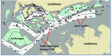
Figure 1 shows the e-navigation chart (ENC) of a strait. The ENC is composed of several features such as anchor-ages where vessels anchor and wait for services, berths, pilot boarding grounds, and the traffic separation scheme orTSS. The TSS (figure 1) is the set of mandatory unidirectional routes designed to reduce collision risk among vessels tran-sitioning through or entering the Strait. The TSS is
respon-Copyright c2019, Association for the Advancement of Artificial Intelligence (www.aaai.org). All rights reserved.
Landmass
Traffic Separation Scheme (TSS)
Zone markers
Anchorages
Landmass
Figure 1: Electronic navigation chart (ENC) of strait near a large asian city with color-coded features (best viewed elec-tronically)
sible for carrying the bulk of the maritime traffic. Therefore, we focus on traffic coordination in the TSS.
Based on geographical features, the TSS can be further di-vided into smallerzones(as shown in figure 1). Our goal is to compute the recommended time taken to cross each zone based on the current traffic in other zones such that (a) traffic intensity is within some pre-defined limit (which increases safety of navigation), and (b) maximize traffic throughput while maintaining the safety of navigation. E.g., if the path leading to berths is crowded (or the count of vessels is high), we may slow down vessels entering TSS to regulate the fic. We develop both the maritime traffic simulator and traf-fic control approaches.
by the ship condition, and weather conditions such as wind, rain and tides. Therefore, even if we provide a recommenda-tion to a vessel to cross a particular zone inT minutes, the actual time taken to cross is stochastic. It is not clear apriori how should we parameterize such uncertainty in the vessel movement. Hence, a micro-level simulation of the maritime traffic that simulates the precise position of each vessel is very challenging. In our work, we accommodate such unique maritime domain constraints in our traffic simulator and traf-fic coordination techniques.
Related work in maritime traffic management:For mar-itime traffic optimization, most current works either involve high fidelity commercial simulation tools to model micro-level navigation characteristics of vessels (Marin 2018), and expert systems and rule-based approaches to model the macro-level behavior of the traffic (Hasegawa et al. 2001; Hasegawa 1993; Ince and Topuz 2004). However, enhancing safety of navigation in a geographically constrained heavy traffic area, requires statistical modeling and learning from large amounts of historical data. Rule-based expert systems are not sufficient to resolve every possible close quarter sit-uation in the heavily trafficked Strait.
Related work in multiagent planning and learning:Our work can be cast as a decentralized partially observable MDP (Dec-POMDP) (Bernstein et al. 2002) which is a rich framework for sequential multiagent decision making. How-ever, solving even 2-agent Dec-POMDP is computationally challenging, being NEXP-Hard (Bernstein et al. 2002). To address scalability, previous works have explored several restricted variations of Dec-POMDPs (Becker et al. 2004; Spaan and Melo 2008; Witwicki and Durfee 2010). Re-cent works have focused on models where agent interactions are primarily dependent on agents’ “collective influence” on each other rather than their identities (Varakantham, Adulyasak, and Jaillet 2014; Sonu, Chen, and Doshi 2015; Robbel, Oliehoek, and Kochenderfer 2016; Nguyen, Ku-mar, and Lau 2017a; 2017b). In our work, we also explore this direction as vessels in maritime traffic can be consid-ered homogenous affecting each other only via their collec-tive presence (such as congestion). Colleccollec-tive decentralized POMDPs (CDec-POMDPs) have been proposed to model
such collective multiagent planning models (Nguyen, Ku-mar, and Lau 2017a). Existing works in CDec-POMDPs
assume that all agents act in synchronous manner with fixed duration actions (Nguyen, Kumar, and Lau 2017a; 2018). We extend theCDec-POMDP model to handle
asyn-chronous agent behavior with variable duration actions which helps to model real word settings (e.g., navigation to another zone has stochastic duration). There are multia-gent planning models with variable durations actions (Am-ato, Konidaris, and Kaelbling 2014). However they are lim-ited in scalability to a few agents as opposed to thousands of vessels or agents in the maritime domain. A determinis-tic scheduling approach exists for maritime traffic manag-ment (Agussurja, Kumar, and Lau 2018). However this ap-proach addresses a deterministic setting where each vessel follows the computed schedule exactly without any devi-ation. In our model, we address a more realistic model of vessel navigation based on stochastic duration actions.
In our work, we contribute the design and develop-ment of a maritime traffic simulator, and traffic control ap-proaches. Our simulator addresses several maritime domain constraints as highlighted earlier, and also allows for vari-able duration actions. We have access to 4 month histor-ical AIS (Automatic Identification System) data contain-ing timestamped position, speed over ground, direction, and navigation status (e.g., at anchor, not under command) of each vessel roughly every 10 seconds. The total dataset con-tains more than 9 million unique records. We process this dataset and use it to learn and validate several parameters of our simulation model. We also develop maritime traffic control approaches using a policy gradient approach that ex-ploits the collective nature of interactions among vessels. We test on synthetic domains and using our historical data based simulator to show that our approaches provide significant improvement over baseline approaches.
2
Model Definition
We next describe our model. The navigable sea space where traffic needs to be regulated (denoted asport waters) is di-vided into multiple zonesz ∈Z. We consider set of zones
˜
Z = Z ∪ {zd} including navigable zonesz ∈ Z, and a
dummy zonezd. The dummy zone indicates that the vessel is
outside the port waters. There are a total ofMvessel agents. An agentmcan be present in one of these zones. Zones can be arranged in the form of a directed acyclic graph in which each zone is a node, and edges correspond to traffic flow among zones. Such graph structure is typically determined by a VTS authority to separate outbound, inbound and tran-siting traffic. E.g., in figure 1, east-to-west and west-to-east are separated in the TSS.
Traffic enters the port waters via a set of specified source zonesZsrc⊂Z(e.g., extreme east or extreme west zones in
figure 1). Agents terminate their journey at a set of termi-nal zonesZter⊂Z, which for example may represent berths,
anchorages or transiting out of port water boundary. Vessels arrive in port waters over time; a vessel outside the port wa-ter boundary is assumed to be in a dummy zonezd. We have
discrete time, finite plan horizonH.
Traffic control: At each time stept, to regulate the conges-tion, atraffic control agentadvises a speedvzz0
t for vessels
moving from zonezto zonez0. We consider the speed
rec-ommendation as the output of a policy function parameter-ized using θ,πzz0
θ (•), taking input as joint-state of vessels
currently in port water. The objective of the traffic control agent is to optimize the parameters θ of the policy tion to optimize a congestion and delay based utility func-tion (defined later).
Vessel Model: We model the behavior of each vessel as fol-lows. Letsm
t denote the state of vesselmat timet. Consider
a vesselmcurrently inside the port waters. As the naviga-tion acnaviga-tion has a variable duranaviga-tion, this vessel can be catego-rized asnewly arrivedat some zonezat timetorin-transit
throughzatt.
• In-transit: sm
t =hztm, zt0m, τmiwhereztm∈Z denotes
vessel’s current zone at timet,z0m
agent is heading to, andτmis the future time at which the
vessel reaches the next zonez0m t .
• Newly arrived:When the vessel is newly arrived at zone zm
t , its next zonez0 and next arrival time τ are not yet
determined, and its statesm
t is denoted ashzmt ,∅,∅i.
Direction decision: When a vessel isnewly arrivedat zone zat timet(sm
t =hz, φ, φi), it will decide the next zonez0
from the distributionα(z0|z), and its actionam
t =z0. In
sev-eral ports, often the number of destinations vessels are head-ing to are small (e.g., berths, anchorages, transithead-ing through). Often, there are only very few navigation routes to reach such destinations which are decided by factors such as the TSS, and hydrological features such as deep water routes for deep draft vessels. Therefore, unlike routing in road net-works, we model theaveragenavigation behavior of vessels. We learn the distributionα(z0|z)from historical data, and
consider it as a fixed input model parameter. When a vessel isin-transit, its action isnulloram
t =∅.
Arrival distribution:To model the arrival timeτof vessels into the source zoneszsrc∈Zsrcfrom outside the port waters,
we assume a distribution{P(hzd, zsrc, τi)}zsrc∈Zsrc,τ∈[1:H].
We estimate this distribution from historical data. The start-ing state hzd, zsrc, τiimplies that the vessel moves to the
source zonezsrcat timeτ. Before timeτ, the vessel is
out-side the port waters. We assume that this arrival probability cannot be controlled as it is often determined by exogenous factors such as the schedule of the shipping line.
We have made the design choice topre-samplethe arrival timeτ at the vessel’s next destination because vessels can take variable amount of time to cross a zone. Therefore, at any instant in time, we have to record how many vessels are currently transiting through a zone to accurately compute the reward, and determine future adjustments of vessel speeds depending on the current traffic.
State transition functionφ:We define the state transition function for a vessel as follows:
• If vesselmis currently outside the port waters orsm
t =
hzd, zsrc, τi, thenφ(smt+1=hzsrc, φ, φi|smt ) = 1ift+1 =τ,
otherwise zero. If(t+ 1)< τ, then vessels remains in the same statehzd, zsrc, τiwith probability 1.
• If vesselmis inside the port waters, and has newly ar-rived at a zone z at time t or sm
t =hz,∅,∅i, it would
choose next zone z0 from the distribution α(z0|z), and
the arrival timeτ atz0 is sampled from the distribution
pnav(τ|z, z0;βzz0
t )whereβzz 0
t is the speed control
param-eter for moving fromztoz0at timet. We will show later howβis determined, and the parametric form of distribu-tionpnav. Therefore, ifsm
t =hz,∅,∅i; smt+1=hz, z0, τi,
thenφ(sm t+1|s
m
t ;βt) =α(z0|z)·p
nav(τ|z, z0;βzz0 t ).
• If agentmis in-transit from zoneztoz0at timetorsm
t =
hz, z0, τi, then two cases can happen. At timet+ 1, the
agent finally crosses zonezand reaches the starting point of zonez0. This setting occurs whenτ=t+ 1(recall that
τ denotes the arrival time at zone z0). Other case is the
agent is still in-transit through zonezat timet+ 1. This occurs whenτ > t+ 1. The caseτ < t+ 1is inconsistent
as it implies the agent reaches its destination in the past.
φ(smt+1|s
m t ;βt) =
I(smt+1=hz0,∅,∅i) iffτ=t+ 1
I(smt+1=hz, z0, τi) iffτ > t+ 1
(1)
whereIis the indicator function giving one or zero based
on its input logical condition being true or false.
For ease of exposition, we have not shown the transition function for terminal zoneszter∈Zter. When the agent first
enters anyzter, say at timet, its state ishzter,∅,∅i. It is an
absorbing state with zero reward, no outgoing transitions. Count statistics: To summarize the joint activities of
ves-selsst,at=hstm, amt ∀m= 1 :Miat each time stept, we
consider the aggregate statistics as follows:
• ntxn
t (z, z0, τ)=
PM
m=1I(s
m
t =hz, z0, τi)∀z, z0∈Z, τ > t.
It counts the vessels that are currently in-transit in zonez and will reach zonez0at timeτ.
• narr
t (z)=
PM
m=1I(s
m
t =hz,∅,∅i)∀z∈Z. It counts
ves-sels that newly arrived in zonezat timet.
• nnxt
t (z, z0)=
PM
m=1I(s
m
t =hz,∅,∅i;amt = z0)∀z, z0∈
Z. It counts vessels that newly arrived in zone z at the current timetand decided to go to zonez0. We also have
the consistency relation:narr
t (z) =
P
z0nnxtt (z, z0)
• n˜t(z, z0, τ)=P M m=1I(s
m
t = hz, φ, φi, amt = z0, smt+1 =
hz, z0, τi) ∀z, z0∈Z, τ > t. It counts vessels that newly
arrived in zonez at the timet, decided to go toz0, and
reachingz0at timeτ.
• From the above counts, we can compute the total number of agents present in each zonezat timetwhich include both newly arrived and in-transit agents as:
ntott (z) = n
arr
t (z) +
X
z0∈Z,τ=t+1:H
ntxnt (z, z0, τ) (2)
We arrange the above counts in the form of tables. E.g.,
ntot
t = (ntott (z) ∀z ∈ Z). Analogously, we define
the count tables ntxn
t ,n
arr
t ,n
nxt
t ,n˜t. We denote nt =
(ntxn
t ,narrt ,nnxtt ,˜nt)to be the count table vector at each time
tandn1:Hto be joint tables from timet= 1toH.
Reward: The reward at time t depends on the aggregate count of agents in different zones. We treat each zonez as a limited capacity resource. The reward function balances the consumption of this resource and any potential delay caused to vessels. The capacitycap(z)of this resource, for example, indicates how many maximum number of vessels can besafelypresent in the particular zone. For simplicity, we assume that each vessel consumes one unit of resource. When the capacity of the resource is violated, a penalty is imposed on each involved vessel. To also ensure that vessel reach their destination as soon as possible, there is a delay penalty per vessel for each time step. Hence, the rewardrm t
of a vesselmat zonezis computed as:
rm
t =−C(z,n
tot
t ) =−
wr·max ntott (z)−cap(z), 0
+wd
(3) where wr and wd are positive weights; wr penalizes
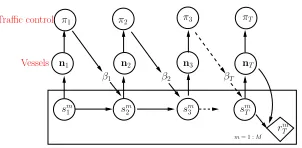
βT β2 β1
n2 n3 nT
sm
1 sm2
rm T π1
m= 1 :M Vessels
Traffic control
sm T sm
3
n1
π3
π2 πT
Figure 2: Dynamics of Maritime Traffic Control
The overall rewardrcan be computed by aggregating local rewards of vessels in different zones as follows:
r(nt) =−
X
z∈Z
ntott (z)·C(z,n
tot
t ) (4)
Traffic control objective:Lets1:T,a1:T={sm1:T, a m
1:T ∀m}
denote the joint T-step trajectory of agents resulting in counts n1:T. The objective function for the traffic control
agent is to maximize:
V(πθ) = H
X
T=1
Es1:T,a1:T[r(nT)|aT,sT;πθ] (5)
Figure 2 shows the dynamic Bayesian net of our maritime traffic model with the traffic control agent (TCA) provid-ing speed guidance usprovid-ing the policy π at each time step. The control policy πtakes as input the joint counts nt at
each time step, and provides traffic control guidanceβt =
{βzz0
t ∀z, z0}, which regulates vessel navigation using the
distributionpnav(·|z, z0;βzz0 t )∀z, z0.
Modeling vessel navigation behavior (pnav, βzz0):A
cru-cial aspect to address is modeling the navigation behavior of vessels. If a vessel navigating (z → z0) is given an
recom-mendation by the traffic control agent (TCA) to perform this entire navigation inµtime periods, then would this vessel finish this action in exactlyµtime periods or requireµ±δ whereδis a random variable to take into account stochastic-ity of real world navigation? Furthermore, we must impose hard travel time limitstminandtmaxto model maximum and
minimum speeds. As there are currently no controlled exper-iments with real vessels, there is no historical data to learn from. To address this issue and avoid making any unneces-sary assumptions, we use theprinciple of maximum entropy
(Maxent) (Jaynes 1957). The maxent principle advocates for the distribution that respects given constraints on parame-ters, but avoids making any other unnecessary assumption to avoid overfitting. Such maxent distributions have been used in computational sustainability to model dynamics of endangered species given that their observations are sparse and incomplete (Phillips, Anderson, and Schapire 2006).
We interpret the parameterβzz0 as specifying the travel
time∆(βzz0)recommended by the TCA to move fromzto
z0. Weassumethat given this recommendation, theaverage
travel time of vessels would be∆(βzz0). However, the actual
travel time of individual vessels can be different. Some may cross in less time than∆and some may take more. Notice that our assumption is realistic. If on-an-average, vessels do not follow traffic guidance, then it would be virtually impos-sible to control the traffic. This is where the role of a VTS
authority comes in—as a traffic regulatory authority, it may be possible to incentivise vessels to follow the navigation recommendations.
The travel time distributionpnav(τ|z, z0;βzz0)is the
max-imum entropy distribution with mean∆(βzz0). It has been
shown that the maxent discrete probability distribution with bounded positive support and a specified mean is the bi-nomial distribution(Harremoes 2001). We incorporate hard limitstminandtmaxon the output ofpnavas follow.
Let current time bet. For(z → z0), the arrival time at z0 isτ=t+ (tzz0
min+ ˜∆). We sample∆˜ from the binomial
distribution with(tzz0
max−tzz
0
min)trials and success probability
of each trial beingβzz0
t (or the output of the TCA policyπ).
That is,∆˜ ∼B(tzz0
max−tzz
0
min, βzz
0
t ). The average travel time
is ∆(βzz0
) = tzz0
min+ (t
zz0
max−t
zz0
min)β
zz0
t , a standard result
for binomial distribution. In experiments, we provide empir-ical support by using historempir-ical data, and showing that our simulator built on the binomial distribution gives very close vessel traffic distribution to the real historical data for mul-tiple days over peak traffic hours.
3
Generative Model for Counts
While, we can optimize objective (5) by sampling joint state-action trajectories of all the agents. This approach is not scal-able as typically more than a thousand vessel cross the Strait each day. Integrating sampling of individual agent trajecto-ries within a reinforcement learning based simulator is com-putationally intractable. Therefore, we reparameterize value function using countsn1:H, and show that counts are
suffi-cient statistic for planning in our traffic control model. Sam-pling countsn1:H is highly scalable as even if the number
of vesselsM increases, the dimensions of the count table re-mains fixed. Only the count of vessels in different buckets of count tables changes. As discussed in the previous section, letnt= (ntxnt ,n
arr
t ,n
nxt
t ,˜nt)denote the count table vector.
We first show thatn1:H are sufficient statistic for the joint
distribution over state-actions trajectories of agents. Theorem 1. Count vectorn1:His the sufficient statistics for the joint distributionP(s1:H,a1:H;π)
Proof. Notice that a vessel takes the action to move to an-other zonez0and samples its travel duration frompnavonly
when it is in a newly arrived state hz, φ, φi(for some z). We can summarize this transition using the indicator func-tion I(smt =hz, φ, φi, amt =z0, smt+1 =hz, z0, τi). Rest of
the state transitions are deterministic. E.g., when a vessel is in-transit, it moves to its destinationz0at timeτwith
proba-bility1. We use this fact to aggregate vessels’ states into the counts as follow:
P(s1:H,a1:H) =
M Y
m=1
H Y
t=1
Y
z,z0,τ
α(z0|z)
×pnav(τ|z, z0,βt=πt(nt))I(s m
t=hz,φ,φi,amt=z0,smt+1=hz,z0,τi
=Y
t
Y
z,z0,τ
α(z0|z)pnav(τ|z, z0,βt=πt(nt))
˜nt(z,z0,τ) (6)
where we used the fact that n˜t(z, z0, τ)=P M m=1I(s
m
t =
hz, φ, φi, am
see that countsnare the sufficient statistic as (6) only de-pends on the counts generated by any(s1:H,a1:H).
Generating counts: We next show the generative model for nt+1 = (narrt+1,nnxtt+1,˜nt+1,ntxnt+1) given nt. Total
ves-sels newly arriving in zone z0 at time t+ 1, narr
t+1(z0), is
given by the sum of vessels that were in-transit toz0 at time
t (or ntxn
t (z, z0, τ =t+ 1)), and newly arrived vessels in
a zone z with next destination z0 reaching z0 at t+ 1(or ˜
nt(z, z0, τ=t+1)).
narr
t+1(z
0) =X
z [ntxn
t (z, z
0, τ=t+1)+˜n
t(z, z0, τ=t+1)]∀z0
(7)
nnxt
t+1: Given narrt+1, we can generate next zone counts
nnxt
t+1(z,·)from a multinomial distribution with parameters
pz0=α(z0|z)∀z0as below:
nnxt
t+1(z,·)| narrt+1(z)∼Mul(narrt+1(z), pz0∀z0) (8)
˜
nt+1: Next we sample the arrival time counts in destination
zonesz0. That is, for all newly arrived vessels atzmoving to
z0, we sample the countsn˜
t+1(z, z0,·). Given that vessels’
navigation time follows a binomial distribution (orpnav is
binomial), we sample from a multinomial distribution with parameterspτ=pnav(τ|z, z0;βzz
0 t+1)∀τ
˜
nt+1(z, z0,·)| nnxtt+1(z, z0)∼Mul(n nxt
t+1(z, z0), pτ∀τ) (9)
where,τ=t+ 1 +tzz0
min+ ˜∆,∆˜ ∈[0, t
zz0
max−t
zz0
min]
Based on above counts, we compute all vessels that are in-transit to other zonesz0at timet+ 1. It includes all vessels in-transit at timetreaching their destination at timeτ > t+1, and newly arrived vessels˜nt(z, z0, τ)in-transit toz0.
ntxn
t+1(z, z
0, τ) = ntxn
t (z, z
0, τ)+˜n
t(z, z0, τ)∀z, z0,∀τ > t+1
(10)
Using above process, we can sample all countsn1:H
with-out sampling individual vessel trajectories. Sampling from such multinomial distributions remains efficient even if the vessel population increases. This makes such count-based sampling significantly more scalable than sampling individ-ual agent trajectories. We show in appendix the exact distri-bution over counts orP(n1:H). We refer to constraints
(7)-(10) which every count table must satisfy asΩ1:T.
4
Vessel-Based Value Function
As countsn1:Hare sufficient statistic for the distribution of
joint state-action trajectories, and given the generative distri-butionP(n1:H)over counts, we have (proof in appendix):
Theorem 2. The traffic control objective in(5)can be com-puted by expectation over counts
V(πθ) =
H X
t=1
Es1:t,a1:t[r(nt)|at,st;πθ] = H X
t=1
En1:t∈Ω1:t
r(nt)|πθ
We can directly optimize the above objective by com-puting gradient ∇θV(πθ) using stochastic gradient ascent
and moving parameters θ in the direction of the gradient.
This strategy is similar to the well known REINFORCE policy gradient approach in RL (Williams 1992). How-ever, we show empirically that this approach does not work well. The reason is the problem of multiagent credit as-signment (Chang, Ho, and Kaelbling 2004; Bagnell and Ng 2006). That is, from the global reward signalrtit is not clear
which agent should get the credit or penalty for the overall traffic state. Instead, we consider a vehicle-based value func-tion framework (Wiering 2000; Bakker et al. 2010) to train traffic control policy. Letπ=hπzz0
θ ∀z, z0i. Eachπzz 0 θ outputs
the speed control parameterβzz0
t at each timet. We assume
the crossing zz0 is like a traffic light, and compute the
to-tal accumulated reward (from timettillH), sayVzz0 t (πzz
0 θ ),
for those vessels that newly arrive at zonez at timetand decide to move toz0. Originally, in (Wiering 2000),
vehicle-based method requires the joint state-actions of all vehicles at every time step.
Vzz0 t (π
zz0 θ ) =E
M
X
m=1
I[smt =hz,∅,∅i, a m t =z
0]
H
X
t0=t
rm t0
πθ
(11)
Under this vessel-based traffic control framework, we op-timize each Vzz0
t (π zz0
θ ) in an iterative fashion, similar to
car-based value functions in (Wiering 2000). This is an ap-proximate solution technique, but is known to produce good road traffic control policies (Bakker et al. 2010), and empir-ically, we observed it works significantly better than the RE-INFORCE method asVzz0
t performs effective credit
assign-ment computing precisely the effectiveness of policy πzz0 θ
by filtering out the contributions from other zone pairs. In our model, we work at the abstraction of counts, and thus extracting joint state-action trajectories for each vessel is expensive, and not scalable for large agent population. We therefore develop a collective vessel-based value function mechanism to compute this value using only the counts.
Theorem 3. The vehicle-based value function can be com-puted by collective expectation over the counts as follows:
Vtzz0(π zz0
θ ) =En1:H X
τ >t ˜
nt(z, z0, τ)Vtn(z, z0, τ)
πθ
(12)
in whichVn
t (z, z0, τ)is the average accumulated reward of newly arrived vessels at z at timet going to z0 computed based on the realized countsn1:Has follows:
Rtn(z, z 0
, τ) =
τ−1
X
τ”=t
−C(z,ntotτ”),∀τ∈[t+tzz 0
min, t+tzz 0 max] (13)
Vn
t (z, z
0, τ) =R
t(z, z0, τ) +γ·Vτn(z
0) (14)
Vtn(z, z 0
) =
Pt+tzz 0
max
τ=t+tzz0
min
Vtn(z, z0, τ)·˜nt(z, z0, τ)
Pt+tzz 0
max
τ=t+tzz0
min
˜
nt(z, z0, τ)
(15)
Vtn(z) = P
z0nnxtt (z, z0)·Vtn(z, z0)
P
z0nnxtt (z, z0)
, (16)
whereRn
t(z, z0, τ)is the reward accumulated by a vessel when it is still in zonezbetween timetandτ;Vn
the average accumulated reward of a vessel which started crossingztoz0from timet.Vn
τ(z0)is the average accumu-lative reward of a vessel newly arrived atz0at timeτ.
Proof is provided in the appendix. Such vessel-based value function can be computed using a dynamic program-ming approach. We next compute the gradient of this vessel-based value function below (derivation in appendix):
Theorem 4. The vehicle-based policy gradient forπzz0 is
∇θVzz 0
1 (π
zz0
θ ) =En1:H
h X
t=1:H t+tzz0
max
X
τ=t+tzz0
min ˜
nt(z, z0, τ)×
(τ−t−tzz0
min)· ∇θlog(πzz
0
θ (nt)) + (tzzmax0 −(τ−t))· ∇θlog(1−πzz
0
θ (nt))
Vtn(z, z0, τ)
i
(17)
After computing above policy gradients, we can aggregate all∇θVzz
0
1 and update the policy parameterθas follows:
θnew←θold+γX
z,z0
∇θVzz 0
1 (π
zz0
θ ) (18)
whereγis the learning rate. We call this approach as vessel-based policy gradient(orVessel-PG). Our results are devel-oped for the general setting where traffic control policyπzz0
takes as input all the count informationnt. However,
empir-ically we observed that providing only total vessel counts in zonezandz0,(ntot
t (z),ntott (z0)), as input provided higher
quality solutions. Another benefit of such a policy is that it is easily implementable in a decentralized setting. Vessels have radars which can provide information about count of other vessels in their current zonez, and their next destina-tion zonez0. Thus, vessels can query the policyπbased on
their local observations to get their speed control input.
5
Experimental Results
We perform experiments on both synthetic and real-world instances. Synthetic instances are for comparison against different methods by varying problem sizes, while real-world instances are used to evaluate effectiveness of our ap-proach on mitigating hotspots within the strait. A detailed description about all experimental setups (policy structure, and other settings) are provided in the appendix.
Baselines :We compare our approachVessel-PGwith three baselines—deep deterministic policy gradient (DDPG) (Lil-licrap et al. 2015), policy gradient (PG) and MaxSpeed. As DDPG is for MDPs, we first extend the DDPG algorithm to our setting (details on this extension are in appendix). PG is standard policy gradient (REINFORCE) approach where we train with total empirical returns, and MaxSpeed policy is to always travel a zone with maximum uniform speed cor-responding totzz0
mintravel time for the zone pair.
Synthetic Data :For each synthetic instance, we generate a semi-random connected directed graph with edges repre-senting zones, similar to (Agussurja, Kumar, and Lau 2018). With each edge is associated a minimum and a maximum time required to traverse the edge. Vessels arrive at traffic
source edges with an arrival rate. The resources are the edge capacities (or the maximum number of vessels on an edge at any instant). Other problem settings are in the appendix.
Figures (3a-3c) show results with varying resource penaltywr, 100 vessels and maximum capacity of each edge
as 5. In all three, a lower value is better, y-axis is in log-scale. Figure 3b shows resource violations, figure 3c shows the total average delay over the MaxSpeed policy (i.e., if all vessels travel at the maximum speedtmin, delay is zero); and
figure 3a shows the overall objective we optimize in (3) (we convert rewards to costs, therefore lower cost is better). The resource violation value in figure 3b is sum of violations at each time step for the whole horizon. In figure 3c, MaxSpeed baseline is not shown as delay is 0. We also see similar be-havior of close to 0 delay withVessel-PGonwr= 0, which
is also intuitive as wr = 0 ignores the resource violation
component in the objective; DDPGalso achieves a close to optimal policy, but has slightly higher resource violations
thanVessel-PGfor this case. Delay increases with
increas-ing value ofwrbecause optimization preference shifts more
towards violation. In all three settings of wr, Vessel-PG
achieves significantly better solution quality (i.e. lower de-lay). Similar behavior is also observed in figure 3b as vio-lation of MaxSpeed, Vessel-PGandDDPGare similar at wr = 0 and violations decreases with increasing resource
penalty value. Crucially,Vessel-PGdecreases resource vio-lations faster than DDPG, and PG highlighting the effective-ness of our approach. Figure 3a results are the actual objec-tive value that we optimize for, which subsumes both viola-tion and delay components. We observeVessel-PGachieves significantly better solution quality than rest of the baselines. Figure 3d results are for 100 vessels, resource penalty wr= 5andwd= 1. We set a threshold capacity as 50 for
any edge (or 50% of total number of vessels), and vary ac-tual resource capacity as a percentage of this threshold ca-pacity. Y-axis shows the objective value (lower is better). In all the four settings of capacity% we seeVessel-PG achiev-ing better solution quality than the rest, quality gap among all approaches reduces as the capacity% increases. This is because problem instance becomes easier as resource viola-tions go to zero with increased capacity%. Figures 3e shows results with varying number of vessels, resource capacity as 5 for each edge and wr= 5, wd = 1. In this case also,
ca-0 1 5
ResourcePenalty(w_r)
1000 10000 100000 O b je ct iv e Vessel-PG DDPG PG Max.Speed
(a)Objective (log scale)
0 1 5
ResourcePenaly(w_r) 10 100 1000 10000 V io la ti on
Vessel-PG DDPG PG Max.Speed
(b)Resource violations (log-scale)
0 1 5
ResourcePenalty(w_r) 1 10 100 1000 Av g. D e la y (i n m in
.) Vessel-PG DDPG PG
(c)Average delay (log-scale)
10 20 60 80
ResourceCapacity(in%) 1000 10000 100000 1000000 O bje ct iv e Vessel-PG DDPG PG Max.Speed
(d)Varying resource capacity
50 100 300 400
Total Vessels 100 1000 10000 100000 1000000 10000000 O b je ct iv e Vessel-PG DDPG PG Max.Speed
(e)Varying number of vessels
2 4 6 8 10 12 14 16 18 20 22 24
HouroftheDay 0 20 40 60 80 100 120 140 160 A v g. T r af � ic Int ensity
Avg.Traf�icIntensityover4months
1 2 3 4 5 6 7 8 9 10
Day 0 2 4 6 8 10 Max. Violation Unsch. Sch. 4thHour,60%Cap
(f)Traffic intensity; 4th hour violations
1 2 3 4 5 6 7 8 9 10 Day 0 2 4 6 8 10 12 14 Max. Violation Unsch. Sch. 5thHour,60%Cap
1 2 3 4 5 6 7 8 9 10 Day 0 2 4 6 8 10 12 Max. Violation Unsch. Sch. 6thHour,60%Cap
(g)5th, 6th hour violations
1 2 3 4 5 6 7 8 9 10 Day 0 1 2 3 4 5 6 7 Max. Violation Unsch. Sch.
7thHour,60%Cap
1 2 3 4 5 6 7 8 9 10 Day 0 1 2 3 4 5 Max. Violation Unsch. Sch.
8thHour,60%Cap
(h)7th, 8th hour violations
1 2 3 4 5 6 7 8 9 10
Days 0 50 100 150 200 250 A v g. T r a v el Time(in min.)
Unsch. Sch. (60% Cap)
(i)Avg. travel time with varying capacity
Figure 3: (a-e) show results for synthetic instances (lower value is better). (f-i) show quality comparisons on historical data
pacitiescap(z)over 4 months data,tzz0
min andt
zz0
max are also
estimated, resource penaltywr = 50(after some
trial-and-error this value worked best), delay penaltywd = 1. We
divide an hour period into 60 time steps (1 minute inter-vals); time step 0 is 12AM. Vessel’s arrival rate are com-puted from data for each day. We experiment with 60% of historicalcap(z)to test how to reduce traffic intensity, and its impact on travel time.
Simulator Accuracy: We wanted to show that our simu-lator provides very similar peak traffic window and trend as the real data. We have computed root mean square error (RMSE) as a more concrete accuracy measure. For 12 (out of a total of 27 zones) high traffic intensity zones for peak hour window. On average over 4 months, the RMSE value is around 1.8, which intuitively means that on average there is a difference of 1.8 vessels between predicted count and observed count at each time step. On an average, around 50 vessels cross any of these 12 zones during the peak hour; thus the RMSE of 1.8 is relatively low. Figures are provided in appendix section 3
Peak traffic intensity reduction: Figures (3f-3i) show real data experiments. Figure 3f(top) shows traffic intensity for the whole planning area averaged over 4 months period, y-axis is number of unique vessels present in the planning area for each hour period, x-axis shows hours of the day. We can see that peak hours are at 4th, 5th and 6th. Therefore, for each day we apply our method (Vessel-PG) to control for this 3 hour window. Figures 3f(bottom)–3h(bottom) show results for 4th-8th hours, y-axis shows the maximum vio-lation for that hour, x-axis shows the day number, legend Schis our method andUnschis the observed values from data. As noted, we control only 4th-6th hour window; for 7th and 8th hour we useβzz0
datato simulate future traffic for
our method. We have added these two additional hours to show if there is any shift of peak hour, which would be unde-sirable. Results show significant reduction in violations for all 10 days on all hours except 8th hour (figure 3h(bottom)).
Even though traffic intensity for 8th hour has increased by our method, the increase is only marginal, significantly less than the reduction in peak traffic intensity reduction for 4th-7th hour. Therefore, our traffic control strategy is highly ef-fective, and does not shift peak traffic intensity.
Next we assess how traffic throughput is impacted by our traffic control method. Figure 3i shows average travel time a vessel would take if it entered the planning zone between 4th - 8th hour window (starting of our traffic control) trav-eling on the longest west-east route in TSS. We observe that travel time reduces with our method for all days sig-nificantly. Notice that our results imply that vessels should move at a higher speed (within the defined thresholds im-plied bytmin,tmax) within TSS, which would lead to a
re-duction in resource violations (implying safer traffic), and also would reduce travel time.
6
Conclusion
We addressed the problem of maritime traffic management in busy waterways of strait near a large asian city. Based on historical data, we have developed and validated a mar-itime traffic simulator. Using this simulator, which models aggregate behavior of vessels, we developed a policy gradi-ent approach that provides speed guidance to vessels. Em-pirically, our approach works much better than competing approaches, and shows the potential of coordinating traffic for better navigation safety with high traffic throughput.
7
Acknowledgments
References
Agussurja, L.; Kumar, A.; and Lau, H. C. 2018. Resource-constrained scheduling for maritime traffic management. InAAAI Conference on Artificial Intelligence.
Amato, C.; Konidaris, G.; and Kaelbling, L. P. 2014. Planning with macro-actions in decentralized POMDPs. InInternational confer-ence on Autonomous Agents and Multi-Agent Systems, 1273–1280. Bagnell, D., and Ng, A. Y. 2006. On local rewards and scaling distributed reinforcement learning. InAdvances in Neural Infor-mation Processing Systems, 91–98.
Bakker, B.; Whiteson, S.; Kester, L.; and Groen, F. C. A. 2010. Traffic Light Control by Multiagent Reinforcement Learning Sys-tems. Springer Berlin Heidelberg. 475–510.
Becker, R.; Zilberstein, S.; Lesser, V.; and Goldman, C. V. 2004. Solving transition independent decentralized Markov decision pro-cesses.Journal of Artificial Intelligence Research22:423–455. Bernstein, D. S.; Givan, R.; Immerman, N.; and Zilberstein, S. 2002. The complexity of decentralized control of Markov decision processes.Mathematics of Operations Research27:819–840. Chang, Y.; Ho, T.; and Kaelbling, L. P. 2004. All learning is lo-cal: Multi-agent learning in global reward games. InAdvances in Neural Information Processing Systems, 807–814.
Hand, M. 2017. Malacca and S’pore Straits traffic hits new high in 2016, VLCCs fastest growing segment. http://www.seatrade- maritime.com/news/asia/malacca-and-s-pore-strait-traffic-hits-new-high-in-2016-vlccs-fastest-growing-segment.html.
Harremoes, P. 2001. Binomial and poisson distributions as max-imum entropy distributions. IEEE Transactions on Information Theory47(5):2039–2041.
Hasegawa, K.; Tashiro, G.; Kiritani, S.; and Tachikawa, K. 2001. Intelligent marine traffic simulator for congested waterways. In IEEE International Conference on Methods and Models in Au-tomation and Robotics.
Hasegawa, K. 1993. Knowledge-based automatic navigation sys-tem for harbour manoeuvring. InShip Control Systems Symposium, 67–90.
Ince, A. N., and Topuz, E. 2004. Modelling and simulation for safe and efficient navigation in narrow waterways. Journal of Naviga-tion57(1):53–71.
Jaynes, E. T. 1957. Information theory and statistical mechanics. Phys. Rev.106(4):620–630.
Liang, A., and Maye-E, W. 2017. Busy waters around Singapore carry a host of hazards. https://www.navytimes.com/news/your- navy/2017/08/22/busy-waters-around-singapore-carry-a-host-of-hazards/.
Lillicrap, T. P.; Hunt, J. J.; Pritzel, A.; Heess, N.; Erez, T.; Tassa, Y.; Silver, D.; and Wierstra, D. 2015. Continuous control with deep reinforcement learning.arXiv preprint arXiv:1509.02971. Lim, V. 2017. 300 tonnes of oil spilled after Singapore-registered ship collides with vessel off Johor. http://www.channelnewsasia.com/news/singapore/300-tonnes-of-oil-spilled-after-singapore-registered-ship-collid-7537142. Marin. 2018. MARIN: Vessel Traffic Service (VTS) Simulators. http://www.marin.nl/web/Facilities-Tools/Simulators/ Simulator-Sales/Vessel-Traffic-Service-VTS-Simulators.htm. Nguyen, D. T.; Kumar, A.; and Lau, H. C. 2017a. Collective multi-agent sequential decision making under uncertainty. InAAAI Con-ference on Artificial Intelligence, 3036–3043.
Nguyen, D. T.; Kumar, A.; and Lau, H. C. 2017b. Policy gra-dient with value function approximation for collective multiagent
planning. InAdvances in Neural Information Processing Systems, 4322–4332.
Nguyen, D. T.; Kumar, A.; and Lau, H. C. 2018. Credit assignment for collective multiagent RL with global rewards. InAdvances in Neural Information Processing Systems.
Phillips, S. J.; Anderson, R. P.; and Schapire, R. E. 2006. Maxi-mum entropy modeling of species geographic distributions. Eco-logical Modelling190(3):231 – 259.
Robbel, P.; Oliehoek, F. A.; and Kochenderfer, M. J. 2016. Ex-ploiting anonymity in approximate linear programming: Scaling to large multiagent MDPs. InAAAI Conference on Artificial Intelli-gence, 2537–2543.
Segar, M. 2015. Challenges of Navigating In Congested and Restricted Water. http://www.mpa.gov.sg/web/wcm/ connect/www/968fafb8-7582-4091-9bcd-ec0a332f73a6/
segar challenges of navigating.pdf.
Sonu, E.; Chen, Y.; and Doshi, P. 2015. Individual planning in agent populations: Exploiting anonymity and frame-action hyper-graphs. InInternational Conference on Automated Planning and Scheduling, 202–210.
Spaan, M. T. J., and Melo, F. S. 2008. Interaction-driven Markov games for decentralized multiagent planning under uncertainty. In International COnference on Autonomous Agents and Multi Agent Systems, 525–532.
Tan, A. 2017. Big cleanup of Singapore’s north-eastern coast after oil spill. http://www.straitstimes.com/singapore/environment/big-cleanup-of-n-e-coast-after-oil-spill.
Varakantham, P.; Adulyasak, Y.; and Jaillet, P. 2014. Decentral-ized stochastic planning with anonymity in interactions. InAAAI Conference on Artificial Intelligence, 2505–2512.
Wiering, M. 2000. Multi-Agent reinforcement learning for traffic light control. InInternational Conference on Machine Learning, 1151–1158.
Williams, R. J. 1992. Simple statistical gradient-following algo-rithms for connectionist reinforcement learning.Machine Learning 8(3):229–256.