Stochastic Canonical Correlation Analysis

Stochastic Canonical Correlation Analysis

Chao Gao [email protected]

University of Chicago Chicago, IL 60637, USA

Dan Garber [email protected]

Technion – Israel Institute of Technology Haifa, 3200003, Israel

Nathan Srebro [email protected]

Toyota Technological Institute at Chicago Chicago, IL 60637, USA

Jialei Wang [email protected]

University of Chicago Chicago, IL 60637, USA

Weiran Wang [email protected]

Toyota Technological Institute at Chicago Chicago, IL 60637, USA

Editor:John Shawe-Taylor

Abstract

We study the sample complexity of canonical correlation analysis (CCA), i.e., the number of samples needed to estimate the population canonical correlation and directions up to arbitrarily small error. With mild assumptions on the data distribution, we show that

in order to achieve -suboptimality in a properly defined measure of alignment between

the estimated canonical directions and the population solution, we can solve the empir-ical objective exactly with N(,∆, γ) samples, where ∆ is the singular value gap of the

whitened cross-covariance matrix and 1/γ is an upper bound of the condition number of

auto-covariance matrices. Moreover, we can achieve the same learning accuracy by drawing the same level of samples and solving the empirical objective approximately with a stochas-tic optimization algorithm; this algorithm is based on the shift-and-invert power iterations and only needs to process the dataset forO log1

passes. Finally, we show that, given an estimate of the canonical correlation, the streaming version of the shift-and-invert power iterations achieves the same learning accuracy with the same level of sample complexity, by processing the data only once.

Keywords: Canonical correlation analysis, sample complexity, shift-and-invert precon-ditioning, streaming CCA

1. Introduction

Let x ∈ _Rdx _{and y ∈}

Rdy be two random vectors with a joint probability distribution P(x,y). The objective of CCA (Hotelling, 1936) in the population setting is to find u ∈

Rdx and v ∈ Rdy such that projections of the random variables onto these directions are

c

maximally correlated:1

max

u,v

E[(u>x)(v>y)]

p

E[(u>x)2]pE[(v>y)2]

. (1)

This objective can be written in the equivalent constrained form

max

u,v u

>_E

xyv s.t. u>Exxu=v>Eyyv= 1 (2)

where the cross- and auto-covariance matrices are defined as

Exy =E[xy>], Exx =E[xx>], Eyy =E[yy>]. (3)

The global optimum of (2), denoted by (u∗,v∗), can be computed in closed-form. Define

T:=E− 1 2 xx ExyE

−1 2

yy ∈Rdx×dy, (4)

and let (a1,b1) be the (unit-length) top left and right singular vector pair associated with T’s largest singular value ρ1 = σ1(T). Then the optimal objective value, i.e., the canonical correlation between x and y, isρ1 ≤1 (see Lemma 20), achieved by (u∗,v∗) = (E−

1 2 xxa1,E

−1 2 yy b1).

In practice, we do not have access to the population covariance matrices, but observe samples pairs (x1,y1), . . . ,(xN,yN) drawn from P(x,y). In this paper, we are concerned with both the number of samples N() needed to approximately solve (2), and the time complexity for obtaining the approximate solution. Note that the CCA objective is not a stochastic convex program due to the ratio form (1), and standard stochastic approximation methods do not apply (Arora et al., 2012). Globally convergent stochastic optimization of CCA has long been a challenge even for the empirical objective, and attracted continuous effort (Lu and Foster, 2014; Ma et al., 2015; Wang and Livescu, 2016), until the recent breakthrough by Ge et al. (2016); Wang et al. (2016). And our understanding of the stochastic objective, e.g., the existence of an efficient algorithm and the sample complexity, has been very limited.

Our contributions The contributions of our paper are summarized as follows.

• First, we provide the ERM sample complexity of CCA. We show that in order to achieve -suboptimality in the alignment between the estimated canonical directions and the population solution (relative to the population covariances, see Section 2), we can solve the empirical objective exactly withN(,∆, γ) samples where ∆ is the singular value gap of the whitened cross-covariance and 1/γ is a upper bound of the condition number of the auto-covariance, for several general classes of distributions widely used in statistics and machine learning.

• Second, to alleviate the high computational complexity of exactly solving the empirical objective, we show that we can achieve the same learning accuracy by drawing the same level of samples and solving the empirical objective approximately with the stochastic optimization algorithm of Wang et al. (2016). This algorithm is based on the shift-and-invert power iterations (Saad, 1992; Garber and Hazan, 2015; Garber et al., 2016). We provide tightened analysis of the algorithm’s time complexity, removing an extra log1 factor from the complexity given by Wang et al. (2016). Our analysis shows that asymptotically it suffices to process the sample set for O log1 passes. While near-linear runtime in the required number of samples is known and achieved for convex learning problems using SGD, no such result was estabilished for the nonconvex CCA objective previously.

• Third, we show that the streaming version of shift-and-invert power iterations achieves the same learning accuracy with the same level of sample complexity, given a good estimate of the canonical correlation. This approach requires onlyO(d) memory where

d:=dx+dy is the input dimensionality, and thus further alleviates the memory cost of solving the empirical objective. This addresses the challenge of the existence of a stochastic algorithm for CCA proposed by Arora et al. (2012).

Notation We useσi(A) to denote thei-th largest singular value of a matrixA, and use

σmax(A) and σmin(A) to denote the largest and smallest singular values ofA respectively. We usek·kto denote the spectral norm of a matrix or the`2-norm of a vector. For a positive definite matrixM, the vector normk·k_Mis defined askwk_M=

√

w>_{Mwfor anyw. We use}

C and C0 to denote universal constants that are independent of problem parameters, and their specific values may vary among appearances. We hide poly-logarithmic dependencies in the notation ˜O(·).

2. Problem setup

Assumptions We assume the following properties of the input random variables.

1. Bounded covariances: Eigenvalues of population auto-covariance matrices are bounded:2 max (kExxk,kEyyk)≤1,

γ := min (σmin(Exx), σmin(Eyy))>0.

Hence Exx and Eyy are invertible with condition numbers bounded by 1/γ.

2. Singular value gap: For the purpose of learning the canonical directions (u∗,v∗), we assume that there exists a positive singular value gap ∆ :=σ1(T)−σ2(T)∈(0,1), such that the top left- and right-singular vector pair ofT is uniquely defined.

Distribution classes In this paper, we analyze three input distribution classes commonly used in the statistics and machine learning literature. Let

z=

Exx Exy E>_xy Eyy

−1₂ ·

x y

∈Rd, (5)

the distribution classes are defined with (x,y,z) as follows.

• (Sub-Gaussian)Letzbe isotropic and sub-Gaussian, that is,Ezz>=Iand there

exists constantC >0 such thatP q>z > t

≤exp(−Ct2) for any unit vectorq.

• (Regular polynomial-tail, Srivastava and Vershynin, 2013)Letz be isotropic and regular polynomial-tail, that is,Ezz>=Iand there exist constantsr >1, C >0

such that P

kVzk2> t

≤ Ct−1−r for any orthogonal projection V in Rd and any

t > C·rank (V). Note that this class is general and only implies the existence of a

(4 +δ)-moment condition for some δ >0.

• (Bounded)Letx andy be bounded and in particular sup

kxk2,kyk2≤1 (which implies max (kExxk,kEyyk)≤1 as in Assumption 1).

As shown later, these classes satisfy the same concentration property, allowing us to study them (and potentially other distributions) in a unified framework.

Measure of error For an estimate (u,v) of the optimal solution to (2), which need not be correctly normalized (i.e., they may not satisfy the constraints of (2)), we can

always define (u,v) := u

kE

1 2

xxuk

, v

kE

1 2

yyvk

!

as the correctly normalized version. And we

can measure the quality of these directions by the alignment (cosine of the angle) between

1

√

2 "

E 1 2 xxu

E 1 2 yyv

#

, √1

2 "

E 1 2 xxu∗ E

1 2 yyv∗

#!

, or the sum of alignment between

E

1 2 xxu,E

1 2 xxu∗

and

alignment between

E

1 2 yyv,E

1 2 yyv∗

(all vectors have unit length):

align ((u,v); (u∗,v∗)) := 1 2





u>Exxu∗ kE

1 2 xxuk

+v

>_E

yyv∗ kE

1 2 yyvk



.

This measure of alignment is invariant to the lengths ofuandv, and achieves the maximum of 1 if (u,v) lie in the same direction as (u∗,v∗). Intuitively, this measure respects the geometry imposed by the CCA constraints that the projections of each view have unit length. As we will show later, this measure is also closely related to the learning guarantee we can achieve with power iterations. Moreover, high alignment implies accurate estimate of the canonical correlation.

Lemma 1 Let η∈(0,1). If align((u,v); (u∗,v∗))≥1−η₈, then

u>Exyv p

u>_E

xxu p

v>_E

yyv

≥ρ1(1−η).

3. The sample complexity of ERM

One approach to address this problem is empirical risk minization (ERM): We draw N

samples{(xi,yi)}N

i=1 from P(x,y) and solve the empirical version of (2): max

u,v u

>

Σxyv s.t. u>Σxxu=v>Σyyv= 1 (6)

where the empirical covariance matrices are defined as

Σxy = 1

N

N X

i=1

xiy>i , Σxx= 1

N

N X

i=1

xix>i , Σyy = 1

N

N X

i=1

yiy>i . (7)

Similarly, define the empirical version ofT as

b

T:=Σ− 1 2 xx ΣxyΣ

−1 2

yy ∈Rdx×dy. (8)

We will approximate the population canonical correation and directions based on solution to the above empirical objective.

Before going to the detailed analysis, we highlight the key property that enable us to study different input distributions in a unified manner. In fact this property is the only place we handle the stochasticity of data in studying ERM.

Proposition 2 (Concentration property) For anyν >0, with sufficiently large sample sizesN0(ν), the following inequality is satisfied with high probability by sub-Gaussian, regular

polynomial-tail, and bounded random variables: 3

max

kE−

1 2 xx ΣxxE

−1 2

xx −Ik, kE

−1 2 yy ΣyyE

−1 2

yy −Ik, kE

−1 2

xx (Σxy−Exy)E

−1 2 yy k

≤ν. (9)

We provide detailed bounds on N0(ν) for different distributions in Lemma 3.

Roadmap for this section We proceed to analyze the sample complexities, eventually obtained in Theorem 9. We first analyze the concentration property of different classes in Lemma 3, and provide the number of samples needed to guarantee small perturbation between Tb and T in Lemma 6, which by the Weyl’s inequality (Horn and Johnson, 1986)

provides the sample complexity for learning canonical correlations (regardless of the exis-tence of a singular value gap for T). Then by the perturbation of singular vectors and after fixing the issue of normalization, we obtain guarantees for the alignment between the estimated and the optimal canonical directions.

3.1. Approximating the canonical correlation

We first discuss the error of approximating ρ1 by ρb1 = σ1(Tb). Observe that, although

the empirical covariance matrices are unbiased estimates of their population counterparts, we do not have E[Tb] =T due to the nonlinear operations (matrix multiplication, inverse,

and square root) involved in computing T. Nonetheless, we can provide approximation

guarantee based on concentrations. We will separate the probabilistic property of data— the concentration property in Proposition 2—from the deterministic error analysis, and we show below that it is satisfied by distributions considered here.

Lemma 3 Let Assumption 1 hold for the random variables. Then the concentration prop-erty (9) is satisfied with high probability, if

N0(ν)≥C0

d

ν2 for the sub-Gaussian class,

N0(ν)≥C0

d

ν2(1+r−1₎ for the polynomial-tail class,

N0(ν)≥C 1

ν2_γ2 for the bounded class.

Remark 4 When (x,y) have nonzero means, we use the unbiased estimate of covariance matrices Σxy =

PN

i=1(xi−x¯)(yi−y¯)>

N−1 , Σxx =

PN

i=1(xi−x¯)(xi−x¯)>

N−1 , and Σyy =

PN

i=1(yi−y¯)(yi−y¯)>

N−1

instead of those in (7), where x¯ = _N1 PN

i=1xi and y¯ = 1 N

PN

i=1yi. We have similar

con-centration results, and all results in Sections 3 and 4 still apply.

We will decompose the difference T−Tb and apply the above concentration results. In

the decomposition, we need to bound terms of the form E− 1 2 xx Σ

1 2

xx−I. Such bounds can be derived from our assumption on

E− 1 2 xx ΣxxE

−1₂

xx −I

using Lemma 5 below. This lemma is

derived from the main result of Mathias (1997), with extra effort taken to understand the size of perturbation for which higher order error terms can be safely ignored.

Lemma 5 (Perturbation of matrix square root) Let H ∈ Rd×d be positive definite,

with eigenvalues in the range [σmin, σmax]for some σmin >0. Let Θ∈Rd×d be Hermitian,

satisfying H

−1 2ΘH−

1 2

= 1. Then for ζ ≤ 3 4σ

−2

maxσmin2 , we have

(H+ζ·Θ) 1 2H−

1 2 −I

≤Cd·ζ

where Cd=O(logd) is independent of ζ.

Lemma 6 Assume that we drawN samples{(xi,yi)}Ni=1 independently from the underlying

joint distributionP(x,y)for computing the sample covariance matrices in (7), andP(x,y)

satisfies Assumption 1 and the concentration property (9). Then for ν≤ 1₄γ2, we have |ρ_b1−ρ1| ≤

T−Tb

≤4Cd·ν

where Cd is the same constant in Lemma 5.

Corollary 7 (Sample complexity for learning canonical correlation by ERM) Let

0∈(0,1)and 0 ≤Cdγ2. Then for N ≥N0

0

4Cd

, i.e,

N ≥Cdlog

2_d

02 for the sub-Gaussian class,

N ≥Cdlog

2(1+r−1₎

d

02(1+r−1₎ for the polynomial-tail class,

N ≥Clog

2_d

02_γ2 for the bounded class,

we have with high probability that |ρ_b1−ρ1| ≤0.

Remark 8 Due to better concentration properties, the sample complexity for the sub-Gaussian and regular polynomial-tail classes are independent of the condition number _γ1 of the auto-covariances.

Comparison to Arora et al. (2017) In a parallel work by Arora et al. (2017), the authors studied the top-k stochastic CCA for bounded inputs, and proposed stochastic approximation-type algorithms with ˜O 1

02_γ2

sample-complexity upper bound for approx-imating the top canonical correlation. We note, however, their stochastic algorithms are derived from the convex relaxation of stochastic CCA, which lifts the original problem into the space of matrices inRdx×dy and requires a whitening operation (multiplying each fresh

sample byΣ− 1 2 xx orΣ

−1 2

yy ) and a projection operation (onto the set of low 2-norm and nuclear-norm matrices) in each iteration, which are inefficient in high dimensions. Our work studies three different classes of input distributions in a uniform manner4, with the goal of matching the statistical limits for the Gaussian inputs (see Section 5.2). The algorithms we provide in the next sections require only elementary vector operations and thus more practical for high dimensional data.

3.2. Approximating the canonical directions

We now discuss the error in learning (u∗,v∗) by ERM, when T has a singular value gap ∆ > 0. Let the nonzero singular values of T be 1 ≥ ρ1 ≥ ρ2 ≥ · · · ≥ ρr, where

r = rank(T) ≤ min(dx, dy), and the corresponding (unit-length) singular vector pairs be (a1,b1), . . . ,(ar,br). Define

C=

0 T T> 0

∈_Rd×d. (10)

The eigenvalues of Care

ρ1≥ · · · ≥ρr>0 =· · ·= 0>−ρr≥ · · · ≥ −ρ1,

with corresponding unit eigenvectors

1

√

2

a1 b1

, . . . , √1

2

ar br

, . . . , √1

2

ar −br

, . . . , √1

2

a1 −b1

.

Thus, learning canonical directions (u∗,v∗) reduces to learning the top eigenvector of C. We denote the empirical version of C by Cb, and the singular vector pairs of Tb by {(_bai,bb_i)}. Due to the block structure of Cand Cb, we have

C−Cb

=

T−Tb

. Let the

ERM solution be (u_b,_bv) =

Σ−

1 2 xx ba1,Σ

−1 2 yy bb₁

, which satisfy

Σ 1 2 xxbu

=

Σ 1 2 yyvb

= 1. We

now state the sample complexity for learning the canonical directions by ERM.

Theorem 9 Let ∈(0,1) and≤ 16Cd2γ4

∆2 . Then for N ≥N0 √_∆

16Cd

, i.e.,

N ≥Cdlog

2_d

∆2 for the sub-Gaussian class,

N ≥Cdlog

2(1+r−1₎

d (1+r−1₎

∆2 for the regular polynomial-tail class,

N ≥Clog

2_d

∆2_γ2 for the bounded class,

we have with high probability that align((_bu,v_b); (u∗,v∗))≥1−.

Proof sketch The proof of Theorem 9 consists of two steps. We first bound the error

between Cb’s top eigenvector √1 2

" Σ

1 2 xxub Σ

1 2 yyvb

#

and C’s top eigenvector √1

2 "

E 1 2 xxu∗

E 1 2 yyv∗

#

using

a standard result on perturbation of eigenvectors, namely the Davis-Kahan sinθ

theo-rem (Davis and Kahan, 1970) which states sin2θ ≤ kC−Cbk

2

∆2 ≤

02

∆2 where θ is the angle between top eigenvectors of C and Cb. We then show that √1

2 "

Σ 1 2 xxub Σ

1 2 yybv

#

is very close to

the “correctly normalized” √1

2 "

E 1 2 xxbu/kE

1 2 xxubk E

1 2 yyvb/kE

1 2 yyvbk

#

, so the later still aligns well with the

population solution.

Comparison to prior analysis For the sub-Gaussian class, the tightest analysis of the sample complexity upper bound we are aware of was by Gao et al. (2017). However, their proof relies on the assumption thatρ2=o(ρ1), i.e., they require that ρ2ρ1. In contrast, we do not require this assumption, and our bound is sharp in terms of the gap ∆ =ρ1−ρ2. Up to the log2dfactor, our ERM sample complexity for the same loss matches the minimax lower bound _∆d2 given by Gao et al. (2017) (see also Section 5.2).

4. Stochastic optimization for ERM

store the covariance matrices and to compute their singular value decompositions (SVDs); these steps have a time complexity ofO(N d2+d3) and a memory complexity of O(d2).

In this section, we study the stochastic optimization of the empirical objective, and show that the computational complexity is low: We just need to process a large enough dataset (with the same level of samples as ERM requires) nearly constant times in order to achieve small error with respect to the population objective. The basic algorithm we use here is the shift-and-invert meta-algorithm proposed by Wang et al. (2016). However, in this section we provide refined analysis of the algorithm’s time complexity than that provided by Wang et al. (2016). We show that, using a better measure of progress and careful initializations for each least squares problem, the algorithm enjoys linear convergence (see Theorem 12), i.e., the time complexity for achieving η-suboptimalilty in the empirical objective depends on log_η1, whereas the result of Wang et al. (2016) has a dependence of log2 1_η.

We also note that the recent work of Allen-Zhu and Li (2016) and Allen-Zhu and Li (2017) have extended the ERM problem to extracting the top k ≥ 1 pairs of canonical directions, and applied the technique of peeling/deflation together with shift-and-invert. However, their convergence rate for the fist pair of canonical directions does not improve that of Wang et al. (2016).5 _{As mentioned above, our result strictly improves that of Wang} et al. (2016), and in particular replaces the ˜O(·) notation with the O(·) notation in total runtime, achieving true linear convergence.

Roadmap for this section We first introduce the shift-and-invert power iterations and provide its iteration complexity, assuming that each matrix-vector multiplication or equiva-lently a convex least squares problem is solved to sufficient accuracy (Lemma 10). We then show each least squares can be warm-started using rescaled estimates from the previous it-eration (Lemma 11). Finally, we plug in the time complexity of SVRG for each subproblem, and give runtime complexities for each distribution class which have different “condition numbers” (Corollary 13).

The condition numbers depend on, among other things, the smallest eigenvalues of the covariance matrices, which are bounded away from zero as discussed below.

Eigenvalues of empirical covariance According to the analysis of ERM from previous section, we have been working in the regime that the concentration parameter in (9) satisfies

ν ≤ γ₄2 ≤ γ₂. Thus in view of Assumption 1, we have with high probability that

kΣxx−Exxk=

E

1 2 xx(E

−1 2 xx ΣxxE

−1 2 xx −I)E

1 2 xx

≤ kExxk ·

E− 1 2 xxΣxxE

−1 2 xx −I

≤ γ

2

and similarly kΣyy−Eyyk ≤ γ₂. According to Weyl’s inequality, these inequalities make sure eigenvalues ofΣxxandΣyylie in [γ₂,1 +γ₂], and consequently the involved subproblems are strongly-convex and can be solved efficiently.

4.1. Shift-and-invert power iterations

Our algorithm runs the shift-and-invert power iterations on the following matrix

c Mλ=

λI−Cb −1

=

"

λI −bT

−Tb> λI #−1

(11)

whereλ >ρ_b1. It is straightforward to see thatMc_λ is positive definite with eigenvalues

1

λ−ρ_b1

≥ · · · ≥ 1

λ−ρ_br

≥ · · · ≥ 1

λ+ρ_br

≥ · · · ≥ 1

λ+ρ_b1

,

and has the same set of eigenvectors asCb.

Assume that there exists a singular value gap forTb (this can be guaranteed by drawing

sufficiently many samples so that the singular values of Tb are within a fraction of the gap

∆ ofT), denoted as∆ =b ρ_b1−ρ_b2. The key observation is that, as opposed to running power

iterations on Cb (which is essentially done by Ge et al. 2016), Mλc has a large eigenvalue

gap when λ =ρ_b1+c(ρb1−ρb2) with c = O(1), and thus power iterations on Mcλ converge

more quickly. In particular, we assume for now the availability of an estimated eigenvalue

λsuch that λ−ρ_b1 ∈[l∆b, u∆] where 0b < l < u <1; locating such a λis discussed later in

Remark 14. Define

b Aλ:=

λΣxx −Σxy

−Σ>_xy λΣyy

, Bb :=

Σxx 0 0 Σyy

,

and we have Mc_λ =Bb 1 2Ab−_λ1Bb

1

2. And by the relationshipAb_λ =Bb 1

2Mc−_λ1Bb 1

2, eigenvalues of

b

Aλ are bounded:

σmax

b Aλ

≤σmax

c

M−_λ1·σmax

b

B≤(λ+ρ_b1)(1 +

γ

2),

σmin

b Aλ

≥σmin

c

M−_λ1·σmin

b

B≥(λ−ρ_b1)γ/2. It is convenient to study the convergence in the concatenated variables

wt:= √1

2

ut vt

, rt:=Bb

1

2wt= √1 2

" Σ

1 2 xxut

Σ 1 2 yyvt

#

.

Define the following quantities using the ERM solution

b w:= √1

2

b u b v

, br:=Bb

1 2

b w= √1

2

" Σ

1 2 xxub Σ

1 2 yybv

#

,

which satisfy wb

>

b

Bwb = 1 andbr

>

b

4.2. Convergence of inexact shift-and-invert

Our algorithm iteratively applies the approximate matrix-vector multiplications: for t = 0,1, . . .

rt+1 ≈Mλrtc , ⇐⇒ wt+1 ≈Ab−_λ1Bwtb . (12)

This equivalence allows us to directly work with (ut,vt) and avoids computing Σ 1 2 xx orΣ

1 2 yy explicitly. Note that we do not perform normalizations of the form wt ←wt/

Bb

1 2wt

at

each iteration as done by Wang et al. (2016) (Phase-I of their SI meta-algorithm); the length of each iterate is irrelevant for the purpose of optimizing the alignment between vectors and we could always perform the normalization in the end to satisfy the length constants. Exact power iterations is known to converge linearly when there exist an eigenvalue gap (Golub and van Loan, 1996).

The matrix-vector multiplication Ab−_λ1Bwtb is equivalent to solving the least squares

problem

min

w ft+1(w) :=

1 2w

>

b

Aλw−w>Bwb _t (13)

whose unique solution isw∗_t+1=Ab_λ−1Bwtb with the optimal objectivef_t+1∗ =−1 2w

>

t BbAb−_λ1Bwtb .

Of course, solving the problem exactly is costly and we will apply stochastic gradient meth-ods to it. We will show that, when the least squares problems are solved accurately enough, the iterates are of the same quality as those of the exact solutions and enjoys linear conver-gence.

We begin by introducing the measure of progress for the iterates. Denote the eigenvalues of Mc_λ by β₁ ≥ β₂ ≥ · · · ≥ β_d, with corresponding eigenvectors p1, . . . ,p_d forming an

orthonormal basis ofRd. Recall thatp1 =br,p

>

i Mc_λp_i=β_ifori= 1, . . . , d, andp>_i cM_λp_j =

0 for i6=j.

We therefore can write each iterate as a linear combination of the eigenvectors: rt krtk =

Pd

i=1ξtipi, where ξti = r

>

t pi

krtk for i= 1, . . . , d, and

Pd

i=1ξ2ti= 1. The potential function we use to evaluate the progress of each iteration is

G(rt) =

P⊥

rt krtk

c

M−_λ1

Pk

rt krtk

c

M−_λ1

=

q Pd

i=2ξti2/βi p

ξ2 t1/β1

,

where P⊥ and Pk denote projections onto the subspaces perpendicular and parallel to br

respectively.

The same potential function was used by Garber et al. (2016) for analyzing the conver-gence of shift-and-invert for PCA. The potential function is invariant to the length of rt, and is equivalent to the criterion|tanθt|:=

q Pd

i=2ξ2ti

√ ξ2

t1

whereθt is the angle between rt and

br: in the following sense:

|sinθt|= v u u t

d X

i=2

ξ2_ti≤ s

β1

β2

|tanθt| ≤G(rt)≤ s

β1

βd

The lemma below shows that under the iterative scheme (12), {G(rt)}t=1,... converges linearly to 0.

Lemma 10 Letη ∈(0,1). Assume that for each approximate matrix-vector multiplication, we solve the least squares problem so accurately that the approximate solutionwt+1 satisfies

t:=

ft+1(wt+1)−ft+1∗ w>_t Bwtb

≤min d X

i=2

ξ2_ti/βi, ξt12/β1 !

·(β1−β2) 2

32 . (14)

Let T =dlog7 5

_G(r 0) η

e. Then we have |sinθt| ≤G(rt)≤η for all t≥T.

4.3. Bounding initial error for least squares

It is natural to use an initialization of the formαwtfor minimizingft+1(w). The following lemma provides the optimal α and the resulting initial suboptimality, see detailed analysis in Appendix D.2.

Lemma 11 (Warm start for least squares) Initializingminw ft+1(w)withα∗twtwhere

α_t∗ = w>t Bwb t

w>

t Abλwt

, it suffices to set the ratio between the initial and the final error to be

64·max (1, G(rt)) so that (14) is satisfied.

This result indicates that in the converging stage (G(rt)≤1), we just need to set the ratio between the initial and the final error to the constant 64 (and set it to be the constant 64G(r0) before that). This will ensure that the time complexity of least squares has no dependence on the final error.

4.4. Solving the least squares by SGD

The least squares objective (13) is the sum of N functions: ft+1(w) = _N1 PN_i=1ft+1i (w) where

f_t+1i (w) = 1 2w

>

λxix>_i −xiy>_i −yix>i λyiy>i

w−w>

Σxx 0 0 Σyy

wt. (15)

There has been much recent progress on developping linearly convergent stochastic algo-rithms for solving finite-sum problems. We use SVRG (Johnson and Zhang, 2013) here due to its algorithmic simplicity and memory efficiency; in the next section, we will be using the “online” version of SVRG for stochastic CCA in the streaming setting. Note that although

ft+1(w) is convex, each component ft+1i may not be convex.

We provide the time complexity of SVRG for this case (based on Garber and Hazan, 2015, Appendix B), as well as the “condition number” for the three classes of distributions in Appendix D.3 and D.4 respectively.

4.5. Total time complexity

Theorem 12 Let η ∈ (0,1). Draw N samples for ERM such that σmin(Σxx) ≥ γ₂ and

σmin(Σyy))≥ γ₂. Initialize w0 = q w˜0

˜

w>

0Bbw˜0

where entries of w˜0 ∈Rd are randomly sampled

from the standard Gaussian distribution. Then with high probability, offline shift-and-invert

outputs an (uT,vT) satisfying min uT>Σxxbu kΣ

1 2

xxuTk

, vT>Σyybv kΣ

1 2

yyvTk

!

≥1−η in total time

O

d

N + d

2 b

∆2_γ2

log d

b

∆γ log d

b

∆γη

for sub-Gaussian/polynomial-tail,

O

d

N + 1

b

∆2_γ2

log d

b

∆γ log d

b

∆γη

for the bounded class.

We have already shown in Theorem 9 that the ERM solution aligns well with the population solution. By drawing slighly more samples and requiring our algorithm to find an approxi-mate solution that aligns well with the ERM solution, we can guarantee high alignment for the approximate solution as shown in the following corollary.

Corollary 13 Let ∈(0,1) and ≤ 64Cd2γ

4

∆2 . Draw N =N0 √

∆ 32Cd

samples for the ERM objective, and use the initialization strategy in Theorem 12. Then with high probability, the total time for offline shift-and-invert to output(uT,vT)with align((uT,vT); (u∗,v∗))≥1−

is

O

d

dlog2d

∆2 +

d2

∆2_γ2

log d ∆γ log

d

∆γ

for sub-Gaussian,

O d dlog

2(1+r−1)_d

(1+r−1₎

∆2 +

d2

∆2_γ2 !

log d ∆γ log

d

∆γ

!

for polynomial-tail,

O

d

log2d ∆2_γ2 +

1 ∆2_γ2

log d ∆γ log

d

∆γ

for the bounded class.

The -dependent term is near-linear in the ERM sample complexity N(,∆, γ) and is also the dominant term in the total runtime (when=o(γ2_{) for the first two classes). For} sub-Gaussian/regular polynomial-tail classes, we incur an undesirable d2 dependence for the least squares problem’s condition number (see more details in Appendix D.3), mainly due to weak concentration regarding the data norm (we have stronger concentration for the streaming setting discussed next). One can alleviate the issue of large condition number using accelerated SVRG (Lin et al., 2015).

Remark 14 We have assumed so far the availability ofλ=ρ_b1+c(ρb1−ρb2)withc=O(1)for shift-and-invert to work. There exists an efficient algorithm for locating such anλ, see the repeat-untilloop of Algorithm 3 in Wang et al. (2016). This procedure computesO log_∆1

5. Streaming shift-and-invert CCA

A disadvantage of the ERM approach is that we need to store all the samples in order to go through the dataset multiple times. We now study the shift-and-invert algorithms in the streaming setting in which we draw samples from the underlying distribution P(x,y) and process them once. Clearly, the streaming approach requires onlyO(d) memory.

In this section, we assume the availability of a λ = ρ1+c∆, where 0 < c < 1.6 Our algorithm is the same as in the ERM case, except that we now directly work with the pop-ulation covariances through fresh samples instead of their empirical estimates. With slight abuse of notation, we use (Aλ,B,Mλ) to denote the population version of (Aλb ,Bb,Mλc ):

Aλ :=

λExx −Exy

−E>_xy λEyy

, B:=

Exx 0 0 Eyy

, Mλ=B

1 2A−1

λ B 1 2,

use{(βi,pi)}di=1 to denote the eigensystem ofMλ, and use (ut,vt) as well as

wt= 1

√

2

ut vt

, rt=B

1

2w_t= √1 2

" E

1 2 xxut

E 1 2 yyvt

#

,

t= 0, . . . to denote the iterates of our algorithm. Also, define ξti,θt and G(rt) similarly as in Section 4.

Handling normalizations It is sufficient to achieve high alignment between

rT krTk

=

" E

1 2 xxuT

E 1 2 yyvT

# q

u>_TExxuT +v>TEyyvT

where (u,v) are normalized jointly, and r∗ = √1

2 "

E 1 2 xxu∗

E 1 2 yyv∗

#

where (u,v) are

normal-ized separately. According to the lemma below, this would imply high alignment between

1

√

2 "

E 1 2

xxuT/kE 1 2 xxuTk

E 1 2

yyvT/kE 1 2 yyvTk

#

and r∗ which is our final goal.

Lemma 15 (Conversion from joint alignment to separate alignment) Letη∈(0,1). If the output(uT,vT) of our online shift-and-invert algorithm satisfy that

1

√

2 ·

u∗>ExxuT +v∗>EyyvT q

u>_TExxuT +v>_TEyyvT

≥1−η

4,

we also have

align((uT,vT); (u∗,v∗)) = 1 2





u∗>ExxuT q

u>_TExxuT + v

∗>_E

yyvT q

v_T>EyyvT 

≥1−η.

Algorithm 1 Streaming SVRG for minw f(w).

Input: Initialization w0=0, stepsize scaling factors= ₃₅₂1 , (µ, S, σ2) are respectively the strong convexity, streaming smoothness, and streaming variance given in Lemma 16. for τ = 1, . . . ,Γ do

¯

z←wτ−1

mτ ← d44 2_S

µ e, kτ ←max

d44S_µ e,d20σ2·2τ−1 β1krtk2 e

Draw kτ samples (x1,y1), . . . ,(xkτ,ykτ) and estimate the batch gradient

g← 1

kτ Xkτ

i=1∇φ(¯z;xi,yi) Samplemeτ uniformly at random from{1, . . . , mτ} z←¯z

fori= 1, . . . ,m_eτ do Draw sample (xi,yi) z←z− s

S(∇φ(z;xi,yi)− ∇φ(¯z;xi,yi) +g) end for

wτ ←z end for

Output: ReturnwΓ _{as the approximate solution.}

Note that Lemma 15 improves over a similar result by Wang et al. (2016, Theorem 5), which requires the joint alignment to beO(η2_{)-suboptimal for the separate alignment to be} O(η)-suboptimal.

5.1. Solving least squares by streaming SVRG

Turning to the streaming algorithm, the least squares problem at iteration t+ 1, is now a stochastic program:

min

w ft+1(w) =

1 2w

>_A

λw−w>Bwt=E[φt+1(w;x,y)]

where φt+1(w;x,y) := 1₂w>

λxx> −xy> −yx> λyy>

w −w>

xx> 0 0 yy>

wt, and the ex-pectation is computed over P(x,y). The optimal solution to this stochastic program is w∗_t+1 =A−_λ1Bwt.

Due to the high sample complexity of accurately estimatingα∗_t = w>t Bwt

w>t Aλwt in the

stream-ing settstream-ing, we instead initialize each linear systems with the zero vector. With this initial-ization, we have

ft+1(0)−ft+1∗ = 0−

−1

2w

>

tBA−λ1Bwt

= r

>

tMλrt

2 ≤

β1krtk2

2 . (16)

(2016) for streaming PCA, and our analysis follows the same structure. Streaming SVRG is a natural choice here since it is the “online” version of the SVRG algorithm for optimizing empirical objectives and enjoys the same algorithmic simplicity and low computational complexity. Moreover, for stochastic least squares problems, streaming SVRG is shown to have the same sample complexity as solving the ERM problem (Frostig et al., 2015), which aligns well with our goal of an overall sample efficient algorithm. With this choice, the final algorithm is very similar to the stochastic optimization algorithm in Section 4, except that fresh samples are used for each update.

To analyze the sample complexity of streaming SVRG, we first calculate the streaming smoothness and streaming variance parameters for the three classes of distributions.

Lemma 16 (Parameters of streaming SVRG) For anyw,w0 ∈_Rd_{, we have} • Strong convexity:

ft+1(w)≥ft+1(w0) +

∇ft+1(w0),w−w0

+µ 2

w−w0

2

,

• Streaming smoothness:

E

h

∇φt+1(w)− ∇φt+1(w∗t+1)

2i

≤2S ft+1(w)−ft+1∗

,

• Streaming variance:

E

1 2

∇φ(w_t+1∗ ) 2 (∇2_f(w∗

t+1))

−1

≤σ2.

Here µ:= _β1γ ≥C∆γ for some C >0, and

S =O

dβ1

γ

, σ2 =Odβ₁3krtk2

for sub-Gaussian/regular polynomial-tail classes, and

S=O

β1

γ

, σ2 =O β

3 1krtk

2

γ2 !

for the bounded class.

The proof of Lemma 16 is somewhat technical for the sub-Gaussian/regular polynomial-tail classes, which repeatedly applies the concentration properties of these two classes. But this lemma is the key for the sample complexity of our streaming algorithm to match the lower bound in the case of sub-Gaussian inputs: since we always draw fresh samples in the streaming setting, the “condition number” S/µ for these two classes depend ond only linearly (as opposed to quadratically in approximate ERM). These quantities determine the number of samples to be used in each round τ of Algorithm 1: mτ is on the order of the condition number, and with mτ stochastic updates, one can reduce the suboptimality by a constant factor in each round;κτ has to eventually increase geometrically to make sure the variance is reduced at the same pace.

Lemma 17 (Sample complexity of streaming SVRG for least squares) Letηt∈(0,1).

Applying streaming-SVRG in Algorithm 1 to minw ft+1(w) with initialization 0, we have

Eft+1(wτ)−ft+1∗

≤ηt

β1krtk2 2

!

forτ ≥Γ =Olog_η1

t

. The sample complexity of the firstΓiterations isO_∆d2_ηt + d ∆2_γ2 log

1 ηt

for the sub-Gaussian/regular polynomial-tail classes, andO_∆2_γ12_ηt

for the bounded class.

Based on the linear convergence of shift-and-invert, we need only solveO log1 linear systems, and we can bound 1_η by a geometrically increasing series where the last term is

O 1

(so the sum of this truncated series is still O 1

). This results in the following total sample complexity.

Theorem 18 (Total sample complexity of streaming shift-and-invert CCA) Let∈

(0,1). After solving T = O log1 linear systems to sufficient accuracy, streaming shift-and-invert CCA algorithm outputs (uT,vT) with align((uT,vT); (u∗,v∗)) ≥ 1 −. Our

algorithm processes each sample in O(d) time, and has a total sample complexity of

O

d

∆2 +

d

∆2_γ2log 2 1

for the sub-Gaussian/regular polynomial-tail classes,

O

1

∆2_γ2

for the bounded class.

Interestingly, the sample complexity of our streaming CCA algorithm (assuming the parameter λ) improves over that of ERM we showed in Theorem 9: it removes small logd

factors for all classes, and most remarkably achieves polynomial improvement in for the regular polynomial-tail class. This is due to the fact that the sample complexity of streaming SVRG basically only uses the moments, and does not require concentration of the whole covariance in Lemma 3. As a result, it is not clear if our analysis of ERM is the tightest possible.

5.2. Lower bound for Gaussian inputs

Consider the following Gaussian distribution namedsingle canonical pair model(Chen et al., 2013):

x y

∼ N

0,

I ∆φψ>

∆ψφ> I

, (17)

where kφk = kψk = 1. It is straightforward to check that T = Exy = ∆φψ> for such a distribution. Observe that T is of rank one and has a singular value gap ∆, and the single pair of canonical directions are (u∗,v∗) = (φ,ψ). Denote this class of model by

F(dx, dy,∆). We have the following minimax lower bound for CCA under this model, which is an application of the result of Gao et al. (2017) for sparse CCA (by using rank

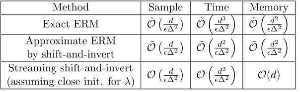
Table 1: Summary of sample, time (measured in floating point operations), and memory complexities of different approaches, in terms of (d, ∆, ), for stochastic CCA with Gaussian inputs. We give the dominant term in complexities as→0. Note that the time complexity of exact ERM is dominated by forming the eigen-system, while the memory complexity of ERM is dominated by saving the dataset.

Method Sample Time Memory

Exact ERM O˜ d ∆2

_˜

O d3 ∆2

˜

O d2 ∆2

Approximate ERM

by shift-and-invert O˜ d ∆2

_˜

O_∆d22

˜

O_∆d22

Streaming shift-and-invert (assuming close init. forλ) O

d ∆2

O d2 ∆2

O(d)

Lemma 19 (Lower bound for single canonical pair model) Suppose the data is gen-erated by the single canonical pair model. Let (u,v) be some estimate of the canonical directions (u∗,v∗) based on N samples. Then, there is a universal constant C, so that for

N sufficiently large, we have:

inf

u,v _usup∗_,v∗∈

F(dx,dy,∆)

E[1−align((uT,vT); (u∗,v∗))]≥C

d

∆2_N.

This lemma implies that, to estimate the canonical directions up to -suboptimality in our measure of alignment, we expect to use at leastO d

∆2

samples. We therefore observe that, for Gaussian inputs, the sample complexity of the our streaming algorithm matches that of the minimax rate of CCA, up to small factors.

In Table 1, we collect the complexities of different approaches, namely exact optimization of ERM (Section 3), stochastic optimization of ERM with shift-and-invert (Section 4), and streaming shift-and-invert (Section 5). We observe that while all three approaches are sample efficient (up to small factors), stochastic and streaming algorithms are more efficient in time and memory.

6. Conclusion

In this paper, we have studied the sample complexity of population CCA for several classes of input distributions, and proposed sample-efficient algorithms for learning the first pair of canonical directions. While the original problem is nonconvex, we exploit its structure as an eigenvalue problem, and analyze the statistical performance of the shift-and-invert power iterations.

(i.e., Exx = Eyy =I) and y being one-hot representations for class labels respectively. It is an interesting question if our general approach can be adapted to study the statistical performance of the kernel extension of CCA (Fukumizu et al., 2007).

Acknowledgement

Research partially supported by NSF BIGDATA award 1546462.

References

Zeyuan Allen-Zhu and Yuanzhi Li. LazySVD: Even faster SVD decomposition yet without agonizing pain. In Advances in Neural Information Processing Systems, 2016.

Zeyuan Allen-Zhu and Yuanzhi Li. Doubly accelerated methods for faster CCA and general-ized eigendecomposition. In Proc. of the International Conference on Machine Learning, 2017.

Raman Arora, Andy Cotter, Karen Livescu, and Nati Srebro. Stochastic optimization for PCA and PLS. In 50th Annual Allerton Conference on Communication, Control, and Computing, 2012.

Raman Arora, Teodor V. Marinov, Poorya Mianjy, and Nathan Srebro. Stochastic approx-imation for canonical correlation analysis. InAdvances in Neural Information Processing Systems, 2017.

Sanjeev Arora, Satish Rao, and Umesh Vazirani. Expander flows, geometric embeddings and graph partitioning. Journal of the ACM, (2), 2009.

Francis R. Bach and Michael I. Jordan. A probabilistic interpretation of canonical correla-tion analysis. Technical Report 688, Department of Statistics, University of California, Berkeley, April 21 2005.

Marcus Carlsson. Perturbation theory for the matrix square root and matrix modulus. arXiv:1810.01464 [math.FA], October 2 2018.

Mengjie Chen, Chao Gao, Zhao Ren, and Harrison H. Zhou. Sparse CCA via precision adjusted iterative thresholding. arXiv:1311.6186 [math.ST], November 24 2013.

Zhehui Chen, Lin F. Yang, Chris J. Li, and Tuo Zhao. Dropping convexity for more efficient and scalable online multiview learning. InProc. of the International Conference on Machine Learning, 2017.

Chandler Davis and W. M. Kahan. The rotation of eigenvectors by a perturbation III.

SIAM Journal of Numerical Analysis, 7(1):1–46, 1970.

Kenji Fukumizu, Francis R. Bach, and Arthur Gretton. Statistical consistency of kernel canonical correlation analysis. Journal of Machine Learning Research, 8:361–383, Febru-ary 2007.

Chao Gao, Zongming Ma, and Harrison H. Zhou. Sparse CCA: Adaptive estimation and computational barriers. Annals of Statistics, 45(5):2074–2101, 2017.

Dan Garber and Elad Hazan. Fast and simple PCA via convex optimization. arXiv:1509.05647 [math.OC], November25 2015.

Dan Garber, Elad Hazan, Chi Jin, Sham M. Kakade, Cameron Musco, Praneeth Netrapalli, and Aaron Sidford. Faster eigenvector computation via shift-and-invert preconditioning. In Proc. of the International Conference on Machine Learning, 2016.

Rong Ge, Chi Jin, Sham M. Kakade, Praneeth Netrapalli, and Aaron Sidford. Efficient algorithms for large-scale generalized eigenvector computation and canonical correlation analysis. In Proc. of the International Conference on Machine Learning, 2016.

Eckart Gekeler. On the pointwise matrix product and the mean value theorem. Linear Algebra and its Applications, 35:183–191, 1981.

Gene H. Golub and Charles F. van Loan. Matrix Computations. Johns Hopkins University Press, 1996.

Roger A. Horn and Charles R. Johnson. Matrix Analysis. Cambridge University Press, 1986.

Roger A. Horn and Charles R. Johnson. Topics in Matrix Analysis. Cambridge University Press, 1991.

Harold Hotelling. Relations between two sets of variates. Biometrika, 28(3/4):321–377, 1936.

Daniel Hsu, Sham Kakade, and Tong Zhang. A tail inequality for quadratic forms of subgaussian random vectors. Electron. Commun. Probab., 17(52):1–6, 2012.

Rie Johnson and Tong Zhang. Accelerating stochastic gradient descent using predictive variance reduction. In Advances in Neural Information Processing Systems, 2013.

Hongzhou Lin, Julien Mairal, and Zaid Harchaoui. A universal catalyst for first-order optimization. In Advances in Neural Information Processing Systems, 2015.

Yichao Lu and Dean P. Foster. Large scale canonical correlation analysis with iterative least squares. InAdvances in Neural Information Processing Systems, 2014.

Zhuang Ma, Yichao Lu, and Dean Foster. Finding linear structure in large datasets with scalable canonical correlation analysis. In Proc. of the International Conference on Ma-chine Learning, 2015.

Yousef Saad. Numerical Methods for Large Eigenvalue Problems. Manchester University Press, 1992.

Nikhil Srivastava and Roman Vershynin. Covariance estimation for distributions with 2 +ε -moments. Annals of Probability, 41(5):3081–3111, 2013.

Roman Vershynin. Compressed Sensing: Theory and Applications, chapter Introduction to the Non-asymptotic Analysis of Random Matrices. Cambridge University Press, 2012.

Weiran Wang and Karen Livescu. Large-scale approximate kernel canonical correlation analysis. In Proc. of the International Conference on Learning Representations, 2016.

Weiran Wang, Jialei Wang, Dan Garber, and Nathan Srebro. Globally convergent stochas-tic optimization for canonical correlation analysis. In Advances in Neural Information Processing Systems, 2016.

Lin Xiao and Tong Zhang. A proximal stochastic gradient method with progressive variance reduction. SIAM Journal on Optimization, 24(4):2057–2075, 2014.

Appendix A. Auxiliary Lemmas

Lemma 20 The population canonical correlation is bounded by 1, i.e.,

ρ1 =σ1(T)≤1.

Proof By the Cauchy-Schwarz inequality of random variables, we have

ρ1 =E[(u∗>x)(v∗>y)]≤

q

E[(u∗>x)2]·

q

E[(v∗>y)2] =

p

u∗>Exxu· q

v∗>Eyyv= 1.

Lemma 21 (Distance between normalized vectors) For two nonzero vectors a,b ∈

Rd, we have

a kak −

b kbk

≤2ka−bk

kak .

Proof By direct calculation, we have

a kak −

b kbk

≤

a kak −

b kak

+

b kak −

b kbk

= ka−bk

kak +kbk ·

|kak − kbk| kak kbk

≤ ka−bk kak +

ka−bk kak

= 2ka−bk

where we have used the triangle inequality in the two inequalities.

Lemma 22 (Conversion from joint alignment to separate alignment) Letη∈ 0,1₄. Consider the four nonzero vectors a,x∈_Rdx _{and b,y∈}

Rdy such thatkak=kbk= 1. If

1

√

2·

a>x+b>y q

kxk2+kyk2

≥1−η, (18)

we also have

1 2

a>x kxk

+

b>y kyk

≥1−4η.

Proof By the Cauchy-Schwarz inequality, we have

a>x+b>y q

kxk2+kyk2

= a

>_x

kxk ·

kxk q

kxk2+kyk2

+b

>_y

kyk ·

kyk q

kxk2+kyk2 ≤

s

a>_x

kxk 2

+

b>_y

kyk 2

.

Thus according to (18), we obtain

a>x

kxk 2

+

b>y

kyk 2

≥2(1−η)2≥2−4η.

Since b_k>_yky2 ≤1, this implies

a>x kxk

≥p

1−4η≥1−4η

where the last step is due to the fact that √x ≥ x for x ∈ (0,1). Similarly we have

b>_y

kyk

≥1−4η. Then the theorem follows.

Lemma 23 (Moment inequalities of sub-Gaussian and regular polynomial-tail random vectors)Let z∈Rdbe isotropic and sub-Gaussian or regular polynomial-tail (see

their definitions in Lemma 3). Then for some constantC0 >0, we have

Ekzk2 ≤d, Ekzk4≤C0d2, E

q

>

z 4

≤C0

Proof Sub-Gaussian case The first bound is byEkzk2 =Etr zz> = tr (I) =d. To

prove the second one, note that according to Theorem 2.1 in Hsu et al. (2012), we have

P

kzk2 > C1(d+t)

< e−t

for all t >0. Therefore

Ekzk4 =

Z ∞

0

P

kzk4> sds

=

Z C₁2d2

0

P

kzk4 > s

ds+

Z ∞

C2 1d2

P

kzk4 > s

ds

≤C₁2d2+

Z ∞

C2 1d2

exp

−

√

s C1

−d

ds

≤C0d2.

Lastly,

E

q

>

z 4

=

Z ∞

0

P

q

>

z 4

> s

ds

≤ Z ∞

0

e−C

√

s_ds

≤C0.

Regular polynomial-tail case The first bound is still by Ekzk2 = Etr zz> =

tr (I) =d. When r >1, we have

Ekzk4 =

Z ∞

0

P

kzk4> sds

≤ Z C2d2

0

P

kzk4 > s

ds+

Z ∞

C2_d2P

kzk4 > s

ds

≤C2d2+

Z ∞

C2_d2

Cs−1+2rds

≤C0d2.

To prove the last bound, takeV=qq> in the definition of regular polynomial-tail random vectors, and then

P

q

>_z 2

> t

≤Ct−1−r,

for any t > C. We have

E

q

>

z 4

=

Z ∞

0

P

q

>

z 4

> s

ds

≤ Z C2

0

P

q

>

z 4

> s

ds+

Z ∞

C2 P

q

>

z 4

> s

ds

≤C2+

Z ∞

C2

Cs−1+2rds

Appendix B. Proofs for Section 1

B.1. Proof of Lemma 1

Proof Using the fact that u>Exxu∗ E 1 2 xxu

and v>Eyyv∗ E 1 2 yyv

are at most 1, the condition on alignment

implies

u>Exxu∗ E 1 2 xxu

=a>₁ E 1 2 xxu E 1 2 xxu

≥1−η

4,

v>Eyyv∗ E 1 2 yyv

=b>₁ E 1 2 yyv E 1 2 yyv

≥1−η

4.

Since {ai}ri=1 and {bi}ri=1 are orthonormal, we have

r X i=2    

a>_i E 1 2 xxu E 1 2 xxu     2

≤1−1−η

4 2 ≤ η 2, r X i=2    

b>_i E 1 2 yyv E 1 2 yyv     2

≤1−1−η

4

2 ≤ η

2.

Observe that

u>Exyv p

u>_E

xxu p

v>_E

yyv = (E

1 2

xxu)>T(E 1 2 yyv) E 1 2 xxu E 1 2 yyv = d X i=1 ρi    

a>_i E 1 2 xxu E 1 2 xxu        

b>_i E 1 2 yyv E 1 2 yyv    

≥ρ1 

  

a>_i E 1 2 xxu E 1 2 xxu        

b>₁ E 1 2 yyv E 1 2 yyv    

−ρ2 v u u u u u t r X i=2    

a>_i E 1 2 xxu E 1 2 xxu    

2vu u u u u t r X i=2    

b>_i E 1 2 yyv E 1 2 yyv     2

≥ρ1

1−η

4

2 −ρ1·

η

2 ≥ρ1(1−η)

where we have used the Cauchy-Schwarz inequality in the first inequality.

Appendix C. Proofs for Section 3

C.1. Proof of Lemma 3

sizenis large enough (as specified in the lemma), we have 1 N N X i=1

ziz>_i −I ≤ ν 2

with high probability for the sub-Gaussian class (Vershynin, 2012) and for the regular polynomial-tail class (Srivastava and Vershynin, 2013), givenN > C0_νd2 andN ≥C

0 d

ν2(1+r−1) respectively.

We then turn to bounding the error in each covariance matrix. We note that the

covariance of f :=

" E− 1 2 xx x E− 1 2 yy y #

is Ξ =

I T T> I

with kΞk = 1 +ρ1 ≤ 2 (since the eigenvalues ofΞare of the form 1±σi(T)). On the other hand, define

Φ:=

Exx

Eyy −1₂

Exx Exy E>_xy Eyy

1₂

satisfying ΦΦ>=Ξ

and we have f = Φz by the definition ofz. Furthermore, fi = Φzi,i = 1, . . . , N are i.i.d. samples of f. Therefore, it holds that

" 1 N PN i=1E −1 2

xx xix>i E

−1 2

xx −I _N1 PNi=1E

−1 2

xx xiy>i E

−1 2 yy −T 1

N PN

i=1E

−1₂

yy yix>i E

−1₂

xx −T> _N1 PNi=1E

−1₂

yy yiy>i E

−1₂

yy −I # = 1 N N X i=1

fif_i>−Ξ = Φ 1 N N X i=1

ziz>_i −I ! Φ> ≤ ΦΦ > · 1 N N X i=1

ziz>_i −I

=kΞk · 1 N N X i=1

ziz>_i −I ≤ν.

Since the norm of each block is bounded by the norm of the entire matrix, we conclude that the error in estimating each covariance matrix is bounded byν, as required by Proposition 2.

Remark 24 In view of Lemma 23 and the proof technique here, for the sub-Gaussian/regular polynomial-tail cases, the bound of kzk2 leads to a bound for kxk2 and kyk2:

E(kxk2+kyk2)≤ kExxk ·E

E− 1 2 xx x 2

+kEyyk ·E

E− 1 2 yy y 2

≤Ekfk2 ≤2Ekzk2≤Cd

for some constant C >0, where we have used Assumption 1 in the second inequality. And similarly, we have

E(kxk2+kyk2)2≤Ekfk4 ≤4Ekzk4≤C0d2

for some constant C0 >0.

Bounded case Consider the joint covariance matrix

Exx Exy E>_xy Eyy

which has eigenvalue bounded by 2 due to the assumption that kxk2+kyk2 ≤2. Apply-ing Vershynin (2012, Corollary 5.52), we obtain that

Σxx Σxy Σ>_xy Σyy

−

Exx Exy E>_xy Eyy

≤ν0 (19)

with probability at least 1−d−t2 whenN ≥C(t/ν0)2logdfor some constantC >0. Setting the failure probability δ = d−t2 gives t2 = log

1

δ

logd, and thus we require N ≥ C 1

ν02 log1_δ for 1−δ success probability.

Due to the block structure of the joint covariance matrix, (19) implies

kΣxy−Exyk ≤ν0, kΣxx−Exxk ≤ν0, kΣyy−Eyyk ≤ν0

hold simultaneously.

Now, to satisfy the first inequality of (9), observe that

E− 1 2 xx ΣxxE

−1 2 xx −I

=

E− 1 2

xx (Σxx−Exx)E

−1 2 xx

≤

E− 1 2 xx

· kΣxx−Exxk ·

E− 1 2 xx

≤ kΣxx−Exxk/γ

where we have used the assumption that σmin(Exx) ≥γ in the last inequality. Therefore, we obtain

E− 1 2 xx ΣxxE

−1₂

xx −I

≤ ν by setting ν0 = γν in (19), and this yields the N0(ν) chosen in the lemma. The other two inequalities of (9) can be obtained analogously.

C.2. Proof of Lemma 5

Proof This result can be derived from the main result of Mathias (1997) with a bit of detective work, which is needed to understand the higher order error term. As in Mathias (1997), assume without loss of generality that H = diag (λ1, . . . , λd) is diagonal. In the proof of Theorem 2, Mathias (1997) applied the Daleckii-Krein formula in his equation (4) with the O-notation, which can be rephrased as (see also Carlsson (2018)[Theorem 2.1]): forζ in a neighborhood of 0, it holds

ε:=

(H+ζΘ)12 −H 1 2 −ζ





λ

1 2 i λ

1 2 j

λ

1 2 i +λ

1 2 j



 d

i,j=1

◦(H−12ΘH− 1 2)

=O(ζ2)

where◦ denotes elementwise (Hadamard) multiplication.

and Johnson, 1991, Theorem 6.6.30 and page 549) to obtain:

ε≤ζ 2 2 τmax∈[0,ζ]

U(τ)

d X

k=1 "

1

p

λi(τ) + p

λj(τ)

·_p 1

λi(τ) + p

λk(τ)

·_p 1

λj(τ) + p

λk(τ) #d

i,j=1

◦hck(τ)c>_k(τ)

i U(τ)>

(20)

where H+τΘ=U(τ)·diag (λ1(τ), . . . , λd(τ))·U(τ)> is the eigenvalue decomposition of the perturbation of H, andck(τ) is thek-th column of X(τ) =U(τ)>ΘU(τ).

Define Z(τ) =

1 √

λi(τ)+

√ λj(τ)

d

i,j=1

. The summation enclosed in () of the right hand

side of (20) can be written as Z(τ)◦(Z(τ)◦X(τ))2. Thus continuing from (20) yields

ε≤ ζ

2

2 ·τmax∈[0,ζ]

Z(τ)◦(Z(τ)◦X(τ))2 .

On the one hand, by the assumption that kHk ≤σmax, we have kX(τ)k=kΘk=

H

1 2(H−

1 2ΘH−

1 2)H

1 2

≤ kHk · H

−1 2ΘH−

1 2

≤σmax. (21)

On the other hand, the matrixZ(τ) is positive semidefinite (see Horn and Johnson, 1991, Problem 9, page 348). Using the fact thatkA◦Bk ≤(maxiAii)· kBk for positive semidef-initeA and Hermitian B(Horn and Johnson, 1991, Theorem 5.5.18), we conclude

ε≤ ζ

2_σ2 max 2

"

max τ∈[0,ζ]maxi

1 2pλi(τ)

#3

.

Let ζ ≤ 3 4σ

−1

maxσmin. Then in view of (21) and the Weyl’s inequality, λi(τ) ≥ σmin₄ for all

τ ∈[0, ζ], and we have ε≤ 1 2ζ

2_σ2 maxσ

−3 2 min.

To sum up, we have shown so far the following first order approximation: for certain error matrixE ∈_Rd×d_{, it holds}

(H+ζΘ)12 =H 1 2 +ζ





λ

1 2 i λ

1 2 j

λ

1 2 i +λ

1 2 j



 d

i,j=1

◦(H−12ΘH− 1

2) +E where kEk ≤ 1 2ζ

2_σ2 maxσ

−3 2 min. Consequently, we have

(H+ζΘ)12H− 1

2 −I=ζ 



λ

1 2 i

λ

1 2 i +λ

1 2 j



 d

i,j=1

◦(H−12ΘH− 1

2) +EH− 1 2.

Mathias (1997) showed that the norm of the first term on the right hand size is of the order

O(logd·ζ). Combining this with the fact that

EH

−1 2 ≤

1 2ζ

2_σ2

maxσmin−2, we conclude that

EH

−1 2

=O(ζ) for ζ =O(σ

−2

C.3. Proof of Lemma 6

Proof In view of the Weyl’s inequality, we have

|ρ_b1−ρ1| ≤ Tb −T

= Σ− 1 2 xx ΣxyΣ

−1 2 yy −E

−1 2 xxExyE

−1 2 yy . (22)

For the right hand side of (22), we have the following decomposition

Σ− 1 2 xxΣxyΣ

−1 2 yy −E

−1 2 xx ExyE

−1 2 yy = Σ− 1 2 xx −E

−1 2 xx

ΣxyΣ

−1 2 yy +E

−1 2

xx (Σxy−Exy)Σ

−1 2 yy +E

−1 2 xx Exy

Σ−

1 2 yy −E

−1 2 yy

. (23)

By the equality

A−12 −B− 1 2 =B−

1 2

B12 −A 1 2

A−12,

the first term of the RHS of (23) becomes

Σ−

1 2 xx −E

−1 2 xx ΣxyΣ− 1 2 yy =E

−1 2 xx E 1 2 xx−Σ

1 2 xx Σ− 1 2 xx ΣxyΣ −1 2 yy . When E− 1 2 xx ΣxxE −1 2 xx −I

≤ν, according to Lemma 5, we have (by making the identification

thatH=Exx,ζ =

E− 1 2

xx(Σxx−Exx)E

−1 2 xx

, andΘ= (Σxx−Exx)/

E− 1 2

xx (Σxx−Exx)E

−1 2 xx ) E− 1 2 xx E 1 2 xx−Σ

1 2 xx

≤Cd·ν

forν ≤ 3 4γ

2_{. Combining with the fact that} Σ− 1 2 xx ΣxyΣ

−1 2 yy

≤1, we have

Σ− 1 2 xx −E

−1 2 xx

ΣxyΣ− 1 2 yy

≤Cd·ν.

A similar bound can be obtained for the third term of (23). Observe that when

E− 1 2 yy ΣyyE

−1 2 yy −I

≤

ν < 1, we have kΣyy−Eyyk ≤ ν and all eigenvalues of Σyy lie in [γ −ν,1 +ν].

Addi-tionally, E− 1 2 yy ΣyyE

−1₂

yy is invertible, and all eigenvalues of Σ

−1₂

yy EyyΣ

−1₂

yy lie in [_1+ν1 ,₁−1ν], impling that Σ− 1 2 yy EyyΣ

−1₂

yy −I

≤ ₁₋ν_ν. According to Lemma 5, we have (by mak-ing the identification that H = Σyy, ζ =

Σ− 1 2

yy (Σyy−Eyy)Σ

−1 2 yy

, and Θ = (Σyy −

Eyy)/ Σ− 1 2

yy (Σyy−Eyy)Σ

−1 2 yy ) E 1 2 yy−Σ

1 2 yy Σ− 1 2 yy

≤ Cd·ν

forν ≤ 3₄γ_1+ν−ν2, which is satisfied for ν ≤ 1₄γ2. Therefore, we can bound the third term of (23) as

E− 1 2 xx Exy Σ− 1 2 yy −E

−1₂

yy = E− 1 2 xx ExyE

−1₂

yy

E 1 2 yy−Σ

1 2 yy Σ− 1 2 yy ≤ E− 1 2 xx ExyE

−1 2 yy · E 1 2 yy−Σ

1 2 yy Σ− 1 2 yy

≤ Cd·ν

1−ν ≤2Cd·ν

where we have used the fact that

E− 1 2 xx ExyE

−1₂

yy

≤1 by Lemma 20.

For the second term of (23), we have by assumption that

E− 1 2

xx (Σxy−Exy)Σ

−1₂

yy ≤ν.

Applying the triangle inequality, we obtain from (23) that

Σ− 1 2 xx ΣxyΣ

−1 2 yy −E

−1 2 xx ExyE

−1 2 yy

≤4Cd·ν. (25)

To sum up, it suffices to set ν = _4C0

d to ensure

Tb −T

≤

0_{, and this yields the desired}

sample complexity.

C.4. Proof of Theorem 9 Proof Apply Lemma 6 with0 =

√

∆

4 where∈(0,1) is the desired accuracy in Theorem 9. Since

T−Tˆ

≤

0 _< ∆

4, the eigenvalues of ˆT are within ∆

4 of those of T due to Weyl’s inequality, so there exists a positive singular gap of ∆₂ for the empirical estimate ˆT, whose first pair of singular vectors is unique. In view of the off-diagonal structure ofCb, we observe

that C− ˆ C = T− ˆ T ≤

0 _{and that the top eigenvector of ˆC is unique. Then with}

the number of samples given in the theorem ensuring the 0 perturbation, according to the Davis-Kahan sinθ theorem (Davis and Kahan, 1970), the top eigenvectors ofCand Cb are

well aligned:

sin2θ≤ C−Cb

2 ∆2 ≤

02

∆2 =

16 (26)

whereθ is the angle between the top eigenvector ofCand that of Cb. This is equivalent to

E 1 2

xxu∗−Σ 1 2 xxbu

2 + E 1 2

yyv∗−Σ 1 2 yyvb

and so max E 1 2

xxu∗−Σ 1 2 xxbu

2 , E 1 2

yyv∗−Σ 1 2 yybv

2! ≤ ₈.

In the rest of the proof, we fix the issue of incorrect normalization of (ub,bv). Recall we

have shown in the proof of Lemma 6 that (see e.g., (24))

I−E 1 2 xxΣ− 1 2 xx

≤0 ≤ √

4 .

Consequently, we have

E 1 2

xxu∗−E 1 2 xxub

2 = E 1 2 xxu∗−

E 1 2 xxΣ− 1 2 xx Σ 1 2 xxbu

2 ≤ E 1 2

xxu∗−Σ 1 2 xxub

+

I−E 1 2 xxΣ− 1 2 xx Σ 1 2 xxub

2 ≤2 E 1 2

xxu∗−Σ 1 2 xxub

2 + 2

I−E 1 2 xxΣ− 1 2 xx 2 ≤ 4 + 8 ≤ 2

where we have used the facts that (x+y)2 ≤ 2x2 + 2y2 and

Σ 1 2 xxbu

= 1 in the second

inequality.

According to Lemma 21, we then have

E 1 2 xxu∗ E 1 2 xxu∗ − E 1 2 xxub E 1 2 xxub

2 ≤ 4 E 1 2

xxu∗−E 1 2 xxub

2 E 1 2 xxu∗

2 = 4

E 1 2

xxu∗−E 1 2 xxub

2 ≤2

and thus the alignment between these two vectors is

b

u>Exxu∗ E 1 2 xxbu

= 1−1

2 E 1 2 xxu∗ E 1 2 xxu∗ − E 1 2 xxbu E 1 2 xxbu

2

≥1−.

A similar bound is obtained for vb:

b

v>Eyyv∗ E 1 2 yybv

≥1−.

Averaging the above two inequalities yields the desired result. Requiring that0 =

√

∆ 4 ≤

Cdγ2 as in Corollary 7 leads to the extra condition that≤ 16C2

dγ4