Redundancy Allocation Combined with Supplier Selection for Design of Series-parallel Systems

(1)

Please cite this article as: R. Soltani, A. A. Tofigh, S. J. Sadjadi, Redundancy Allocation Combined with Supplier Selection for Design of Series-parallel Systems,International Journal of Engineering (IJE), TRANSACTIONS B: Applications Vol. 28, No. 5, (May 2015) 730-737

International Journal of Engineering

J o u r n a l H o m e p a g e : w w w . i j e . i r

Redundancy Allocation Combined with Supplier Selection for Design of

Series-parallel Systems

R. Soltania_{*, A. A. Tofigh}b_{, S. J. Sadjadi}c

a_{Department of Industrial Engineering, Science and Research Branch, Islamic Azad University, Tehran, Iran} b _{Department of Industrial Engineering, Amir Kabir University of Technology, Tehran, Iran}

c _{Department of Industrial Engineering, Iran University of Science and Technology, Tehran, Iran}

P A P E R I N F O

Paper history: Received 24 June 2014

Received in revised form 10November 2014 Accepted 18December 2014

Keywords: System Design Redundancy Allocation Supplier Selection Price Discounting Warranty Length Compromise Programming

A B S T R A C T

Designing highly reliable and economical systems is of interest in today’s competitive world. In this paper, enhancing system reliability through redundancy allocation is investigated, where the supplier selection is taken into account and redundant components are provided from appropriate suppliers with the most suitable offers such as discount on purchasing price of components, warranty length of components, things like that, so that the system reliability, profit and the warranty length proposed by suppliers are simultaneously maximized. The resulting multi-objective model is then solved with the well-known compromise programming approach and the performance of the proposed approach is investigated through a numerical example.

doi: 10.5829/idosi.ije.2015.28.05b.11

1. INTRODUCTION1

System designers employ some techniques to enhance the system’s reliability to assure its function for a specific period of time under defined circumstances. One way to increase the system reliability is the allocation of redundant components in parallel. Many scholars have studied the redundancy allocation problem (RAP) with different assumptions. Soltani [1] presented a comprehensive review on reliability optimization problems, in particular, RAP. In the following sections the focus is on the models proposed in this area and less attention is paid to the solution approaches.

In the field of active strategy and binary state of components, Fyffe et al. [2] are the first who proposed a model for RAP where system’s reliability is maximized subject to constraints on cost and weight. Ramirez-Marquez et al. [3] modeled RAP using max-min approach, where the reliability of the subsystem with minimum reliability is maximized subject to constraints

1_{*Corresponding Author}_’_{s Email:} _{roya.soltani@gmail.com (R.}

Soltani)

on cost and weight. Sun and Ruan[4] formulated RAP such that system’s cost is minimized subject to the requirement of satisfying the minimum system’s reliability. They presented an exact algorithm to solve the model. Coit, and Konak [5] considered a multi-objective RAP where the reliabilities of subsystems are maximized, simultaneously subject to constraints on cost and weight. They presented a multiple weighted objectives heuristic to solve the model. Salazar et al. [6] studied three types of reliability optimization problems including redundancy allocation, reliability allocation and reliability-redundancy allocation. Their proposed multi-objective RAP maximizes system’s reliability while minimizing system’s cost, and they solve it through NSGAII. Taboada et al. [7] considered a multi-objective model, which maximizes system’s reliability while minimizing system’s cost and weight, and they solve it using NSGA. Taboada et al. [8] proposed a multiple objective evolutionary algorithm to solve a multi-objective redundancy allocation problem where the objectives are maximizing system’s reliability and minimizing system’s cost and weight. Wang et al. [9] considered a multi-objective RAP to maximize system’s

(2)

reliability and minimize system’s cost with nonlinear cost and weight and solved the resulting model using NSGAII. Mahapatra [10] presented a bi-objective model, which simultaneously maximizes the system’s reliability and entropy considering nonlinear cost constraint. They solved the resulted model using global criterion method. Soylu and Ulusoy [11] considered the problem of maximizing the minimum subsystem reliability while minimizing the overall system cost and found the Pareto solutions of this problem by the augmented epsilon-constraint approach for small and moderate sized instances. Then, they applied a well-known sorting procedure, UTADIS, to categorize the solutions into preference ordered classes. Khalili-Damghani and Amiri [12] considered an existing multi-objective RAP which involves maximizing system’s reliability and minimizing system’s cost and weight, and solved it through a method based on epsilon-constraint and data envelopment analysis. Soltani et al. [13] studied RAP with discount consideration and presented heuristic and meta-heuristic approaches to deal with the problem. For further study on heuristic and meta-heuristic approaches for RAP with active strategy, readers are referred to the works by Sadjadi and Soltani [14, 15]. Recently, they [16] presented a robust possibilitic programming approach and developed robust models for RAP with active strategy.

In the area of RAP with cold standby strategy, Coit [17] studied cold standby redundancy optimization for non-repairable systems and developed a zero-one linear programming model to solve the problem. Coit [18] studied the same redundancy allocation problem where there are redundancy strategy choices for subsystems. Tavakkoli-Moghaddam et al. [19] developed a genetic algorithm to solve the same problem proposed by Zeleny and Cochrane [20]. Bi or multi-objective versions of the mentioned problem have been studied by some authors [21, 22] independently considered a bi-objective model for RAP to optimize reliability and cost of the system with choice of redundancy strategy and solved the resulting model through NSGAII. Azizmohammadi et al. [23] considered a multi-objective RAP where the system reliability is maximized while minimizing the system’s cost and volume. They proposed a hybrid multi-objective imperialist competition algorithm to solve the model. Soltani et al. [13] considered a multi-objective RAP with the choice of a redundancy strategy and reliability, cost and weight as objective functions. Soltani et al. [24] RAP with the choice of a redundancy strategy. They considered reliability, cost and entropy as objective functions and solved the problem by a compromise programming approach. They [25] presented an interval programming approach for RAP with the choice of a redundancy strategy. In other literatures [26-28][27] have considered RAP respectively with active, cold standby and choice of redundancy strategy with interval uncertainty of

components and formulated the model through Min-Max regret approach to deal with uncertainty. Feizollahi et al. [29, 30] studied RAP with respectively active and cold standby strategies with budgeted uncertainty for components reliabilities. The above-mentioned works do not consider the suppliers and their offers such as discount on price and other services such as warranty services in the system design. In this paper, a new multi-objective model for RAP is proposed in which the discount on buying price and warranty length are taken into consideration such that system reliability, profit and warranty length offered by suppliers are simultaneously maximized. In addition, the mathematical compromise programming approach is implemented to find the Pareto points of the proposed multi-objective model. The rest of the paper is organized as follows. In section 2, the problem is described and the proposed

mathematical model presented. Compromise

programming technique as a solution procedure is presented in section 3. Experimental results are presented in section 4. Finally, conclusion is presented in section 5 along with some future research directions.

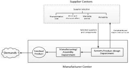
2. PROBLEM DESCRIPTION AND FORMULATION

(3)

arrangement of the components leads to a reliable design. In supplier centers, suppliers are selected based on some criteria such as price and discount offers, reliability of components, warranty periods and transportation cost. After the design phase, the system is produced in the manufacturing/assembly department and the final product is ready for release to the market. In customer zones, there is a demand for the system/product which depends on the potential market size and the selling price. Therefore, the designer needs to look ahead and make a tradeoff between the system reliability, system profit and warranty length of the system. These objectives are met by solving the proposed multi-objective model of this paper. Examples of such a model can be found in areas such as electrical and electronic, telecommunication, manufacturing industries, etc., where different components are provided from suitable suppliers to make systems. Assumptions:

· The system/product has series-parallel structure.

· The redundancy strategy is active.

· The components are in two states, i.e. binary states.

· The discount policy offered by suppliers is all unit discount policy.

· Production value equals to demands.

· A single product is produced.

· The capacity of suppliers is unlimited. Indices:

i: Set of subsystems j: Set of components k: Set of suppliers

q: Set of discount intervals Variables:

i

N

: The number of components required for subsystem i( ∈ ,∀ )

k i

X, : The number of components in all systems which

is required for subsystem i and purchased from supplier k( _, _∈ _∪_{{0} ,}_∀_, )

k i

Y, : A binary variable which is one if supplier k is

selected to provide components of subsystem i, and zero otherwise.

Figure 1. Conceptual model indicating the relation between system designer and suppliers

, : A binary variable which is one if discount interval q is selected for component of subsystem i, and zero otherwise. (∀ , = 1, … , )

P: Selling price for one system D: Demand of the system

Parameters:

max

n

: Maximum number of components in each

subsystem

b

: Potential market size

a

: Price elasticity of the demand k

i

w

_, ,

r

_i_,_k,

wr

_i_,_k: Weight, reliability and warranty associated with component i supplied from supplier k W: Available weight for each system

S: Number of subsystems K: Number of suppliers M: A big number

i

A

: Assembly cost of each component in subsystem i

tr

C

: Transportation cost per unit of products per unit distance

k

d

: Distance from supplier k to the manufacturer center

j i

n

_, : Discount breaking points

t

: Number of breaking points

k j i

C

_, _, : Purchasing price for each unit of the components required for subsystem

i

offered by supplier k that corresponds to the j-th discount breaking point (j = 1, 2, . . . , t)

k j,

g

: Discount factor in the j-thdiscount interval proposed by supplier k

Mathematical model:

Õ å

= = úû

ù ê ë é -´ -= S i K k N k i k

i r i

Y Z Max 1 1 , ,

1 1 (1 ) (M1)

åå

= = ´ = K k S i k i k i Y wr Z Max 1 1 , , 2

å

åå

å

= = = = = = ´ ´ -´ ´ + ´ -´ = S i k i K k k tr S i i i S i K k t j i j i k j i k i X d C D N A N C Y D P Z Max 1 , 1 1

1 1 1

, , , , 3 ) ) ( ( l S i Y K k k

i 1 1,..., 1 , = =

å

= (1-1) S i D X N K k k i

i , 1,...,

1 , ₌ =

å

= (1-2) W N w Y S i K

k ik ik i

£ ´ ´

åå

(4)

S … 1, = i , ) 1

( ,1

1

, i

i

i n M

N £ + -l (1-5)

) 1 ( _, ₁ 1

, ,

,j< i+ ij£ ij++ - ij+

i N M n M

n l l i=1,…,S ,

j= 1, …, t-2 (1-6)

å

-= - < +

1

1 , 1

,

t

k k i i

t

i N M

n l (1-7)

k i k

i

C

,1, = , ,

C

i,2,k =

g

1,k

C

i,k, ….,

k i k t k t

i

C

,,

=

g

-1, , ,i= 1,…,S , k=1,…,K

(1-8)

(1-9)

K k S i Y M

Xi,k£ ´ i,k , =1,..., =1,..., (1-10)

(1-11)

max

n

N

_i

£

, , i= 1,…,S (1-12)

K k

S i

Y_i,_kÎ{0,1} , =1,..., , =1,..., (1-13)

D Xik£

£ _,

0 ,i= 1,…,S , k= 1,…,K _(1-14)

∈ , = 1, … , (1-15)

, ∈ ∪{0} , = 1, … , , = 1, … , (1-16)

The first objective function maximizes the system reliability of the series-parallel system. The term

i

N k i

r )

1 (

1- - , calculates the reliability of each

subsystem. The summation

å

=

K

k ik

Y

1 ,

pertains to the

supplier selection. When

Y

_i_,_k is one, component i is provided from supplier k. The second objective function maximizes the warranty periods offered by suppliers. The third objective function maximizes the net profit resulting from selling the system with respect to purchasing cost of components, assembly costs and transportation costs. In the purchasing cost of components the discount offered by suppliers are considered. Constraint (1-1) states that just one supplier is selected for components of each subsystem i. Constraint (1-2) calculates the number of components required for subsystem i. Constraint (1-3) imposes a restriction on the weight of the system. Constraint (1-4) calculates the demand as a function of the potential market size and the price elasticity of the demand. Constraints (1-5) to (1-7) are defined to determine the discount interval for the quantity of buys. If the k-th discount interval is hold, the (k-1)-th discount interval reaches to its upper breaking point. Constraint set (1-8) defines the cost of component iin each discount interval k. Constraint set (1-9) states that only one discounting interval is considered for each subsystem. Constraint

(1-10) defines the relationship between

X

_i_,_k and

Y

_i_,_k. Constraint set (1-11) shows the binary nature of the variables considered for choosing a discount interval. Constraint set (1-12) provides an upper bound on the number of components in subsystemi. Constraint set (1-13) shows the binary nature of the variables used for selecting suppliers. Constraint set (1-14) defines an upper bound on the total quantity of purchasing of component i from supplier k.Constraint sets (1-15) and (1-16) define the integer natures of variables N and X.

3. COMPROMISE PROGRAMMING

Compromise programming is a mathematical

programming technique which was originally developed in references [20, 31]. This method can be used for optimization of multi-objective problems to obtain the optimal solution, and also for comparing the performance of alternatives in multi-criteria decision making analyses. As a matter of fact, the best compromise solution from a set of solutions is selected by a measure of distance called distance metric through which a discrete set of solutions is ranked according to their distance from an ideal solution. Mathematically, compromise programming distance metric is presented in Equation (1).

p n

i

p

i i

i i i

p _Z _Z

Z Z w w L

1

)

( _÷÷

ø ö ç

ç è æ

ú û ù ê

ë é

-=

å

= + -+

(1)

where n is the number of objectives, in this paper n=3, p is a parameter determining the norm of the Lp metric (

¥ Î1,2,

p ),

w

_ithe weight of the objective function i,

i

Zthe value of the objective function i, and +

i

Z and

-i Z the ideal and nadir values of the objective function i, respectively. For maximization problems, the former is achieved through maximizing each objective function subject to the constraints whilst the latter is determined by minimizing those objectives. This procedure is reversed for minimization problems.

The parameter p represents the importance of the maximal deviation from the ideal solution. If p=1, all deviations have equal importance. If p=2, the importance of deviations are in proportion to their magnitude. As p increases, the importance of the deviations also increases. Similarly,

w

_is are the weights for various deviations which identify the relative importance of each objective. Apparently, for different values of p in Lp metrics and

w

_i, different compromise

solutions can be obtained. For p = 1, the Lp metric, i.e.

L1, is called Manhattan metric. L2 is called the

Euclidean metric and

L

_¥is the Chebychev metric. In all

S i

t i i

i,1+l,2+...+l, =1 =1,K,

l

t j S i j

i, Î{0,1} =1,K, , =1,...,

(5)

cases, the corresponding metric needs to be minimized according to models M2, M3 and M4 for L1, L2 and

L

¥,

respectively.

-+ + -+ + -+ +

-+ -+

-3 3

3 3 3 2 2

2 2 2 1 1

1 1 1 min

Z Z

Z Z w Z Z

Z Z w

s.t.Constraints of model(M1)

(M2)

2

2 2

3 3

1 1 2 2

1 2 3

1 1 2 2 3 3

Z Z

Z Z Z Z

w w w

Z Z Z Z Z Z

min é_ê ₊+-_-_úù+ _êé +₊- _-_úù_{+ ê}é +₊-_-_úù

- -

-ë û ë û ë û

s.t.Constraints of model(M1)

(M3)

¥ -+ +

¥ -+

+ ¥

£ ú û ù ê

ë é

-£ ú û ù ê

ë é

-£ ú û ù ê

ë é

-D Z Z

Z Z w

D Z Z

Z Z w

D Z Z

Z Z w

t s

D

3 3

3 3 3

2 2

2 2 2

1 1

1 1 1

. . min

Constraints of model(M1)

(M4)

4. EXPERIMENTAL RESULTS

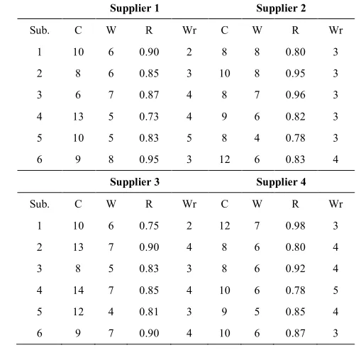
In this section, a numerical example is presented to show the performance of the proposed model and the corresponding solution approach. The designer aims at designing a system composed of 6 subsystems arranged in series. He/she wants to enhance the system reliability by making use of redundancy. There are 4 suppliers who can provide the required components. The suppliers present components with different reliability, weight and cost. They also offer discount on quantity of buys. The designer wants to select the suitable suppliers with respect to their offers and their transportation cost so that a highly reliable and economical system is designed. The input data are presented in Table 1.The price elasticity of the demand and the potential market size are assumed as -1.5 and 150000, respectively. The assembly costs of components in subsystems are 4, 6, 5, 5, 4, and 6, respectively. Distances from suppliers’ centers to manufacturer’s center are 10, 9, 10, and 9, respectively. All suppliers offer discount on price with three breaking points. The upper bounds of the first and second discount intervals are 2 and 3, respectively. The discount factors of the second and third intervals are0.95 and 0.9 for the first supplier, 0.9 and 0.85 for the second supplier, 0.95 and 0.85 for the third supplier and finally 0.85 and 0.8 for the fourth supplier, respectively. Transportation cost per unit of products per unit distance,

C

_tr , is assumed to be 5 unit of money. Maximum number of components in each subsystem is 4. Total allowed weight for each system is 150.

TABLE 1. Input data for components provided by suppliers (Sub: Subsystem; C: Purchasing Price; W: Weight; R: Reliability; Wr: Warranty Length)

Supplier 1 Supplier 2

Sub. C W R Wr C W R Wr

1 10 6 0.90 2 8 8 0.80 3

2 8 6 0.85 3 10 8 0.95 3

3 6 7 0.87 4 8 7 0.96 3

4 13 5 0.73 4 9 6 0.82 3

5 10 5 0.83 5 8 4 0.78 3

6 9 8 0.95 3 12 6 0.83 4

Supplier 3 Supplier 4

Sub. C W R Wr C W R Wr

1 10 6 0.75 2 12 7 0.98 3

2 13 7 0.90 4 8 6 0.80 4

3 8 5 0.83 3 8 6 0.92 4

4 14 7 0.85 4 10 6 0.78 5

5 12 4 0.81 3 9 5 0.85 4

6 9 7 0.90 4 10 6 0.87 3

TABLE 2. Ideal and Nadir solutions

Ideal point Nadir point

Objective 1(Reliability) 0.999 0.235

Objective 2(Warranty) 25 17

Objective 3 (Profit) 3077.405 0

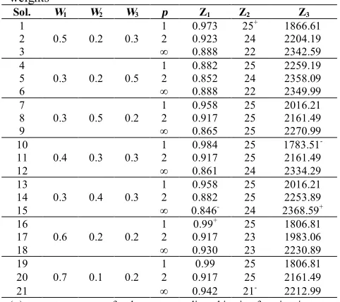
To start with compromise programming, ideal and nadir points need to be calculated. The ideal point is computed by maximizing each objective function separately. On the other hand, the nadir point is computed by minimizing each objective function separately in this study. All models are solved using GAMS (General Algebraic Modeling System) version 23.8.2 and the nadir and ideal points are presented in Table 2. By varying weights of the objectives and norms of the Lp metric the Pareto set is constructed. In this

paper, p=1, 2, ∞.

In fact, solving the proposed model using the compromise programming technique results in different Pareto solutions depending on the selected norm of the Lp metric and the weights of the objectives. Here, we

used 7 different settings of weight vectors and 3 norms of Lp given in Table 3a and Table 3b. Hence, we solved

(6)

determine the best solution of the set. There are four general classes of methods for determining the best solution in a Pareto set: no-preference, a posteriori, a priori, and interactive methods [32]. In no-preference approaches, which do not include the preferences of the decision maker, the best solution is defined by geometric relationships only. A common approach is to use the L2 norm [33, 34], where the best result is the

point form Pareto set that has the least geometric distance from the utopia point. Therefore, in this paper, we use L2 norm to decide about the best compromise

solution. Before deciding about the best compromise solution amongst non-dominated solutions, the objective functions are normalized through Equation (2).

n i x f x f

x f x f

i i

i

i _, ₁_,...,

) ( ) (

min max

min

= "

-(2)

where, _fmin(_x)

i and ( )

max x

fi are the minimum and

maximum values for fi(x)in the Pareto optimal set. The

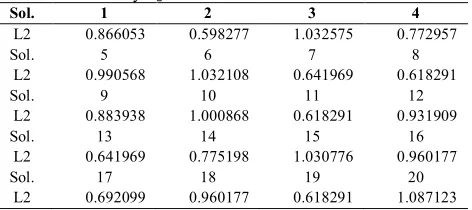
results for p=2 are shown in Table 4. The results show that solution 2 is the best compromise solution with the lowest L2 norm. The resulting solution indicates that in

order to design a highly reliable and economical system, redundancy levels should be set to 1, 2, 2, 3, 2, 2 and provided from suppliers 4, 3, 4, 4, 4, 3, respectively. Also, the price of the system is 1778.447 so that the profit, warranty and reliability are simultaneously maximized. The corresponding values for profit, reliability and warranty are 2204.193, 0.923 and 24, respectively.

The selected solution reveals that two suppliers are selected to provide the required components.

TABLE 3a. Experimental results with different Lp metrics and weights

Sol. W1 W2 W3 p Z1 Z2 Z3

1

0.5 0.2 0.3 1 0.973 25

+ _1866.61

2 2 0.923 24 2204.19

3 ∞ 0.888 22 2342.59

4

0.3 0.2 0.5

1 0.882 25 2259.19

5 2 0.852 24 2358.09

6 ∞ 0.888 22 2349.99

7

0.3 0.5 0.2

1 0.958 25 2016.21

8 2 0.917 25 2161.49

9 ∞ 0.865 25 2270.99

10

0.4 0.3 0.3

1 0.984 25 1783.51

-11 2 0.917 25 2161.49

12 ∞ 0.861 24 2334.29

13

0.3 0.4 0.3

1 0.958 25 2016.21

14 2 0.882 25 2253.89

15 ∞ 0.846- ₂₄ _2368.59+

16

0.6 0.2 0.2

1 0.99+ ₂₅ _1806.81

17 2 0.917 23 1983.06

18 ∞ 0.930 23 2230.89

19

0.7 0.1 0.2

1 0.99 25 1806.81

20 2 0.917 25 2161.49

21 ∞ 0.942 21- _2212.99

(+):presents _Zmax₍_x₎

i for the corresponding objective function i (-): presents _Zmin₍_x₎

i for the corresponding objective function i

TABLE 3b. Experimental results with different Lp metrics and weights (Dist.: Distance;N_i_,_k:number of components required for subsystem iin one system supplied from supplier k)

Sol. Dist. Solution

1 0.135 N1,4=2,N2,3=2,N3,4=4,N4,4=4,N5,1=3,N6,3=2

2 0.180 N,14=1,N2,3=2,N3,4=2,N4,4=3,N5,4=2,N6,3=2

3 0.075 N1,4=1,N2,2=2,N3,4=2,N4,4=2,N5,4=2,N6,4=2

4 0.179 N,14=1,N2,3=2,N3,4=2,N4,4=2,N5,1=2,N6,3=2

5 0.204 N1,4=1,N2,3=2,N3,2=,1N4,4=2,N5,1=2,N6,3=2

6 0.118 N1,4=1,N2,2=2,N3,4=2,N4,4=2,N5,4=2,N6,4=2

7 0.085 N,14=2,N2,3=2,N3,4=2,N4,4=,3N5,1=,3N6,3=2

8 0.146 N1,4=1,N2,3=2,N3,4=2,N4,4=3,N5,1=2,N6,3=2

9 0.053 N,14=1,N2,3=2,N3,4=2,N4,4=2,N5,1=2,N6,2=2

10 0.134 N1,4=2,N2,4=4,N3,4=2,N4,4=4,N5,1=3,N6,2=4

11 0.177 N1,4=1,N2,3=2,N3,4=2,N4,4=3,N5,1=2,N6,3=2

12 0.072 N1,4=1,N2,4=2,N3,4=2,N4,4=2,N5,3=2,N6,4=2

13 0.119 N1,4=2,N2,3=2,N3,4=2,N4,4=3,N5,1=3,N6,3=2

14 0.169 N1,4=1,N2,3=2,N3,4=2,N4,4=2,N5,1=2,N6,3=2

15 0.069 N1,4=1,N2,3=2,N3,4=2,N4,4=2,N5,1=2,N6,1=1

16 0.09 N1,4=2,N2,3=3,N3,4=3,N4,4=4,N5,1=3,N6,3=3

17 0.211 N1,3=3,N2,3=3,N3,4=2,N4,4=2,N5,4=3,N6,3=2

18 0.055 N1,4=1,N2,2=2,N3,4=2,N4,4=3,N5,3=2,N6,4=2

19 0.091 N1,4=2,N2,3=3,N3,4=3,N4,4=4,N5,1=3,N6,3=3

20 0.161 N1,4=1,N2,3=2,N3,4=2,N4,4=3,N5,1=2,N6,3=2

21 0.056 N1,4=1,N2,2=2,N3,2=2,N4,4=3,N5,4=2,N6,1=2

Figure 2. Pareto Solutions

This solution also has the less geometric distance from the ideal solution. In fact, the ideal solution is infeasible. But, through the compromise programming approach a tradeoff between objectives is made and a set of Pareto solutions based on their distance from the ideal solution is obtained.

0.8 0.85

0.9 0.95

1

1600 1800 2000 2200 2400

21 22 23 24 25

W

ar

ran

ty

(7)

TABLE 4. Choosing the best compromise solution from 20 Pareto solutions by L2 norm

Sol. 1 2 3 4

L2 0.866053 0.598277 1.032575 0.772957

Sol. 5 6 7 8

L2 0.990568 1.032108 0.641969 0.618291

Sol. 9 10 11 12

L2 0.883938 1.000868 0.618291 0.931909

Sol. 13 14 15 16

L2 0.641969 0.775198 1.030776 0.960177

Sol. 17 18 19 20

L2 0.692099 0.960177 0.618291 1.087123

However, in most cases, the decision makers want to decide based on a unique solution. Therefore, once again the proposed L2 norm is implemented to the

Pareto set and the nearest solution to the ideal solution is selected.

5. CONCLUSION

The redundancy allocation problem requires the appropriate selection of components that are usually provided by external suppliers. The components provided by suppliers might have different reliabilities, weights, costs, etc. This paper presents a multi-objective model, which for the first time considers the supplier selection in the redundancy allocation problem. The multi-objective model simultaneously maximizes the system reliability, profit and the warranty period offered by suppliers. The integration of the supplier selection process into the RAP might better represent the real life conditions. The resulting model is solved with the

compromise programming approach and its

performance is investigated through a numerical example. The solution selected by the compromise programming approach has the advantage that has the least geometric distance from the ideal solution and maximizes the three objectives, simultaneously. For future work on this study, heuristic and meta-heuristic approaches can be implemented to solve large scale problems. Furthermore, simplifying assumptions considered in this paper such as unlimited capacity for suppliers can be replaced with the capacity restriction to make the model more realistic.

6. REFERENCES

1. Soltani, R., "Reliability optimization of binary state non-repairable systems: A state of the art survey", International Journal of Industrial Engineering Computations, Vol. 5, No. 3, (2014), 339-364.

2. Fyffe, D.E., Hines, W.W. and Lee, N.K., "System reliability allocation and a computational algorithm", Reliability, IEEE Transactions on, Vol. 17, No. 2, (1968), 64-69.

3. Ramirez-Marquez, J.E., Coit, D.W. and Konak, A., "Redundancy allocation for series-parallel systems using a max-min approach", Iie Transactions, Vol. 36, No. 9, (2004), 891-898.

4. Sun, X.-l. and Ruan, N., "An exact algorithm for optimal redundancy in a series system with multiple component choices", Journal of Shanghai University (English Edition), Vol. 10, No. 1, (2006), 15-19.

5. Coit, D.W. and Konak, A., "Multiple weighted objectives heuristic for the redundancy allocation problem", Reliability, IEEE Transactions on, Vol. 55, No. 3, (2006), 551-558. 6. Salazar, D., Rocco, C.M. and Galvan, B.J., "Optimization of

constrained multiple-objective reliability problems using evolutionary algorithms", Reliability Engineering & System Safety, Vol. 91, No. 9, (2006), 1057-1070.

7. Taboada, H. and Coit, D.W., "Data clustering of solutions for multiple objective system reliability optimization problems",

Quality Technology & Quantitative Management Journal, Vol. 4, No. 2, (2007), 35-54.

8. Taboada, H.A. and Coit, D.W., "Development of a multiple objective genetic algorithm for solving reliability design allocation problems", in Proceedings of the 2008 industrial engineering research conference. Available at:http://ie. rutgers. edu/resource/research_paper/paper_08-004. pdf., (2008). 9. Wang, Z., Chen, T., Tang, K. and Yao, X., "A multi-objective

approach to redundancy allocation problem in parallel-series systems", in Evolutionary Computation,. CEC'09. Congress on, IEEE., (2009), 582-589.

10. Mahapatra, G., "Reliability optimization of entropy based series-parallel system using global criterion method", Intelligent Information Management, Vol. 1, No. 03, (2009), 145-149. 11. Soylu, B. and Ulusoy, S.K., "A preference ordered classification

for a multi-objective max–min redundancy allocation problem",

Computers & Operations Research, Vol. 38, No. 12, (2011), 1855-1866.

12. Khalili-Damghani, K. and Amiri, M., "Solving binary-state multi-objective reliability redundancy allocation series-parallel problem using efficient epsilon-constraint, multi-start partial bound enumeration algorithm, and dea", Reliability Engineering & System Safety, Vol. 103, (2012), 35-44.

13. Soltani, R., Sadjadi, S.J. and Tofigh, A.A., "A model to enhance the reliability of the serial parallel systems with component mixing", Applied Mathematical Modelling, Vol. 38, No. 3, (2014), 1064-1076.

14. Sadjadi, S.J. and Soltani, R., "An efficient heuristic versus a robust hybrid meta-heuristic for general framework of serial– parallel redundancy problem", Reliability Engineering & System Safety, Vol. 94, No. 11, (2009), 1703-1710.

15. Sadjadi, S.J. and Soltani, R., "Alternative design redundancy allocation using an efficient heuristic and a honey bee mating algorithm", Expert Systems with Applications, Vol. 39, No. 1, (2012), 990-999.

16. Soltani, R. and Sadjadi, S.J., "Reliability optimization through robust redundancy allocation models with choice of component type under fuzziness", Proceedings of the Institution of Mechanical Engineers, Part O: Journal of Risk and Reliability, (2014), 1748006X14527075.

17. Coit, D.W., "Cold-standby redundancy optimization for nonrepairable systems", Iie Transactions, Vol. 33, No. 6, (2001), 471-478.

18. Coit, D.W., "Maximization of system reliability with a choice of redundancy strategies", Iie Transactions, Vol. 35, No. 6, (2003), 535-543.

(8)

of redundancy strategies using a genetic algorithm", Reliability Engineering & System Safety, Vol. 93, No. 4, (2008), 550-556. 20. Zeleny, M. and Cochrane, J.L., "Multiple criteria decision

making, McGraw-Hill New York, Vol. 25, (1982).

21. Safari, J., "Multi-objective reliability optimization of series-parallel systems with a choice of redundancy strategies",

Reliability Engineering & System Safety, Vol. 108, No., (2012), 10-20.

22. Chambari, A., Rahmati, S.H.A. and Najafi, A.A., "A bi-objective model to optimize reliability and cost of system with a choice of redundancy strategies", Computers & Industrial Engineering, Vol. 63, No. 1, (2012), 109-119.

23. Azizmohammadi, R., Amiri, M., Tavakkoli-Moghaddam, R. and Mohammadi, M., "Solving a redundancy allocation problem by a hybrid multi-objective imperialist competitive algorithm",

International Journal of Engineering-Transactions C: Aspects, Vol. 26, No. 9, (2013), 1031-1042.

24. Soltani, R., Sadjadi, S.J. and Tavakkoli-Moghaddam, R., "Entropy based redundancy allocation in series-parallel systems with choices of a redundancy strategy and component type: A multi-objective model", Applied Mathematics, Vol. 9, No. 2, (2015), 1049-1058.

25. Soltani, R., Sadjadi, S.J. and Tavakkoli-Moghaddam, R., "Interval programming for the redundancy allocation with choices of redundancy strategy and component type under uncertainty: Erlang time to failure distribution", Applied Mathematics and Computation, Vol. 244, No., (2014), 413-421.

26. Feizollahi, M.J. and Modarres, M., "The robust deviation redundancy allocation problem with interval component reliabilities", Reliability, IEEE Transactions on, Vol. 61, No. 4, (2012), 957-965.

27. Soltani, R., Sadjadi, S.J. and Tavakkoli-Moghaddam, R., "Robust cold standby redundancy allocation for nonrepairable series–parallel systems through min-max regret formulation and benders’ decomposition method", Proceedings of the Institution of Mechanical Engineers, Part O: Journal of Risk and Reliability, (2013), 1748006X13514962.

28. Sadjadi, S.J. and Soltani, R., "Minimum–maximum regret redundancy allocation with the choice of redundancy strategy and multiple choice of component type under uncertainty",

Computers & Industrial Engineering, Vol. 79, No., (2015), 204-213.

29. Feizollahi, M.J., Ahmed, S. and Modarres, M., "The robust redundancy allocation problem in series-parallel systems with budgeted uncertainty", Reliability, IEEE Transactions on, Vol. 63, No. 1, (2014), 239-250.

30. Feizollahi, M.J., Soltani, R. and Feyzollahi, H., "The robust cold standby redundancy allocation in series-parallel systems with budgeted uncertainty".

31. Zelany, M., "A concept of compromise solutions and the method of the displaced ideal", Computers & Operations Research, Vol. 1, No. 3, (1974), 479-496.

32. Palli, N., Azarm, S., McCluskey, P. and Sundararajan, R., "An interactive multistage ε-inequality constraint method for multiple objectives decision making", Journal of Mechanical Design, Vol. 120, No. 4, (1998), 678-686.

33. Eschnauer, H., Koski, J. and Osyczka, A., Multicriteria design optimization: Procedures and application., Springer-Verlag Berlin. (1990)

34. Kasprzak, E.M. and Lewis, K.E., "An approach to facilitate decision tradeoffs in pareto solution sets", Journal of Engineering Valuation and Cost Analysis, Vol. 3, No. 1, (2000), 173-187.