Least Squares Support Vector Machine for Constitutive Modeling of Clay

Please cite this article as: X. Zhou, J. Shen, Least Squares Support Vector Machine (LSSVM) for Constitutive Modeling of Clay, International Journal of Engineering (IJE), TRANSACTIONS B: Applications Vol. 28, No. 11, (November 2015) 1571-1578

International Journal of Engineering

J o u r n a l H o m e p a g e : w w w . i j e . i r

Least Squares Support Vector Machine for Constitutive Modeling of Clay

X. Zhou*a,b_{, J. Shen}c

a _{School of Mathematics and Physics, Huanggang Normal University, Huanggang, Hubei Province, China} b _{School of Mechanics and Materials, Hohai University, Nanjing, Jiangsu Province, China}

c _{School of Civil and Transportation Engineering, Hohai University, Nanjing, Jiangsu Province, China}

P A P E R I N F O

Paper history:

Received 10 July 2015

Received in revised form 27 August 2015 Accepted 16 October 2015

Keywords: Constitutive Modeling Artificial Neural Network Support Vector Machine

Least Squares Support Vector Machine Fujinomori Clay

A B S T R A C T

Constitutive modeling of clay is an important research in geotechnical engineering. It is difficult to use precise mathematical expressions to approximate stress-strain relationship of clay. Artificial neural network (ANN) and support vector machine (SVM) have been successfully used in constitutive modeling of clay. However, generalization ability of ANN has some limitations, and application of SVM in large scale function approximation problems is limited during optimization. In this paper, least squares support vector machine (LSSVM) is proposed to simulate stress-strain relationship of clay. LSSVM is a robust type of SVM, maintains the good features of SVM and also has its own unique advantages. LSSVM offers an effective alternative for mimicking constitutive modeling of clay. The good performance of the LSSVM models is demonstrated by learning and prediction of constitutive relationship of Fujinomori clay under undrained and drained conditions. In the present study, three versions of LSSVM models are built by considering more history points. The results prove that the LSSVM based models are superior to Modified Cam-clay model.

doi: 10.5829/idosi.ije.2015.28.11b.04

1. INTRODUCTION1

Clay is a very common and important kind of engineering geomaterials, and the constitutive behavior of clay is vital to numerical analysis in many engineering problems. Two main methodologies are used to research the constitutive behavior of materials, one is the conventional modeling method, which uses specific mathematical expressions to approximate the experimentally observed behavior of materials; the other is a fundamentally different approach, some learning machines such as artificial neural network (ANN) [1-5] and support vector machine (SVM) [6], are proposed as more effective approaches to represent complex and nonlinear constitutive relationship of materials.

As is well known, it is difficult to give a satisfactory formulation for the constitutive relationship of clay that incorporates a concise statement of nonlinearity, inelasticity and stress dependency based on a set of

1_{*Corresponding Author’s Email [email protected] (X. Zhou)}

assumptions and proposed failure criteria. On the other hand, the methods of constitutive modeling based on ANN were originally proposed by Ghaboussi et al. [1, 2] and have successfully been applied to numerical analysis with improved accuracy [7-13], but the models based on ANN have some drawbacks, such as no information about the relative importance of various parameters, slow convergence speed, less generalizing performance, arriving at local minimum, over-fitting problems and so on [14]. However, ANN based learning methods appeared to be losing their favors, especially after the emergence of SVM. SVM is a promising technique developed by Vapnik [15] and can overcome several deficiencies encountered in ANN models [6, 16]. Unfortunately, application of SVM in large scale function approximation problems with a wide range of experimental data is limited by the time and memory consumed during optimization [17].

learning methods, LSSVM maintains the good features of SVM，and also has its own unique advantages: · LSSVM utilizes all data points in order to find a

satisfactory approximation, but in SVM only a portion of support vectors are used to construct an approximation model.

· LSSVM can improve work efficiency by solving linear equation sets instead of convex quadratic programming problems in SVM.

The research presented in this paper attempts to develop constitutive models taking advantage of LSSVM. Next, the overview of SVM and LSSVM will be presented. Third, the representation in LSSVM material modeling will be discussed. Fourth, LSSVM algorithm will be employed for simulating the constitutive relationship of Fujinomori clay under undrained and drained conditions. Finally, conclusions will be made.

2. SUPPORT VECTOR MACHINE (SVM) AND LEAST SQUARES SUPPORT VECTOR MACHINE (LSSVM)

SVM has recently emerged as an elegant pattern recognition tool and a better alternative to ANN methods. The algorithm has been developed firstly by Vapnik [15, 18, 19] and drawn the attention of several researchers and scientists owing to its high performance in efficiently solving complicated nonlinear problems.

In function approximation or regression problems, SVM methods are formulated to solve a convex optimization problem and a quadratic programming situation arises which is subjected to inequality constraints aiming to find support vectors. Therefore, applying SVM for regression problems is associated with high computational burden owing to employed constraint optimization programming.

In 1999, Suykens and Vandewalle proposed a modified version of SVM, called least squares support vector machine (LSSVM) attempting to minimize its complexity and improve its convergence speed. In many fields, it has been proved that LSSVM methodology gives excellent results [20-22].

Assume that we have a set of experimental data:







x y_i, _i x_iRd,y_iR i, 1, 2, ,n



(1)

where

x

_idenotes the input pattern, and

y

_irepresents output pattern. In general, the optimization regression problem in LSSVM is formulated as follows:

min 2

1

1

, 0

2 2

n T

i i

e



  









(2)

subject to:

 

, 1, 2, , T

i i i

y  x  b e i n (3)

where



denote weight vectors,



is regularization parameter,

e

_irepresent the regression errors,



and

b

are the mapping function and bias term, respectively, the superscript

T

denotes the transpose matrix. Constructing Lagrange functions, and according to the conditions for constrained optimization theory, we can obtain nonlinear regression of LSSVM as follows:

 





1

, n

i i

i

f x K x x b







 (4)

where _i are Lagrange multipliers, and:

 , i    = i T

K x x  x  x (5)

denotes kernel function, and several available kernel functions in SVM learning methods such as linear, polynomial, Gaussian radial basis function (RBF) and sigmoid etc., the most popular type, i.e. RBF is employed in the presented study. RBF Kernel function is expressed by:

 , =exp 2 2

2

i i

x x K x x



  

  

 

  (6)

where2_{stands for the squared variance of the Gaussian} function. In order to train the LSSVM models, determination of input and output variables is important, and standardization of the data needs to be entered, in this study the input and output values should be determined from mapping the actual values into the range of [-1,1]. The values of parameters



in Equation (2) and



2_{in Equation (6) for each LSSVM model} should be chosen properly and respectively.

3. REPRESENTATION IN LSSVM MATERIAL MODELING

Similar to others learning algorithms, LSSVM is applied in modeling of behavior of material based on a fundamental observation on the nature of material behavior data. If the experiment data include enough relevant information, it can generalize the constitutive relationship by utilizing LSSVM to train the obtained data.

TABLE 1. Values of Fujinomori clay parameters [23]

Compression index

Swelling index

Initial void ratio

Angle of internal friction

Poisson’s ratio





e

₀ 



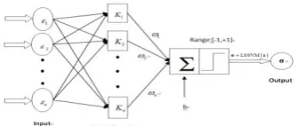
Figure 1. Process flow for a strain-controlled LSSVM model

When strain variables

ε

_{are given as input, and} stress variables

σ

_{are given as output, the general form} of a strain-controlled LSSVM model can be expressed as :

(7)  

= LSSVM

σ ε

Figure 1 demonstrates the process flow for a strain-controlled LSSVM model. In order to mimic the relationship between strains and stresses, we can set strains to input and stresses to output, and LSSVM uses nonlinear mapping based on kernel functions to convert an input space into a high dimension space, then finds a nonlinear relationship between input and outputs in that space. While stress variables

σ

are given as input, and strain variables

ε

are given as output, the general form of a stress-controlled LSSVM model can be described as:

 

= LSSVM

ε σ (8)

The LSSVM model used in Equations (7) and (8) is referred to as a one-point version, because the forms include the current state of variables only. One-point models are suitable for moderately path dependent or independent path behavior. For the sake of representing strongly dependent path material behavior, a two-point version model and a three-point version model can be expressed as:

 



   1



= LSSVM ,

n n n

σ ε ε (9)

 



   1



= LSSVM ,

n n n

ε σ σ (10)

 



    1 2



= LSSVM , ,

n n n n

σ ε ε ε (11)

 



   1  2



= LSSVM , ,

n n n n

ε σ σ σ (12)

where the superscript (n) represents the current state of stress and strain variables, and the superscripts(n-1)and (n-2) represent two previous stresses and strains variables along the loading path. The LSSVM modeling version used in Equations (9) and (10) is described as a two-point version, including the current state and one history point, and the LSSVM modeling version used in Equations (11) and (12) is described as a three-point version, including the current state and two history points.

Meanwhile, with increasing the number of history points in LSSVM modeling, it is able to represent dependent path material behavior better and better. These LSSVM models can be expressed generally as:

 



    1 2



= LSSVM , , ,

n n n n

σ ε ε ε (13)

 



   1  2



= LSSVM , , ,

n n n n

ε σ σ σ ₍₁₄₎

We can realize that, the aforesaid LSSVM models will be more and more complex with increasing the number of history points. As will be seen later in this paper, the three versions of LSSVM models will be used to simulate the constitutive relationship of clay.

4. LSSVM MODELING OF UNDRAINED AND DRAINED BEHAVIOR OF CLAY

LSSVM will be applied in modeling of the undrained and drained behavior of clay in this section. The capability of the three version of LSSVM models in simulating and predicting undrained and drained behavior of clay has been examined under triaxial compression condition on normally consolidated Fujinomori clay [23-25] (experimental data from Nakai and Matsuoka; Nakai et al.), and the modified Cam-clay model has been compared by the three models respectively, because the modified Cam-clay model is acknowledged as the most successful model of clay. The values of Fujinomori clay parameters used in the models are listed in Table 1.

The aim is to use the experimental data to train the three LSSVM models to simulate and predict Fujinomori clay in both undrained and drained tests for initial void ratio 0.68 and confining pressure 196 kPa. A total number of 74 undrained and 68 drained triaxial test samples are used as the database. The undrained or drained test sample points will be divided into two groups randomly，one of the groups is used in training the LSSVM models, the other group (selected 4 samples of each test) is used to test the performance of the trained LSSVM models. In the following narration, there are two subsections for the three LSSVM models on the undrained and drained conditions, respectively.

4. 1. LSSVM Models for Constitutive Relationship On Undrained Tests Firstly, a one-point LSSVM model is developed to express the constitutive relationship, and then the history points will be added to the models. The one-point LSSVM model can be written in the following form:

 



 



0 LSSVM1 ,

n n

e



In this equation, _σ=



_{p q}_,



, ₌



_,



v d

 

ε ,

e

₀ denotes

initial void ratio, mean effective stress





1 2 3 3

p   ,

deviator stress

1 3

q  , volumetric strain

1 2 3 v

    , deviator strain

1 3 d

    , 1

 is axial

stress,

 

₂= ₃ is lateral stress,



₁ is axial strain,

 

₂

=

₃

is lateral strain,

i i u

    , _i_{1, 2,3},

u

denotes pore pressure. It is worth mentioning that, volumetric strain

v



is always zero in the undrained LSSVM models, and void ratio is invariable approximately, so deviator strain

d



and initial void ratio

e

₀ are actually given as input in undrained models. However, volumetric strain and void ratio are variable in the drained LSSVM models, and then the input in drained models should include volumetric strainandvoid ratio along the loading path.

The two-point LSSVM model is obtained by attaching a history point added to the one-point model. The two-point LSSVM model can be written in the following form:

 



   -1



0

LSSVM2 , ,

n n n

e



σ ε σ (16)

Then, the three-point LSSVM model is obtained by attaching two history points added to the one-point model. The three-point LSSVM model can be written in the following form:

 



   -1  -2



0

LSSVM3 , , ,

n n n n

e



σ ε σ σ (17)

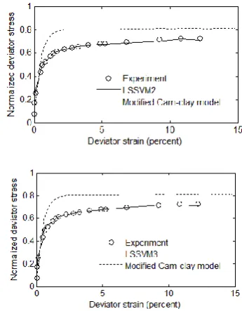
In the following, we can train the above three LSSVM models. Figure 2 shows the performance of the one-point model LSSVM1, the two-point model LSSVM2 and the three-point model LSSVM3 of undrained condition on Fujinomori clay, in terms of the relation between the normalized deviator stress

0

q p (P0=196 kPa) and the deviator strain



_d.

According to Figure 2, the three LSSVM models perform much better than modified Cam-clay model, however, to evaluate further the performance of the three LSSVM models, they should be used to test the other group of sample points.

Figure 2. Performance of LSSVM models on undrained compression tests

A relative error index defined by the following equation can provide a measure of the accuracy of LSSVMs in modeling clay behavior:

0

0 1

1 n

L n

i i

i i

y y Relative Error Index

y 







₍₁₈₎

where n is the number of sample points, L

y denotes the

output of LSSVM models and 0

y denotes the corresponding values of samples. The relative error index can be used to calculate training errors and test errors.

The results in term of relative error indices for all the training and testing cases are summarized in Tables 2. Table 2 is presented separately for each output variable of the three LSSVM models, and the third columns of training and testing case show the combined relative errors. It can be observed that the relative errors of deviator stresses are larger than the values of mean effective stresses, but the combined relative errors should be acceptable, and it is able to demonstrate the good performance of the three LSSVM models once again.

variables in this part. Firstly, the one-point version, two-point version and three-two-point version LSSVM models of expressing stress variables by strain variables (i.e. strain-stress relationship) can be written in the following forms:

 n _LSSVM1



   n_, n



e



σ ε ₍₁₉₎

 



     -1



LSSVM2 , ,

n n n n

e



σ ε σ ₍₂₀₎

 



   -1    -2



LSSVM3 , , ,

n n n n n

e



σ ε σ σ (21)

Compared to Equations (15), (16) and (17), initial void ratio

0

e should be replaced by void ratio of current state  n

e , mean effective stress

p



equals to mean effective p approximately, and volumetric strain



_v is not zero. Secondly, the three LSSVM models of expressing strain variables by stress variables (i.e. stress-strain relationship) can be expressed in the following equations:

 



   



LSSVM1 ,

n n n

e



ε σ (22)

 



     -1



LSSVM2 , ,

n n n n

e



ε σ ε (23)

 



       -1 -2



LSSVM3 , , ,

n n n n n

e



ε σ ε ε (24)

Compared to Equations (19), (20) and (21), except for switching the input variables and output variables, the variables reflecting path are strains in Equations (23) and (24).

Then, we can train the three LSSVM models for strain-stress and stress-strain relationship. Figure 3 shows the strain-stress performance of the one-point LSSVM1, the two-point LSSVM2 and the three-point LSSVM3 of drained condition on Fujinomori clay, in terms of the relation between the principal stress ratio

1 3

  and the axial strain



₁. The principal stress ratio

1 3

  and the axial strain



₁ can be calculated by the following equations:

1

3

3 2

3

p q p q

 

 

 (25)

1

2 3

v d

 

   (26)

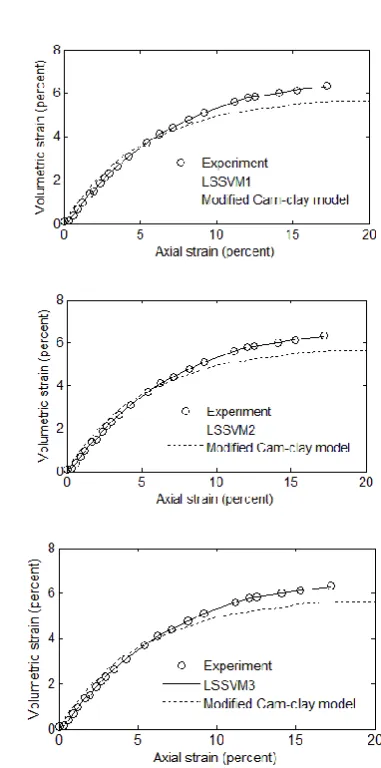
Figure 4 shows the stress-strain performance of the three LSSVM models of drained condition on Fujinomori clay, in terms of the relation between the volumetric strain



_v and the axial strain



₁.

According to Figure 3 and 4, the three LSSVM strain-stress and stress-strain models perform also better than modified Cam-clay model. Furthermore, they

should be used to test the other group of sample points. The relative errors of the two kinds of LSSVM models can be calculated by Equation (18), and the results are listed in Table 3 and 4.

TABLE 2. The relative errors for LSSVM models on undrained compression tests

Training case

Output variable p(%) q(%) Combined(%)

LSSVM1 0.45 9.57 5.01

LSSVM2 0.25 4.38 2.32

LSSVM3 0.30 5.46 2.88

Testing case

Output variable p(%) q(%) Combined(%)

LSSVM1 1.56 9.51 5.54

LSSVM2 2.00 11.77 6.89

LSSVM3 1.67 10.36 6.02

Figure 4. Performance of LSSVM stress-strain models on drained compression tests

TABLE 3. The relative errors for LSSVM strain-stress models on drained compression tests

Training case

Output variable p(%) q(%) _Combined(%)

LSSVM1 0.62 8.22 4.42

LSSVM2 0.47 6.22 3.35

LSSVM3 0.52 6.51 3.52

Testing case

Output variable p(%) q(%) _Combined(%)

LSSVM1 2.03 10.32 6.18

LSSVM2 2.89 12.78 7.84

LSSVM3 3.11 13.82 8.47

TABLE 4. The relative errors for LSSVM stress-strain models on drained compression tests

Training case

Output variable v(%) d(%) Combined(%)

LSSVM1 0.21 0.66 0.44

LSSVM2 0.21 1.01 0.61

LSSVM3 0.18 1.06 0.62

Testing case

Output variable v(%) d(%) Combined(%)

LSSVM1 10.95 20.23 15.59

LSSVM2 9.54 19.20 14.37

LSSVM3 7.84 18.70 13.27

The structure of Tables 3 and 4 is same as Table 2, it can be observed that the relative errors of deviator stresses are also larger than the values of mean effective stresses in Table 3, and testing errors are larger than training errors in Table 3 and 4. But the combined relative errors of strain-stress models are no more than 9%, stress-strain models are not exceeding 16%, however, it is enough for practical engineering problems. On the other hand, the two kinds of LSSVM models perform much better than modified Cam-clay model, so the results of LSSVM models should be acceptable.

5. CONCLUSIONS

Least squares support vector machine (LSSVM) which is a robust type of SVM offers an effective alternative for simulating constitutive modeling of clay. In the present research, three versions of LSSVM models are set up by adding more history points, though LSSVM models will be more and more complex with increasing the number of history points, they represent dependent path material behavior better and better. The good performance of the LSSVM models is demonstrated by simulating and prediction of constitutive relationship of clay under undrained and drained conditions. Comparing with conventional modeling methods, i.e. modified Cam-clay model, LSSVM models need not assumptions and calculation of parameters in a mathematical model, and LSSVM just utilizes experimental data to set up models, thus more objectively and accurately. In contrast to artificial neural networks (ANN) and support vector machine (SVM), LSSVM can overcome some shortcomings of ANN or SVM models, and LSSVM works very well for all the complex situations, thus more effectively.

In the future step, the models of LSSVM can be coupled with finite element methods in numerical analysis. On the other hand, if there are more effective data, LSSVM models can express behavior of clay under some complex stress states with the increase in the number of history points.

6. ACKNOWLEDGMENTS

The research in this paper is funded by China National Science Foundation under Grant No. 11172088. This support is gratefully acknowledged.

7. REFERENCES

on numerical methods in engineering: theory and applications, Swansea, UK., (1990), 701-717.

2. Ghaboussi, J ,.Lade, P. and Sidarta, D., "Neural network based modelling in geomechanics", in Proceedings of the 8th International Conference on Computer Methods and Advances in Geomechanics, Morgantown, WV., (1994), 153-164. 3. Ellis, G., Yao, C., Zhao, R. and Penumadu, D., "Stress-strain

modeling of sands using artificial neural networks", Journal of

Geotechnical Engineering, Vol. 121, No. 5, (1995), 429-435.

4. Penumadu, D. and Zhao, R., "Triaxial compression behavior of sand and gravel using artificial neural networks (ann)",

Computers and Geotechnics, Vol. 24, No. 3, (1999), 207-230.

5. Pernot, S. and Lamarque, C.-H., "Application of neural networks to the modelling of some constitutive laws", Neural Networks, Vol. 12, No. 2, (1999), 371-392.

6. Zhao, H., Huang, Z. and Zou, Z., "Simulating the stress-strain relationship of geomaterials by support vector machine",

Mathematical Problems in Engineering, Vol. 2014, (2014).

7. Ghaboussi, J., Garrett Jr, J. and Wu, X., "Knowledge-based modeling of material behavior with neural networks", Journal

of Engineering Mechanics, Vol. 117, No. 1, (1991), 132-153.

8. Ghaboussi, J., Zhang, M., Wu, X. and Pecknold, D., "Nested adaptive neural network: A new architecture", in Proceeding, International Conference on Artificial Neural Networks in Engineering, (1997), 67-72.

9. Ghaboussi, J. and Sidarta, D., "New nested adaptive neural networks (nann) for constitutive modeling", Computers and

Geotechnics, Vol. 22, No. 1, (1998), 29-52.

10. Sidarta, D. and Ghaboussi, J., "Constitutive modeling of geomaterials from non-uniform material tests", Computers and

Geotechnics, Vol. 22, No. 1, (1998), 53-71.

11. Zhu, J.H., Zaman, M.M. and Anderson, S.A., "Modelling of shearing behaviour of a residual soil with recurrent neural network", International Journal for Numerical and Analytical

Methods in Geomechanics, Vol. 22, No. 8, (1998), 671-687.

12. Zhu, J.-H., Zaman, M.M. and Anderson, S.A., "Modeling of soil behavior with a recurrent neural network ,"Canadian

Geotechnical Journal, Vol. 35, No. 5, (1998), 858-872.

13. Banimahd, M., Yasrobi, S. and Woodward, P., "Artificial neural network for stress–strain behavior of sandy soils: Knowledge based verification", Computers and Geotechnics, Vol. 32, No. 5, (2005), 377-386.

14. Park, D. and Rilett, L.R., "Forecasting freeway link travel times with a multilayer feedforward neural network", Computer‐Aided

Civil and Infrastructure Engineering, Vol. 14, No. 5, (1999),

357-367.

15. Vapnik, V., "The nature of statistical learning theory, Springer Science & Business Media, (2013).

16. Samui, P., "Slope stability analysis: A support vector machine approach", Environmental Geology, Vol. 56, No. 2, (2008), 255-267.

17. Suykens, J.A. and Vandewalle, J., "Least squares support vector machine classifiers", Neural Processing letters, Vol. 9, No. 3, (1999), 293-300.

18. Vapnik, V.N., "An overview of statistical learning theory",

Neural Networks, IEEE Transactions on, Vol. 10, No. 5,

(1999), 988-999.

19. Vapnik ,V., Golowich, S.E. and Smola, A., "Support vector method for function approximation, regression estimation, and signal processing", in Advances in Neural Information Processing Systems 9, (1996).

20. Yarveicy, H., Moghaddam, A.K .and Ghiasi, M.M., "Practical use of statistical learning theory for modeling freezing point depression of electrolyte solutions: Lssvm model", Journal of

Natural Gas Science and Engineering, Vol. 20, (2014),

414-421.

21. Safari, H., Shokrollahi, A ,.Jamialahmadi, M., Ghazanfari, M.H., Bahadori, A. and Zendehboudi, S., "Prediction of the aqueous solubility of baso 4 using pitzer ion interaction model and lssvm algorithm", Fluid Phase Equilibria, Vol. 374, (2014), 48-62. 22. Haji, M.S., Mirbagheri, S., Javid, A., Khezri, M. and Najafpour,

G., "A wavelet support vector machine combination model for daily suspended sediment forecasting", International Journal of

Engineering-Transactions C: Aspects, Vol. 27, No. 6, (2013),

855-864.

23. Matsuor, H ,.Yaoii, Y.-P. and Sun, D., "The cam-clay models revised by the smp criterion", Soils and Foundations, Vol. 39, No. 1, (1999), 81-95.

24. Nakai, T. and Matsuoka, H., "A generalized elastoplastic constitutive model for clay in three-dimensional stresses", Soils

and Foundations, Vol. 26, No. 3, (1986), 81-98.

Least Squares Support Vector Machine for Constitutive Modeling of Clay

X. Zhoua,b_{, J. Shen}c

a _{School of Mathematics and Physics, Huanggang Normal University, Huanggang, Hubei Province, China} b _{School of Mechanics and Materials, Hohai University, Nanjing, Jiangsu Province, China}

c _{School of Civil and Transportation Engineering, Hohai University, Nanjing, Jiangsu Province, China}

P A P E R I N F O

Paper history:

Received 10 July 2015

Received in revised form 27 August 2015 Accepted 16 October 2015

Keywords: Constitutive Modeling Artificial Neural Network Support Vector Machine

Least Squares Support Vector Machine Fujinomori Clay

هديكچ

سر کاخ یراتخاس یزاس لدم هلمج زا

تسا کینکتوئژ یسدنهم رد مهم تاقیقحت .

یارب یضایر قیقد تارابع زا هدافتسا

شنت هطبار نیمخت

سر کاخ شنرک راوشد

ا تس . یعونصم یبصع هکبش

(ANN)

نابیتشپ رادرب نیشام و

(SVM)

اب

دنا هدش هدافتسا سر کاخ یراتخاس یزاس لدم رد تیقفوم .

یبصع هکبش میمعت ییاناوت ،لاح نیا اب اب

زا یخرب

تیدودحم تسوربور اه زا هدافتسا و

SVM

رد م لئاس تسا دودحم یزاس هنیهب لوط رد گرزب سایقم رد عبات بیرقت .

رد

ینابیتشپ رادرب نیشام تاعبرم لقادح ،هلاقم نیا

(LSSVM)

شنت هطبار یزاس هیبش یارب

هدش داهنشیپ سر کاخ شنرک

تسا .

LSSVM

زا یوق عون کی

SVM

تسا هک بوخ یاه یگژیو

SVM

ار ظفح هدرک یایازم یاراد نینچمه و

دوخ درف هب رصحنم .تسا

LSSVM

رثوم نیزگیاج ی

یزاس لدم دیلقت یارب دهد یم هئارا سر کاخ یراتخاس

. درکلمع

لدم بوخ

LSSVM

اس هطبار ینیب شیپ و یریگدای اب یراتخ

سر کاخ

Fujinomori

و هدشن یشکهز طیارش تحت

هداد ناشن کشخ یم

.دوش لدم زا هخسن هس ،رضاح هعلاطم رد

LSSVM

خیرات طاقن نتفرگ رظن رد اب ی

هدش هتخاس رتشیب

تسا . تباث جیاتن یم هک دنک یاه لدم ساسا رب

LSSVM

هدش حلاصا سر کاخ کماداب لدم هب تبسن .دنراد یرترب