*Corresponding author:Manikandan, B ISSN: 0976-3031
Research Article
VECTOR ERROR CORRECTION MODELING FOR INDIAN GDP,
EXPORT AND IMPORT
Manikandan, B* and Rajarathinam, A
Department of Statistics, Manonmaniam Sundaranar University, Abishekapatti, Tirunelveli, Tamil Nadu
DOI: http://dx.doi.org/10.24327/ijrsr.2019.1008.3902
ARTICLE INFO ABSTRACT
The main objective of this paper is to investigate the dynamic relationships between GDP, Export and Import in India using the sixty four yearly data for the period 1950 to 2014. In this paper different econometrics tools viz., Jarque-Bera test (test for normality), Augmented Dickey-Fuller unit root test, Phillips-Perron unit root test and KPSS test (stationarity test - used for the testing stationarity), Johansen Co-integration test (test for the number of con-integrating relationships among the underlying variables) Vector Error Correction Model (to determine long run relationship among the variables) Wald test (test for short run) and Granger Causality test (to detect the direction of causality) have been employed. The stationarity test results indicated that the three variables under study have unit root at level I(0), but after the variables are converted into first difference, they became stationary, I(1). The trace and Max-eigen value test statistics of Johansen’s Co-integration test indicated the existence of two co-integrating equations and exhibited a long-run equilibrium relationship exists between the study variables. In the Vector Error Correction Model, C(1) is the co-efficient of error correction (co-integration) model which is negative and significant indicating that there is a long run causality running from import and export to GDP. The Wald test indicates that there exists short run causalities running from export to GDP and there is no short run causality running from import to GDP. The Granger Causality test reveals that there exists bidirectional causality between export and GDP and unidirectional causality running between import and GDP. The residuals due to Vector Error Correction Model are independently (no autocorrelation) and normally distributed. Also the VECM model is free from Heteroskedasticity.
INTRODUCTION
When a country exports goods, it sells them to a foreign market, that is, to consumers, businesses, or governments in another country. Those exports bring money into the country, which increases the exporting nation's GDP. When a country imports goods, it buys them from foreign producers. The money spent on imports leaves the economy, and that decreases the importing nation's GDP. Exports and imports play an integral role in determining the trade balance of a country. It is known that exports are seen as engine of economic and social development because of their ability to influence economic growth and poverty reduction. If net exports are positive, the nation has a positive balance of trade. If they are negative, the nation has a negative trade balance. Virtually every nation in the world wants its economy to be bigger rather than smaller. That means that no nation wants a negative trade balance. Every nation are concerned about improving the quality of life of their country man, for this increasing the GDP is of prime
importance for any nations economy. To design and evaluation of current and future economic policies, the knowledge of whether exports and imports are co-integrated with GDP is very much importance.
The aim of this work is to investigate the relationship between GDP, exports and imports. In particular, this work tries to empirically investigate whether there is a long run or short run relationship between GDP, exports and imports of India which is very much essential for the design and evaluation of current and future macroeconomic policies.
Rest of the study is organized as follows. Section II includes the literature survey of some past studies in order to know the empirical evidence for the nature of relationship between exports and imports. Sources of data and methodology are described in Section III. Section IV presents the discussion on the estimated results. Final section concludes the study with some policy implications.
International Journal of
Recent Scientific
Research
International Journal of Recent Scientific Research
Vol. 10, Issue, 08(G), pp. 34473-34478, August, 2019
Copyright © Manikandan, B and Rajarathinam, A, 2019, this is an open-access article distributed under the terms of the Creative Commons Attribution License, which permits unrestricted use, distribution and reproduction in any medium, provided the original work is properly cited.
DOI: 10.24327/IJRSR
CODEN: IJRSFP (USA)
Article History: Received 6th May, 2019
Received in revised form 15th June, 2019
Accepted 12th June, 2019
Published online 28th August, 2019
Key Words:
REVIEW OF LITERATURE
Adeleye (2015) confirmed the existence of linear relationship between export and growth in Nigeria. Furrukh (2015) revealed that there is a strong positive long run as well as short run relationship between exports and economic growth in Pakistan. Muhammad (2015) found that there is no empirical evidence in support of export lead growth hypothesis for Sri Lanka. Azeez and Dada (2014) evidenced that international trade has a significant positive impact on economic growth. Imports, Exports and Trade Openness have significant effect on the economy in Nigeria. Deepika (2014) showed that there does not exist long run equilibrium relationship between exports and GDP per capita. Granger causality test exhibits bidirectional causality running from exports to GDP per capita and GDP per capita to exports in India. Seyed (2014) showed that there is evidence of unidirectional causality between export and economic growth for India. In fact, the economic growth causes export growth. Jayachandran (2013) revealed that GDP has a positive and significant impact on India’s real exports in the long-run, but the impact turns out to be non-significant in the short-run. These reviews observed the presence of causality relationship between growth and macroeconomic variables. The theoretical and conceptual frame work motivated to test the individual and joint causal relationship between GDP, export and import using sixty four yearly data for the period 1950 to 2014.
MATERIALS AND METHODS
Materials
The time-series data on Gross Domestic Product (GDP), Indian Import (Im) and Export (Ex) yearly trade prices data from 1950 to 2014 have been collected through the web site https://central statistical organisation.com.
Methods
In this paper different econometrics tools viz., Jarque-Bera test (test for normality),Augmented Dickey-Fuller unit root test, Phillips-Perron unit root test and KPSS test (stationarity test - used for the testing stationarity), Johansen Co-integration test (test for the number of con-integrating relationships among the underlying variables), Vector Error Correction Model (to determine long run relationship among the variables), Wald test (to identify the short run relationship among the variables) and Granger Causality test (to detect the direction of causality) have been employed. These procedure details are discussed as follows.
Unit Root Test
To check the stationary property of all the variables used in the study three different test viz., Augmented Dickey-Fuller unit root test (ADF) (Dicky and Fuller, 1979), the Phillips-Perron unit root test (PP) (Phillips and Perron,1988) and KPSS test (Kwiatkowski, Phillips, Schmidt, Shin,1992) both with trend and trend & intercept have been employed.
Johansen Co-integration Test
Cointegration, an econometric property of time series variables, is a precondition for the existence of a long run or equilibrium econometric relationship between two or more variables having unit roots, integrated of order one. The Johansen approach
shows that two or more random variables are cointegrated if each of the series is themselves non-stationary, and they have a long run equilibrium relationship among the variables. The purpose of the co-integration test is to determine whether a group of non-stationary series is cointegrated or not. The precondition for applying Johansen Cointegration test is the variables must be non-stationary at level but when convert all the variables into first difference then they will become stationary. All the variables should be integrated of same order. The presence and the number of co-integrating relationships among the underlying variables are tested through the Johansen procedure i.e., Johansen and Juselius (1990) and Johansen (1991). Specifically, the maximum eigenvalue test and trace test are used to test for the number of co-integrating vectors. The maximum eigenvalue statistic tests the null-hypothesis of r cointegrating relations against the alternative r+1 conintegrating relations for r=0,1,2,…,n-1. This test statistics are computed as:
)
1
log(
))
1
/(
(
*max
r
n
T
LR
Trace statistics investigate the null-hypothesis of r cointegrating relations against the alternative of n cointegrating relations, where n is the number of variables in the system for r=0,1,2,3,…,n-1. Its equation is computed according to the following formula:
n
r i
tr
r
n
T
LR
1 *
)
1
log(
)
/
(
where λ is the maximum eigenvalue and T is the sample size. In some cases Trace and Maximum Eigen value statistic may yield different results and Alexander (2001) indicates that in this case the results of trace test should be preferred.
Vector Error Correction Model
Vector Autoregressive (VAR) is one of the special forms of system simultaneous equation. Model VAR can be applied if all the variables are stationary. However, if the variables in vector Zt are non-stationary, then the model used is Vector
Error Correction Model (VECM) if there exist at least one or more cointegration relationship exists among the variables. VECM is VAR which has been designed for use whit non-stationary data having cointegration relationship.
VECM is one of the time series modeling’s which can directly estimate the level to which a variable can be brought back to equilibrium condition after a shock on other variables. VECM is very useful by which to estimate the short term effect for both variables and the long run effect of the time series data. The VECM (p) with the cointegration rank r ≤ k is as follows:
t t p
i i t
yt
c
Y
Y
11
1
1
where:
: Operator differencing, where
y
t
y
t
y
t1 yt-1 : Vector variable endogenous with the 1st lag.t
: Matrix coefficient of cointegration
'
;
Vector adjustment, matrix with order (k × r) and
Vector cointegration (long-run parameter) matrix (k × r).i
: Matrix with order k × k of coefficient Endogenous of the ith variable.Wald Test
The short-run causality is also tested using Wald test. The Wald test computes a test statistic based on the unrestricted regression. The Wald statistic measures how close the unrestricted estimates come to satisfy the restrictions under the null-hypothesis. If the restrictions are in fact true, then the unrestricted estimates should come close to satisfy the restrictions.
Testing for causality
Testing causal relations between two stationary series Xt and Yt can be based on the following bivariate autoregression (Granger,1969).
where p is a suitably chosen positive integer;
k’s and
k’s , k=0,1,2,3,…,p are constants; andu
t and
tusual disturbance terms with zero means and finite variances. The null-hypothesis that Xt does not Granger-cause Yt is rejected ifthe
k’s, k>0 in the first equation are jointly significantly different from zero using a standard joint test (e.g., an F test). Similarly, Yt Granger-causes Xt if the
k ’s, k>0 coefficients in the second equation are jointly different from zero. A bi-directional causality (or feedback) relation exits if both
k’s and
k’s, k>0 are jointly different from zero.It may be mentioned that the above test is applicable to stationary series. In reality, however, underlying series may not be non-stationary. In such cases, one has to transformed the original series into stationary series and causality test would be performed based on transformed stationary series.
RESULTS AND DISCUSSION
As per the literature survey, all data series of the study variables have been transformed to natural logarithms. Graph 1, 2 and 3 depict the line graphs of raw data, log data and the first difference of log data, respectively. The time plot for GDP, EXPORT and Import shows a long-run movement of the value of the series in the same direction over the period considered and this indicates a secular movement. The descriptive analysis is used to summarize the characterize of the variables.
Graph 1 Line graph of the GDP (Y), Export (EX) and Import (IMP)
Graph 2 Line graph of the log values of GDP (Y), Export (EX) and Import
(IMP)
Graph 3 Line graph of the first difference values of GDP (Y), Export (EX) and
Import (IMP)
Descriptive Statistics
The descriptive statistics of the study variables are presented in the table 1. The results shows that mean and median values are found to be same for all the three study variables. The skewness is positive which indicate that the upper tail of the distribution is thicker than the lower tail. This implies that the study variables do not decline more often. The kurtosis coefficient values is positive and found to be less than 3, which indicates that the distribution to be platykurtic with fewer and less extreme outliers. Also the Jarque-Bera test statistics suggest that all variables are normally distributed.
0 2000000 4000000 6000000 8000000 10000000 12000000
1 4 7 10 13 16 19 22 25 28 31 34 37 40 43 46 49 52 55 58 61 64
Y EX
P
ri
ce
OBS
0 2 4 6 8 10 12 14 16 18
1 4 7 10 13 16 19 22 25 28 31 43 37 40 43 46 94 52 55 58 61 64
LogY LogEx
P
ri
ce
OBS
-100000 100000 300000 500000 700000 900000 1100000 1300000
1 4 7
10 13 16 19 22 25 28 31 34 37 40 43 46 49 52 55 58 61 64
D(Y) D(Ex)
P
ri
ce
Table 1 Descriptive Statistics
LOGY LOGEX LOGIMP
Mean 12.2528 9.4803 9.7903 Median 12.0396 9.0227 9.5429 Maximum 16.1642 14.4543 14.8140 Minimum 9.2139 6.2747 6.4101
Std. Dev. 2.1837 2.6396 2.6399 Skewness 0.2011 0.3650 0.4006 Kurtosis 1.7254 1.7740 1.8608 Jarque-Bera 4.7632 5.4294 5.1721 Probability 0.0924 0.0662 0.0753
Unit Root Test
The results of the ADF, PP and KPSS tests are reported in table 2. The result shows that the study variables viz., GDP, import and export are non-stationary in levels but the null-hypothesis of non-stationarity is rejected at the 1 % levels of significance after variables have been first differenced. The result indicates that the three variables under study have unit root at level I(0), but after the variables are converted into first difference, they became stationary, I(1).
Table 2 Characteristics of ADF, PP and KPSS Unit Root tests
Augmented Dickey-Fuller
test statistic
Phillips-Perron
test statistic KPSS test statistic
Tr
end
Variable Level First
Difference Level
First
Difference Level
First Difference
ln Y 3.9039 -5.6597** 3.2897 -5.7332** 1.0164 0.7117**
ln EXP 3.5299 -5.9150** 3.0299 -6.2034** 0.9990 0.6808**
ln IMP 2.2797 -6.4859** 2.5095 -6.5504** 1.0012 0.6002**
Tr
end
a
nd
Int
er
cept ln Y -3.8153 -6.8407** -3.8153 -6.8628** 0.2394 0.1714**
ln EXP -3.0357 -7.5481** -3.0357 -7.6162** 0.2365 0.1331**
ln IMP -1.8074 -7.4412** -1.7648 -7.4455** 0.2445 0.0732**
** Significant at 1 % level ; Values in ( ) indicates corresponding p-values
Here all the three variables are integrated of same order. Meaning that at level they are non-stationary but when convert them to first difference, then they become stationary. When the variables are integrated of same order one can run the Johansen Cointegration test.
Johansen’s Co-integration test
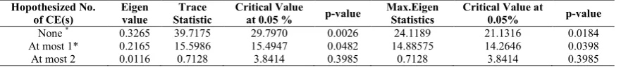
Johansen’s cointegration test is applied to find stationary linear combination and long-run cointegrating equilibrium among the non-stationary variables. The results of both trace statistics and the maximum eigen value test statistics are presented in table 3. The null-hypothesis of no co-integration equation is strongly rejected with a probability of 5 %. Both the trace statistics and maximum eigen statistics rejects the null-hypothesis of at most 1. That is, there is, existence of at most two co-integrating equations among the variables. The results shows that a long-run equilibrium relationship exists between the variables under study. But in the short-run there may be deviations from this equilibrium, and it is required to verify whether such disequilibrium converges on the long-run equilibrium or not. Thus, Vector Error Correction Model is used to generate such short-run dynamics.
Vector Error Correction Model
As the three study variables are co-integrated one can run the Vector Error Correction Model. Here GDP is considered as the dependent variable and the import and export as considered as the independent variable and the characteristics of target model is presented in the table 4 and the VECM model is given by D(LOGY, 2) = C(1) * (D(LOGY(-1)) - 0.5018 * D(LOGEX(-1)) - 0.0468) + C(2) * D(LOGIMP(-D(LOGEX(-1)) - 0.7831 * D(LOGEX(-1)) - 0.0336) + C(3) * D(LOGY(-1),2) + C(4) *D(LOGIMP(-1),2) + C(5) * D(LOGEX(-1),2) + C(6) * D(LOGEX(-2),2) + C(7) * D(LOGIMP(-2),2) + C(8) * D(LOGEX(-2),2) + C(9)
Here C(1) is the co-efficient of error correction (co-integration) model which is negative and significant indicating that there is a long run causality running from import and export to GDP. This further explains that there exists long run influence of both the independent variable Import and Export. The coefficients C(2), …, C(7) are called short run coefficient.
The result further shows that overall goodness of fit of the model shown by the R2 is highly significant which means the independent variables export and imports are able to explain almost 51 % of the changes in the dependent variable GDP. This is because of other variables will be influencing the GDP. The value of D-W statistics is nearly equal to two indicating that the residuals due to this VECM are independently distributed. To ensure consistency of the VECM model, model diagnostics would be carried out.
In order to investigate the short run causality between the export and GDP, Wald statistics have been calculated for the null-hypothesis H0=C(4)=C(5)=0 (H0:No influence in the short
run) and reported in the table 5. As the Chi-square statistics is significant indicating that C(4) and C(5) are not jointly zero and there is short run causality running from export to GDP. Thus with respect to export there are both long run and short run influence on GDP.
In order to investigate the short run causality between the import and GDP, Wald statistics have been calculated for the null-hypothesis H0=C(6)=C(7)=0 (H0:No influence in the short
run) and reported in the table 6. As the Chi-square statistics is non-significant indicating that either C(6) or C(7) is zero and there is no short run causality running from import to GDP. Thus with respect to Import only the long run causality and short run causality running form import to GDP.
Model error diagnostics
Usually when the analysis involves time series data, the possibility of autocorrelation is high. So it is necessary to test the residuals for autocorrelation using the Breusch-Godfrey LM test. The result presented in the table 7 reveals that the null-hypothesis of no serial correlation is accepted since the p-value of the test is greater than 5 % and hence there is no serial correlation.
Table 3 Characteristics of Johansen’s Co-integration test
Hopothesized No. of CE(s)
Eigen value
Trace Statistic
Critical Value
at 0.05 % p-value
Max.Eigen Statistics
Critical Value at
0.05% p-value
None * 0.3265 39.7175 29.7970 0.0026 24.1189 21.1316 0.0184
At most 1* 0.2165 15.5986 15.4947 0.0482 14.88575 14.2646 0.0398
Table 4 Characteristics of fitted VECM model
Variable Coefficient Std. Error t-Statistic Prob.
C(1) -0.4688 0.2164 -2.1660 0.0350
C(2) 0.0841 0.0947 0.8878 0.3788
C(3) -0.3832 0.1757 -2.1811 0.0338
C(4) 0.0071 0.0731 0.0974 0.9228
C(5) -0.0039 0.0987 -0.0391 0.9690 C(6) -0.3622 0.1296 -2.7956 0.0073 C(7) -0.0081 0.0507 -0.1606 0.8730
C(8) 0.0388 0.0677 0.5725 0.5695
C(9) 0.0017 0.0057 0.2973 0.7675
R-squared 51 % Mean dependent variable 0.0004 Adjusted R-squared 44 % S.D. dependent variable 0.0581 S.E. of regression 0.0436 Akaike info criterion -3.2878 Sum squared resid 0.0972 Schwarz criterion -2.9736 Log likelihood 107.6334 Hannan-Quinn criter. -3.1649 F-statistics 6.7001 Durbin-Watson stat 1.7810 Prob(F-statistics) 0.0000
Table 5 Characteristics of Wald test for the variables EXPORT and GDP
Test Statistic Value Degree of
Freedom Probability
F-Statistics 4.438528 (2,51) 0.0167
Chi-square 8.877056 2 0.0118
Table 6 Characteristics of Wald test for the variables IMPORT and GDP
Test Statistic Value Degree of
Freedom Probability
F-Statistics 0.209882 (2,51) 0.8114
Chi-square 0.419764 2 0.8107
Table 7 Characteristics of Breusch-Godfrey Serial Correlation LM test for the residual
Test Statistic Value Degree of Freedom Probability
F-Statistics 2.172312 (2,49) 0.1248
Obs*R-squared 4.886667 2 0.0869
Null hypothesis : No serial correlation
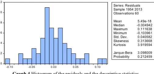
Since the probability of Jarque-Bera test is more than 5 percent, the residual due to the VECM model is normally distributed which is another one desirable quality of the model.
Graph 4 Histogram of the residuals and the descriptive statistics
In order to ensure the consistency, the study further employed Breusch-Pagan-Godfrey heteroskedastic test and the results are presented in the table 8. The result reveals that the null-hypothesis of no heteroscedasticity is accepted since the p-value is more that 5%.
Table 8 Characteristics of Heteroskedasticity test : Breusch-Pagan-Godfrey
Test Statistic Value Degree of Freedom Probability
F-Statistics 1.571739 (12,47) 0.1331
Obs*R-squared 17.18247 12 0.1429
Scaled explained SS 18.12241 12 0.1120 Null hypothesis : No Heteroskesasticity
Testing of Causality
In order to check whether there exist any causal relationships among the variables, and to find the direction of the causality, Granger test of causality has been employed and the results are presented in the following table 9.
The result revealed that the null-hypothesis of no causality between export and GDP running from both directions have been rejected and hence it is clear that there exists bidirectional causality between export and GDP. Here GDP causes Export and vice versa.
The null-hypothesis of no causality running from import and GDP has been accepted and the null-hypothesis of no causality running from GDP and import has been rejected and hence there is a unidirectional causality running between GDP and import. The same type of causal relationships exists for import and export.
Table 9 Characteristics of Granger Causality test between Export, Import and GDP
Null Hypothesis Observation
F-Statistics Probability
LOGEX does not Granger Causes LOGY LOGY does not Granger Cause
LOGEX
62
4.6442 0.0135
11.8016 5.E-05
LOGIMP does not Granger Cause LOGY LOGY does not Granger Cause
LOGIMP
62
2.1073 0.1309
5.7739 0.0052
LOGIMP does not Granger Cause LOGEX LOGEX does not Granger Cause
LOGIMP
62
0.0504 0.9509
3.9854 0.0240
CONCLUSIONS
The study reveals that the variables under the study have unit root at level I(0), but after the variables are converted into first difference, they became stationary, I(1). The trace and Max-eigen value test statistics of Johansen’s Co-integration test indicated the existence of two co-integrating equations and exhibited a long-run equilibrium relationship exists between the study variables. In the Vector Error Correction Model, the co-efficient of error correction (co-integration) is found to be negative and significant indicating a long run causality running from import and export to GDP. The Wald test indicates the existence of short run causalities running from export to GDP and there is no short run causality running from import to GDP. The Granger Causality test reveals the existence of bidirectional causality between export and GDP and unidirectional causality running between import and GDP. Acknowledgment
The Corresponding author thanks the University Grants Commission, New Delhi for awarding fellowship under the
0 2 4 6 8 10 12
-0.10 -0.05 0.00 0.05 0.10
Series: Residuals Sample 1954 2013 Observations 60
Mean 5.49e-18
Median -0.004942
Maximum 0.111638
Minimum -0.103961
Std. Dev. 0.040582
Skewness 0.313668
Kurtosis 3.919594
Jarque-Bera 3.098009
scheme of UGC – Basic Scientific Research fellowship to carry out this work.
References
Adeleye J. Adeteye O. & Adewuyi M, (2015). Impact of International Trade on Economic Growth in Nigeria (1988-2012), International Journal of Financial Research, 6(3): 163-172.
Alexander,C. Market models: A guide to financial data analysis. John Wiley & Sons: (2001).
Azeez, B. A. and Dada, S, (2014).Effect of International Trade on Nigreian Economic Growth: The 21st century Experience, International Journal of Economics, Commerce and Management, 2(10): 1-8.
Deepika Kumari, (2014). Export-Led Growth in India: co-integration and Causality Analysis, Journal of Economics and Development Studies, 2(2): 297-310. Dickey, D, and Fuller,W, (1979). Distribution of the
estimators for autoregressive time series with a unit root. Journal of the American Statistical Association, 74 (366): 427-431.
Enders W. Applied econometric time series, New York: John Wiley and Sons: 1 -63, (2015).
Furrukh Bashir (2015). Exports - led Growth Hypothesis: The Econometric Evidence From Pakistan, Canadian Social Science, 11(7): 86-95.
Jayachandran, G. (2013). Impact of Exchange Rate on Trade and GDP for India A Study of Last Four Decade, International Journal of Marketing, Financial Services & Management Research, 2(9): 154-170.
Johansen, S. (1991). Estimation and Hypothesis Testing of Conintegration Vectors in Gaussian Vector Autoregressive Models. Econometrica, 59(6): 1551-1580.
Johansen,S. and Juselius,K.(1990).Maimum likelihood estimation and inference on cointegartion with application to the demand for money. Oxford Bulletin of Economics and Statistics, 52(2): 169-210.
Kirchgassner G, Wolters J. Introduction to modern time series analysis. Berlin: Springer-Verlag: 1 -277, (2007). Kwiatkowski, D., Phillips , P. C. B., Schmidt, P. and Shin, Y.(1992). Testing the Null Hypothesis of stationarity against the Alternative of a Unit Root. Journal of Econometrics, 54:159-179.
Muhammad Tahir (2015). An Analysis of Export Led Growth Hypothesis: Co-integration and Causality Evidence from Sri Lanka, Advances in Economics and Business, 3(2): 62-69.
Phillips, P.C. and Perron, P. (1988).Testing for a unit root in time series regression. Biometrika, 75(2): 335-346. Seyed Mohammadreza Hosseini (2014). An Empirical Study
of Export and Economic Growth in India since 1960: A Co integration Analysis, Iran. Econ. Rev., 18(1): 53-64
How to cite this article:
Manikandan, B and Rajarathinam, A.2019, Vector Error Correction Modeling For Indian GDP, Export and Import. Int J Recent Sci Res. 10(08), pp. 34473-34478. DOI: http://dx.doi.org/10.24327/ijrsr.2019.1008.3902