Adaptive Unstructured Grid Generation Scheme for Solution of the Heat Equation

(1)

ADAPTIVEUNSTRUCTURED GRID GENERATION SCHEME

FOR SOLUTION OF THE HEAT EQUATION

K. Mazaheri, A. Banai and S. A. Seyed-Reyhani

Department of Mechanical Engineering,Sharif Univ. of Tech. Tehran, Iran, [email protected]

(Recived: April 14, 1997 - Accepted in Final Form: June 1, 2000)

An adaptive unstructured grid generation scheme is introduced to use finite volume Abstract

(FV) and finite element (FE ) formulation to solve the heat equ ation with singu lar bou ndary con dit ions. R egu lar gr ids cou ld not ach e ive a ccu r a t e solu t io n t o t his pr oble m . T he gr id generation scheme uses an optimal time complexity frontal method for the automatic generation and delau nay triangu lation of the grid points. The algorithm is incremental, so it is the most appropriate for an adaptive solver. Using adaptive grids, the solution is refined to get enough accuracy in all grid points. Two schemes are applied for the solution of the equations to show the flexibility of the adaptive grid scheme. First a cell-vertex finite volume formulation is used. Then, for the FE scheme, u sing linear shape fu nctions, a set of linear equ ations are solved explicitly, with overrelaxation. A sequence of adaptation is applied and appropriate number of gr id p oin ts a re intr odu ced in finite pred eter min ed form ats to the existen t e leme nts, till convergence in the solution is observed. A postprocess is used to smooth the distribution of the se t of no des. T his p rocedu re is a pplied to a few st u dy ca ses t o sho w tha t the me tho d is convergent, and produces accurate solution even in the case of singular boundary conditions.

Delaunay Grid, Unstructured, Heat Equation Key Words

j°kdÇ« ºAq]A ° j°kd« ©\e ºB´{°n pA ²jB TwA ºAoM » ¼L U ¬B«pBw »M ³ñL{ k¼§±U x°n ð½

²k¼ña

kÇ¯A±U»ªÇ¯ ºA³§BÇv« ¼®Ça nj »§±ªí« ³ñL{ /SwA ²k{ » oí« jkíT« ºpo« ½Ao{ BM RnAoe ³§jBí« ¥e ºAoM ºAoM An k{BM»« ³®¼´M Ao]A ¬B«p o ¯ pA ³ ²k¯°n y¼Q ³´L] x°n ð½ ³ñL{ k¼§±U x°n /k½Bª¯ jB\½A ¼ j JA±] ºjkÇî ¥e ºAoM ° ²j±M »z½Aq A ²k{ ²jB TwA ©T½n±¢§A /jo¼£»« nBñM B´¯C »¯¿j ºk®MW¦X« ° B ¯ nB j±i k¼§±U J±¦ « S j ³M ¬k¼wn BU » B nk ³M An ³ñL{ ¬A±U»« » ¼L U ³ñL{ pA ²jB TwA BM /k{BM»« KwB®« nB¼vM » ¼L U ¦Th« ºjkî x°n °j » ¼L U ³ñL{ ©T½n±¢§A ºo½mQ B í¯A ¬jAj ¬Bz¯ ºAoM /j±ª¯ q½n ,o ¯ jn±« ³ ¯ oµ nj ¥ñ{ éMA±U pA ²jB TwA BM kíM ° ²k{ ²jB TwA »§±¦w tEn j°kd« ©\e ³ MAn ð½ AkTMA /SwA ²k{ ²jB TwA ¥e ºAoM k½k] B ¯ » B nAk « ³M ° ³T n nBñM »§A±T« ¼L U ³¦v¦w ð½ /SwA ²k{ ³T o£ nBñM j°kd« ºAq]A x°n ,» i ½A /jpBw»« nA±ªµ An B ¯ é½p±U xpAjoQ uQ x°n ð½ /SwA ²k{ » oí« ²k{ ¼¼íU y¼Q ºB´¦ñ{ L ³ñL{ ¬Bz¯ An jo ®« ºpo« o{ S§Be nj ¬C S j Hæ±~i ° x°n »½Ao¢ªµ BU ³T n nBñM ³¯±ª¯ ³§Bv« k®a ºAoM k®½Co /kµj

INTRODUCTION

Adaptive solution of t he Laplace equation in two dimensions has several applications in heat transfer and many other disciplines. It will allow to have fe wer numbe r of grid ce lls, and st ill keep a maximum acceptable relative truncation error in the whole computational field. Both the unstructured grid and the adaptation procedure have unique fe ature s to allow a flexible and r o bu st de sir a ble n o de dist r ibu t ion . M a n y

(2)

Methods used for numerical solution of Heat e qu a t io n a r e ve r y dive r se ( se e [6, 7, 8]. However, these methods are only efficient when gradients in the te mpe rature field are finit e. Here we introduce a method which is capable of numerical solut ion of the he at equation in a domain including regions of infinite gradients of temperature.

In this paper, using a frontal approach, an unst ruct ure d grid is ge ne rat e d in the whole fie ld. This grid generation scheme , re quire s minimum input from the user, and works in opt imal time limit s. The n finite volume and element formulations are used to discretize the differential equation within the framework of an unstructured grid. Finally, the adaptation allows to have accurate solutions in problems with high solution gradients.

F inite volume me thods have be e n widely used in compressible flow computations. Their ma in fe a t u r e is t h a t t h e y co n se r ve ma ss, momentum and energy, so they provide a robust sche me to capture flow discontinuitie s [9]. Although discontinuities could not propagate in ellipt ic fields, the unstructured adaptive grid use d here makes it ideal for calculations with discontinuities in the boundary conditions. Here we first review the properties of the D elaunay triangles used in the grid generation procedure. Then, t he frontal approach used here will be e xp la in e d, a n d fin a lly, t h e fin it e vo lu me formulation and t he adapt at ion me thods are presented.

GRID GENERATION PROCEDURE

The space discretizat ion could be

Properties

done in many differe nt ways. If e w se le ct all elements to be triangles, different criteria could be used to establish this discretization. The most fa m o u s me t h o d , wh ich h a s sh o wn ma n y t he o r e t ica l a n d a pp lica t io n p ro p e rt ie s, is D elaunay triangulation Therefore, it is used in

most u nst ru ct u r e d me sh co mp u t a t io n s. I t connects e ach three most closest nodes, in a clo u d o f p o int s, t o e a ch o t h e r . T h e o n ly deficiency of D elaunay triangulation, which is commo n t omo st o t h e r me t h o ds, is t h a t it requires a point s cloud t o be give n. In many applicat ions, ge ne rat ion of such a cloud of points is not so easy. In this paper, ew will use different ways, including a frontal approach [11] to produce the initial grid and to adapt it to the solution. The Delaunay triangulation is the dual of theDirichlet tesselation of t he set of given points. The D irichlet t e sse lat ion is made by det ermining t he Voroni regionswhich are the locus of the closest points of the space, to each point of t he colud In t wo space dime nsions, these regions are polygons, mostly with five to seven sides. If we connect each two nodes with n e igh bo r V o r o n i r e gio n s, we will h a ve a Delaunaytriangulation. Delaunaytriangulation has many different properties [12, 13, 14, 15], which show that it is optimum or suitable for many diffe re nt applicat ions. some o f t he se properties are:

É Uniqueness: The Delaunay triangulation

exists and is unique (except for degenerate cases).

É Out-Circle condition: The circumcircle of a

D elaunay triangle respective to three nodes of a give n set , does not include any ot he r grid point (except for degenerate cases).

É Max-Min property: Delaunay triangulation

ma ximize s t h e min imu m a n gle o f t h e triangulation. This prope rty optimizes the grid for many finite element calculations.

É Nearest Neighbor: The closest grid point to

grid, is conne cted to it. This, in fact, shows the solut ion of the famous Nearest point problem.

É Minimal Roughness: For an arbitrary given

(3)

inte rpolation function f, the roughne ss of this surface (its slope in a sense) is minimal if the triangulation is Delaunay.

Numeri cal Properti es to Us e Frontal

Approach in Delaunay Triangulation

The above mentione d prope rtie s make it simple , p o we r fu l, a n d o p t imu m t o u se D e la u n a y triangulation in many diffe rent applications. G iven the set of grid points, there are se veral differe nt me thods to (D e launay) triangulate them. Bowyer [3] int roduced an incre me nt al (recursive) algorithm which works optimally in t ime comp le xit y ( i.e . O ( n log n ) ). I t u se s Vor onoi re gions for its dat a st ruct ure and t rian gula t ion p ro ce du re . It st a rt s wit h a n (arbitrary) set of phantom nodes, including the convex hull of t he grid point s se t. The n each ne w point is adde d, and necessary changes in the cells with a circumcircle including the new grid p o int ar e ma de . Aft e r fin din g a ne w D elaunay triangulat ion, another grid point is added.The algorithm used here is close to those of Lawson [4] and Watso [5]. this uses Delaunay triangles for its data base. It has a preliminary proce dure to ge nerate an init ial grid, using a fro nt al approach , and t he n uses an ite rat ive procedure to adapt the mesh to the solution.

The procedure for generating the initial grid follows:

É Read the data corresponding to the boundary

points.

É Make a convex hull using four phantom

nodes, including all boundary point s, and (Delaunay) triangulate it.

É Add one by one, new boundary points, and

re triangula t e t h e fie ld. E ach t ria ngle is co nside re d t o be a ba d t r ia ngle , e xce pt otherwise marked.

É The common side between bad and good

triangles constructs the front . Introduce a ne w can did node corr e sponding t o e ach

small side of a bad triangle, which is located o n t he fr on t , a nd e valu a t e t h e spa cin g function at that point.

ÉDelete all candid nodes which are too close to

permanent nodes.

ÉMerge all candid nodes which are too close to

each other.

É Mark the candid nodes as permanent, and

add them one by one to the set of nodes, and retriangulate the field.

É Find the new front, and redo the above

procedure, untill there is no front i.e. no bad triangle.

É After construction of the final mesh, use a

Laplace filt e r to smooth t he grid po ints distribution. This involves moving each grid p o in t t h e a r e a a t t h e ce n t e r o f t h e neighboring cells.

D ata struct ure may strongly

Data Structure

affect the overall efficiency of the algorithm. In this work, our records were triangle based, and e ach re co rd include d the t r iangle numbe r, number of its vertices, its neighbors, and a flag to show if it is a bad or a good triangle. We also used a few small lists and stacks to reduce the time complexity.

This proce dure is used both

Retriangulation

in the frontal me tho d and in t h e adaptatio n procedure. Whenever a new node is introduced t o t h e me sh , a lo cal p r o ce ss re t r ian gu la t e around that new node t o make sure t hat all triangles prese rve D elaunay prope rties. The retriangulation procedure follows:

É Use a search algorithm to find to which old

triangle the new node belongs. Walk search is almost t he simplest way and shows to be efficient. Other tree search methods are also equallyacceptable. Exhaustive search would not be efficient.

É Mark sides of this triangle as the temporary

(4)

node (we call it TEDI).

É Recursively, check to see if any node

ne ighbor t o TE D I satisfie s t he in-cir cle condition for the new node and the vertices of the common edge between new node and t h e n e igh bo r n o de . I f so , t h a t e dge is re move d from TE D I, and t he ne ighbor node and the two corresponding edges are added to the TEDI.

É When TEDI does not change any more,

delete all triangles previously inside TE D I, and connect the new node to all vertices of TEDI.

E a c h n e w t r i a n gl e i s

Goodness Criteria

marked bad, except if the ratio of its smallest to its largest edge is greater than a threshold value

b. In this report b ¿ 0.7. If a triangle is marked bad, and in the first trial (firts addition of a new poin t inside it ) , it is n ot de le t e d, it will be accepted as it is, and will be marked ¨¨good¨¨.

U sing spacing functions is

Spacing Function

standard in grid generation schemes. We define the value of the spacing function for boundary p o in t s a s t h e a ve r a ge d ist a n ce fr o m t h e neighboring nodes. In each triangle, we assume a linear interpolation of the value of the spacing function on the vertices to find its values inside that triangle. Therefore, whenever a new node is introduced, the value of the spacing function at that point could be easily calculated. If h0is

the value of the spacing function at a vertex of a t riangle , and si are outward normals to the

edges, the value of the spacing function at the new node ¨¨a¨¨ is equal to

3

(1) ha = h0 + __-1 õ hisi

2s i=1

To add a new node on each small edge of a bad triangle, we assume that the node produces a new good-looking e quilat eral triangle . O ne ca n sh o w t h a t t h is p ro p o se s t h e dist an ce between the new node and the previous nodes

equal t o hÅ/ [1-(¡3/4)(êh.n)] where, h is the spacing function, hÅ is the average value of the spacing funct ion in nodes on t he small e dge, and n is the normal t o t he me ntione d small edge. This equation may predict bad values for the spacing function in regions of high gradient. T o e n su r e a cce p t a ble va lu e s, we imp o se r e s t r i c t i o n b< 1 / hÅ< 1 /b wh e r e b i s experimentally determined to be about 0.5.

FINITE ELEMENT FORMULATION

To solve the linear equation ê2T=0 on a given D irichlete or Neumann boundary conditions, it is e n o u gh t o fin d T wh ich min imize s t h e functional

(2)

t(T) = ßT.ê2TdW

where Wis the whole domain, which is a surface in two dimensional problems. this functional will allow us to be le ss sensitive in our solution to differentiability of the function T. In this way, it will be easier to work with singular solutions. One can show that with Dirichlete or Neumann boundary condition, this functional has the form

(3)

t(T) = ß||êT||2dW

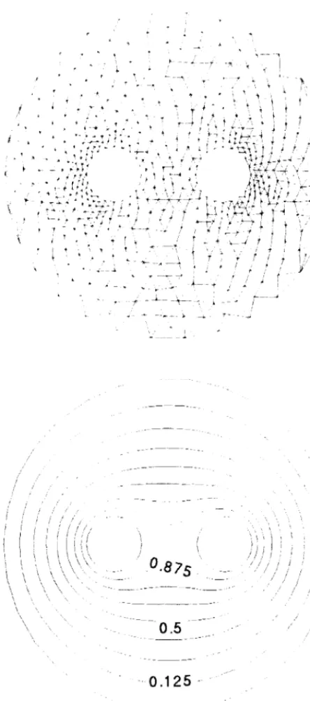
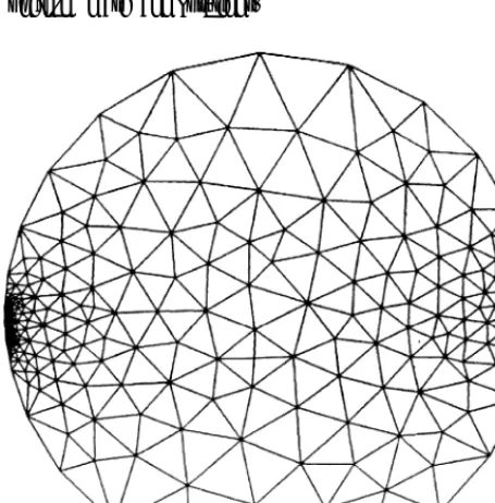
U sing the procedure explained in section 2, we discretize the whole domain to N triangular cells. This triangulation for a circular domain with two cavities is shown in Figure 1. We use a cell-vertex method, i.e. we assume the value of T on all cell vertices (except probably those on t he boundary) t o be unknown. Le t' s assume linear distribution for function T on each cell, i.e. T on cell i is defined as

(4) Ti(x,y)=ai + bix + ciy

which satisfies values of Tj on all vertice s of

triangle i. Finally, the value of T on the whole domain is found to be

N

(5) T(x,y) = õTi(x,y)

i=1

(5)

(a)

(b)

Figure 1.Solution of the Laplace equation on an circular region with two holes a) G rid made by frontal approach after adaptation with e=0.2. b) Solution contours.

One can see that the following matrix

-1

£ Þ £ Þ £ Þ

ai 1 x1 y1 Ti1

(6) bi = 1 x2 y2 Ti2

ci 1 x3 y3 Ti3

¥ ø ¥ ø ¥ ø

gives the coefficient values for each cell i. Here, indices 1, 2 and 3 are corresponding to three ve rt ice s of t r ian gle i. O n e can sh o w t h a t minimization of the functional int roduce d in Equation 1 reduces to the equation

where A.T=B

(7) B=-[Cfp][Tp]

T=[Tf]

A=[Cff]

H e r e , Tf is t h e ve ct o r o f in n e r ve r t ice s

t empe rat ure , and Tp the ve ct or of boundary

vertices temperature. Matrix C is determined so that:

£ Þ £ Þ

Cff Cfp Tf

(8)

t=[TfTp]

Cpf Cpp Tp

¥ ø ¥ ø

a n d co m p o n e n t s o f m a t r ix C co u ld b e geometrically determined, and is a function of the shape functions [16, 17]. To find elements of matrices Cff or Cfpfor each vertex, we should

find contribution of all ce lls sharing in that vertex. Matrix C is symmetric and sparse. Also, summation of e ach row and column of this matrix is equal to zero.

Solution of Equation 2 will give the value of T at each vertex. One way is to find the inverse of the sparse matrix A. Another method, which is mor e po pu la r, is t he family of it e ra t ive methods. Here, we start with an arbitrary initial condition. To have an accurate initial guess, we use a scheme similar to the algorithm used for finding the value s of the space funct ion. The iterative procedure recalculates the value of the temperature at each vertex by

n

(9) Tj = ___-1 õ TiCji

Cjj i=1,iÚj

Since for all nodes not connected to node j the value of cjiis zero, only a few multiplications are

(6)

i

j

DSi,j

(a)

V1

N3

N2

i

V2

V3

j

DSj

N1 Dnj,i

(b)

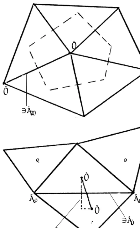
Figure 2.St en cil o f com p u t a t io n in (a ) a ce ll-ve r te x method, (b) a cell-center method.

mat rix wit h space co mp le xit y of O ( N) , and iterate Equation 3 till convergence is acheived ( i.e . norm of T alteration is small e nough). Since C is a positive definite matrix, this method is always convergent [18]. This procedure is in fact an averaging procedure for the temperature of each vertex.

Overrelaxation is also used to increase the convergence rate. We use

n

(10) Tjk+1=(1-w)T jK- __w õ Ticji

cji i=1,iÚj

using values of 1<w<2, rate of convergence will improve.

FINITE VOLUME FORMULATION

To solve t he conse rvation e qu ations on an unstructured grid by finite volume, we may use cell-vertex or cell-center methods. In the first met hod, ew construct our control volumes by connecting t he Voronoi ve rtices around each node (Figure 2a). Inte gration of the Laplace equation on this element results in

n

(11)

õ_____ DSv= 0

Ti-Tj DSi,j j=1

H ere , i is the node in the center of volume element, and j denotes different vertices of this element. T is the temperature, DSi,j is the

distance between nodes and j,DSv is the length

of the corresponding Voronoi polygon edge and n is the number of the edges of the polygon.

In cell-center methods, the unknown is the t e mp e r a t u r e a t ce n t e r o f o u r t r ia n gu la r e le me nt s. I n a first or de r e st ima t ion , on e assume s t hat t he te mpe rature is const ant in each cell, and D elaunay triangles construct our volume elements (Figure 2b). Integration of the Laplace equation over these elements results in:

3

(12)

õ_____ DSj= 0

Ti-Tj Dnj,i j=1

whereDnj,iis the distance of centroids of two

ne ighboring ce lls wit h ce nte rs i and j in t he direction normal to the common edge, DSjis the

length of that edge.

I n t h is wo r k we h a ve u se d t h e fir st formulat ion. Application of t his e quation on each cell produces a linear equation. Writ ing the equations corresponding to all triangular cells will result in a linear system of equations which could be solved with standard methods.

ADAPTATION

(7)

12 7

3 1

Figure 3.Formats used for node addiction.

inverse of t he gradient of the solution at each ce ll. T o do so , using a fro nta l me t hod, we produce an init ial grid and solve t he Laplace e quation ove r it to find an initial nume rical solution. Since most ce lls are coarse at t his st age , this solution is not accurate enough in points with high gradients.

To find cells with highest relative truncation e rror, we nee d a criterion for which we use

dimensionless parameter T*= _______. Here, S¡s|êT| T0

is the area of the corresponding cell, and T0is

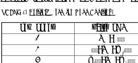
a typical (maximum) value of the temperature on the boundaries. Regions with high values of T* s h o u l d b e r e f i n e d . W e h a ve fo u r p re de t e rmine d for mat s for n o de a ddit io n (Figure 3). According to the value of T*, one of these formats is selected. H ere we use k₁= 1.5, K2=s, k3=3, and these values correspond to cell

sizes in different levels, e determines how small t r u n ca t io n e r r o r we wish . I n r e gio n s o f indefinite solution gradients (singular points) we restrict adaptation levels, or the smallest cell sizes to a predetermined value.

After addition of these new grid points, the re triangulation procedure is re pe ate d, and a

TABLE 1. Criteria Used for Node Addition.

value of T

*

new nodes

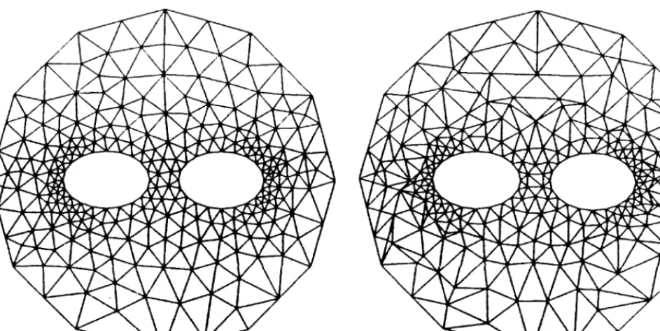
Figure 4.Solution of the Laplace equation on the same region as Figure 1 (a) adapted grid with e=0.1 and (b) grid after filtering postprocess.

cell sizes vary smoothly and rapidly, so some of them are as large as the internal holes.

F igur e 4a is a circula r domain wit h t wo elliptical holes, which is first triangulated with the above mentioned method, but then we have used a Laplace filter to make the grid as smooth as possible. F igure 4b shows the effect of t he filtering.

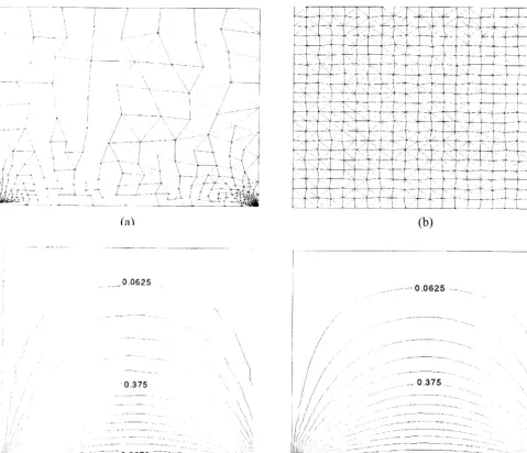
Next, we have solved the Laplace equation on a squa re re gion wit h diffe re nt constant temperatures on lower and the other three sides of the outer boundary by our FEM solver. The length of e ach side of t he square is six. This example is solved t o show both accuracy and effectiveness of the algorithm. Typical solution contours are shown in F igure 5(d). The exact solution of this problem is

sin [___ (x+a/2)]. sinh[___ (a/2-y)]n_ap n_ap T(x,y)= __4 õ_________________________________

p_{odd n} _{n sinh n}_p

(13) First, to show the solution and the effect of the adaptat ion, we have solve d the Laplace equation on that square region on two different

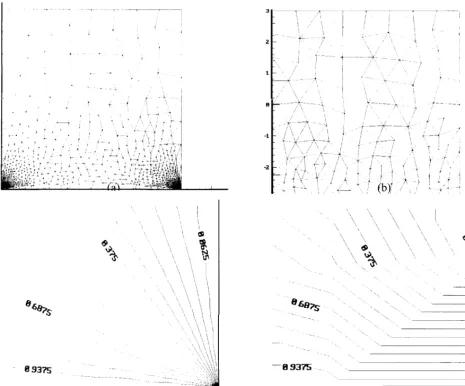
meshes. The first mesh is an almost uniform grid with 270 ce lls. The solut ion is quite accurate everywhere except the small region close to the lower corners (singular points). The solut ion contours only near these corners are shown in F igure ( 6d). To re so lve a be t t e r so lu t ion in these regions. We use the adaptation procedure for seve ral times to get the grid of 2500 cells shown in Figure (6a). The solution contours are now much more accurat e e ven in the re gions colse to the singular point (Figure ( 6c)). This has be e n ve rifie d using the e xact solut ion, Equation 8.

(9)

(a)

(c)

(b)

(d)

Figure 5.Comparison of solutions on uniform and adapted meshes: (a) adapted grid, (b) uniform grid, (c) solution on the adapted mesh and (d) solution contours on the uniform mesh.

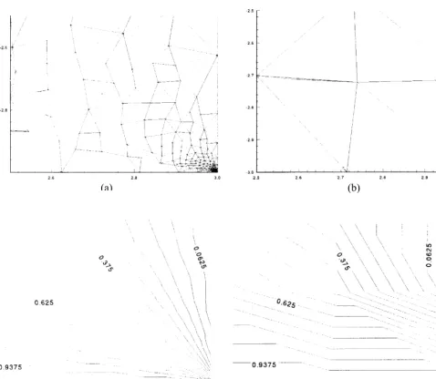
7). This region is almost one hundredth of the total computational fie ld. In this region, t he adapt ed mesh produce s a result very colse to the exact solution (Equation 8), but the uniform grid fails to resolve in an acceptable manner.

Finally to assure the accuracy of the solution, using L2 norm of error (difference of numerical

and exact solutions)is computed, and is drawn versus cell sizes for a uniform mesh (Figure 8). This figure shows that the solution has a second orde r accuracy ( Note t h at t he slope of the

(10)

(a)

(c)

(b)

(d)

Figure 6.Solution of Laplace equation on a square with constant zero temperature on upper and side boundaries and temperature equal to one on lower side: (a) adapted grid, (b) initial grid, (c) solution on the lower corner

in the adapted case and (d) solution contours on the lower corner in the initial mesh.

are continuous, this solution is found to be satisfactory. Many sweeps of adaptation were applied to that solution, and the final grid and solution did not differ in this simple case.

Case two for FVM, is a circular domain, but with temperature equal to 1 on the upper part of the boundary, and equal to zero on the lower part. The grid is se veral times adapte d t o t he new solution and afterwards it is postprocessed (Figure 9). O ne can see that how effective the adaptat ion procedure is in t his more difficult

case. The solut ion contours are not re port ed here.

CONCLUSIONS

(11)

(a)

(c)

(b)

(d)

Figure 7.Comparison of solutions on uniform and adapted meshes: (a) lower corner of adapted grid, (b) lower corner of uniform grid, (c) solution on the lower corner in the adapted case,

and (d) solution contours on the lower corner in the uniform mesh.

t o D elau n ay t riangulat e the m. Appro p riat e merge, delete, and postprocessing procedures were applied to improve the grid quality. After using standard finite element or volume solution of t he pr oble m, a crit e r ion is use d t o find regions with high re lat ive t runcation errors. T h e s e r e gio n s a r e r e f in e d , a n d a f t e r re triangulat ion, and using filte ring proce ss, co mp u t a t io n is r e p e a t e d. T h e D ir ich le t e boundary conditions are applied by determining

(12)

Figure 8. L₂ n o rm of er r o r ve r su s ce ll sizes fo r t h e uniform mesh computations.

Figure 9 . G r id o n a cir cu la r d o m a in wit h sin gu la r boundary condition

_/

REFERENCES

L o , S ., "V o lu m e d isc r e t iza t io n in t o t e t r a h e d r a - I ", 1.

Computers and Structures , Vol. 39, (1991), 493-500. Tipper, J., "Fortran Programs to Construct the Planar 2.

Voronoi Diagram",Computers and Geosciences, Vol. 17, (1991), 597-632.

Bowyer , A., "Com pu t ing D ir ichle t T esse la tion", Th e

3.

Computer Journal , Vol. 24, No. 2, (1981), 162-166. Lawson, C., "Software for C 1 Surface Interpolation", in 4.

Mathematical Software III(J. R ice, ed.), Academic Press, (1997).

Wa tson, D ., "Compu ting t he n-D imensional D e launay 5.

Tesselation with Applications to Voronoi Polytopes",

The Computer Journal, V o l., 24, N o .l2, ( 1981) , 167-172.

R a u sch , R . Ba t in a , J . a n d Y a n g, H ., "Sp a t ia l 6.

Ad apt atio n of U nstru ctu red Me she s for U nstea dy Aerodynamic Flow Computations", AIAAJournal, Vol. 30, (1992), 1243-1250.

St ru ijs, R . V an keirsblick, and D econ inck, H ., "An 7.

Adaptive G rid Polygonal Finite Volu me Method for the Compressible Flow Equations",AIAA-89-1959-CP, (1989).

M a vr ip lis , D . a n d J a m e s o n , A . , "M u lt igr id S o lu t io n o f 8.

t h e T wo D im e n s io n a l E u le r E q u a t io n s o n U n str u ct u re d T riangu la r Meshes",AIAA-87-0353, (1987).

J a m e so n , A ., "T h e E vo lu t io n o f Co m p u t a t io n a l 9.

M e t h o d s in Ae r o d yn a m ics", Journal of Applied Mechanics, Vol. 50, (1983), 1052-70.

B a r t h , T . J . , "A n a lysis o f I m p licit L o ca l L in e a r iz a t io n 10.

Te ch niqu es for U pwind an d TVD Algo rith ms", in

AIAA Paper 87-0595, (January 1987).

M u lle r , J . R oe , P . L. and D econink, H ., "A F r ont al 11.

Approach for Internal Node G eneration in D elau nay Triangulations",International Journal for Numerical Methods in Fluids, (1993).

P r e p a r a t a , F . a n d Sh a m o s, M ., "Co m p u t a t io n a l 12.

Geometry", Springer-Verlag, (1985).

Ba rth , "O n U n st ru ctu r ed G rid s an d So lvers", VK I

13.

Lecture Series 1990-03, (1990).

Baker, T., "Element Quality in Tetrahedral Meshes", in 14.

7th International Conference on Finite Element Methods in Flow Problems, (1989).

R ip p a , S., "M in im a l R o u gh n e ss P r o p e r t y o f t h e 15.

D e la u n a y T r ia n gu la t io n ", P h D T h e sis, T e l-Aviv University, (1989).

S a d i k u , M . , "N u m e r i c a l T e c h n i q u e s i n 16.

Electromagnetics", CRC Press, (1992).

H u ghes, T ., "T he F init e E lem ent M ethod", P r e nt ice 17.

Hall, (1987).

Press, W. Flannery, B. Teu kolsky, S. and Vetterling, 18.