A cure modelling study of an unsaturated polyester resin system for the simulation of curing of fibre-reinforced composites during the vacuum infusion process

A Cure Modelling Study of an Unsaturated Polyester Resin System for

the Simulation of Curing of Fibre-Reinforced Composites during the

Vacuum Infusion Process

Aktas A1_{, Krishnan L}2_{, Kandola B}2_{, Boyd SW}1_{, Shenoi RA}1

1_{Faculty of Engineering and the Environment, University of Southampton, Southampton, SO17 1BJ,} UK

2_{Institute for Materials Research and Innovation, University of Bolton, Bolton, BL3 5AB, UK}

Abstract

This study presents the cure kinetics and the cure modelling of an ambient curing unsaturated polyester (UP) resin system for the simulation of its curing in the vacuum infusion (VI) process. The curing of the thermoset resin system was investigated using the Differential Scanning Calorimetry (DSC) method. The dynamic DSC test measurements were conducted to find out the ultimate heat of reaction and enable experimental conversion determination for the isothermal curing. The empirical autocatalytic cure kinetics model incorporating the Arrhenius law represented the cure behaviour. The results of the cure kinetics study, the cure model, the material properties and the boundary conditions were the inputs in PAM-RTM software to simulate the degree of cure and the temperature during the infusion and the room temperature curing stages. The simulation results were compared with the experimentally measured data. A vacuum infusion experiment involving a non-crimp glass fibre preform was performed in order to identify a typical filling time to aid the simulation, and monitor the curing using thermocouples to validate the temperature simulation. It was shown that the degree of cure and the exothermic temperature of a room temperature curing thermoset resin system in the VI process could be predicted through the steps of this study.

Keywords: unsaturated polyester resin, differential scanning calorimetry, cure kinetics, cure simulation, vacuum infusion process

1. Introduction

Differential Scanning Calorimeter (DSC) is widely accepted method in the literature to study the kinetics of cure reactions of thermoset resins in both isothermal and non-isothermal modes [1, 2]. The DSC analysis and the cure kinetics of the thermoset resins (epoxy [2-6], and unsaturated polyester [7-20]) have been studied by many researchers. Among the thermoset resins, unsaturated polyester resins are very popular because of having relatively low cost, good balance of properties, and adaptability to many fabrication processes [1].

Cure monitoring of thermosets is very important to ensure the quality of the final part and to know when to remove the part from the process. Experimental and numerical studies have been performed in the literature to monitor and predict the degree of cure of thermoset resins in the liquid composite moulding process. In the experimental studies, a number of in-built cure monitoring techniques have been reported, such as carbon fibre [21], fibre bragg grating [22], dielectric sensors [23, 24] and the flexible matrix sensor [25]. It was reported that the results of the in-built dielectric cure monitoring were in good agreement with the DSC cure data with little error [23, 24]. Even though the accuracy of the in-built systems can be high, the disadvantages are i) high labour, material and technology costs, ii) prone to errors, iii) embedded in the part after curing, iv) the requirement of complex experimental setup and v) not readily available.

Also, the cure behaviours of thermosets have been represented by simple empirical equations based on the cure kinetics studies using DSC data in many studies. In the numerical cure simulation studies, the aim has been to i) predict the degree of cure during the process, ii) optimise and control the cure cycle and iii) optimise the mould heating profile to reduce the cure cycle time and the cure induced thermal stress in the composite part. The numerical cure simulation studies have mainly focused on the processes requiring heating cycles, such as the resin transfer moulding [26-30] and the autoclave [36, 37] processes.

The curing monitoring and the cure simulation of the ambient curing thermosets in fibre-reinforced composites have been largely untouched. A few studies have reported the cure kinetics and the rheology of ambient curing thermosets for the VI process without using their results to simulate the curing in the VI process [31]. Only Hsiao et al [32] validated their cure kinetics study by conducting a vacuum infusion experiment. They studied a model based fitting technique coupled with one-dimensional cure simulations to study the reliability of the fitting method under different temperature measurement noise levels for the liquid moulding processes, and validated the approach by predicting the cure history of a polyester resin system in the vacuum infusion process. The curing analysis of a resin system is important for the achievement of a fully infused part and to ensure the quality of the final part to decide when to remove the part from the mould. By considering the infusion of large structures, a cure simulation study before performing a real infusion process is very important to avoid the manufacturing defects and the cost issues. The VI process resin flow simulations including the cure parameters, the cure model and the viscosity data can help to i) obtain more realistic filling simulations and predict the total filling time accurately, ii) predict the dry (unimpregnated) regions or incomplete curing without needing experimentations, and iii) reduce the cost.

empirical autocatalytic cure model incorporating the Arrhenius law, iii) to simulate the curing in PAM-RTM software using the results of the cure kinetics study, the material properties and the boundary conditions and iv) to perform a VI experiment to monitor the filling time using a camera to support the simulation and the curing using thermocouples to validate the cure temperature simulation.

2. Theory

2.1.Cure Kinetics by DSC

In the DSC analysis, the released heat during the reaction is measured and quantified to determine the degree of chemical reaction or conversion. The degree of chemical reaction (degree of cure) is defined as the ratio of the released heat up to the current time and the total heat of reaction that the resin releases. It ranges from 0 (no reaction) to 1 (complete cure). The total heat of reaction can be measured by the dynamic DSC measurements.

The total, or the ultimate, heat of reaction (total enthalpy, 𝐻𝑈), which is the amount of heat

generated during the dynamic scanning until reaching the fully cured state of the system, can be obtained by continuous single heating rate experiments. 𝐻𝑈 is calculated by the following equation:

𝐻_𝑈= ∫ (𝑑𝑄_𝑑𝑡)

𝑑𝑑𝑡 𝑡𝑑

0 (1)

(𝑑𝑄/𝑑𝑡)𝑑 is the instantaneous rate of heat generated, and 𝑡𝑑 is the amount of time required to

complete the reaction during the dynamic scanning experiments. The heat evolution 𝐻(𝑡) is proportional to the degree of conversion ( 𝛼(𝑡)), which is defined as:

𝛼(𝑡) =𝐻(𝑡)_𝐻

𝑈 (2) From the isothermal scanning experiments, the following expression gives the total isothermal heat of reaction ( 𝐻𝑇 );

𝐻_𝑇 = ∫ (𝑑𝑄_𝑑𝑡)

𝑖𝑑𝑡 𝑡𝑖

0 (3)

(𝑑𝑄/𝑑𝑡)_𝑖 is the instantaneous rate of heat generated, and 𝑡𝑖 is the amount of time required to

complete the reaction during the isothermal scanning experiments.

𝐻(𝑡) = ∫ (𝑑𝑄_𝑑𝑡)

𝑇 𝑡

0 𝑑𝑡 (4)

The actual rate of cure as function of time (𝑑𝛼/𝑑𝑡) can be calculated using the following equation:

𝑑𝛼 𝑑𝑡 =

1 𝐻𝑈(

𝑑𝑄

𝑑𝑡)_𝑇 (5)

The actual cure rate (𝑑𝛼/𝑑𝑡) can be related to the isothermal rate of cure (𝑑𝛽/𝑑𝑡) [35]. The above equation can be written in the form of:

𝑑𝛼 𝑑𝑡 =

𝐻𝑇

𝐻𝑈

1 𝐻𝑇(

𝑑𝑄 𝑑𝑡)_𝑇=

𝐻𝑇

𝐻𝑈

𝑑𝛽

here, 𝑑𝛽/𝑑𝑡 represents the isothermal reaction rate based on the total isothermal heat of reaction ( 𝐻𝑇) at a specific constant temperature and it can be calculated by the following equation:

𝑑𝛽 𝑑𝑡 =

1 𝐻𝑇(

𝑑𝑄

𝑑𝑡)_𝑇 (7)

The following equation is obtained from the integration of Eq. (6) to determine the actual degree of cure, 𝛼(𝑡):

𝛼(𝑡) =𝐻𝑇

𝐻𝑈∫

𝑑𝛽 𝑑𝑡 𝑡

0 𝑑𝑡 (8)

The ratio between 𝐻𝑇and 𝐻𝑈 expresses a degree of incomplete reaction and is approximated by a

piecewise linear function of temperature (𝑇):

𝐻𝑇

𝐻𝑈 = (

𝑎 × 𝑇 + 𝑏 𝑇 < 𝑇_𝑐

1 𝑇 ≥ 𝑇𝑐) (9)

where, a, b and 𝑇𝑐 are constants which can be determined from the curve fit of the DSC

measurements.

2.2.Kinetic Modelling

A crucial step in the study of cure kinetics by DSC is fitting of the reaction rate profile obtained from the experiments, to a kinetic model. The kinetic models fall into two main categories, i) phenomenological and ii) mechanistic models. A relatively simple equation is used in the phenomenological models and the details of how reactive species take part in the reaction is ignored, whereas the mechanistic models are obtained from balances of reactive species involved in the reaction. Even though the mechanistic models offer better prediction, it is not always possible to derive such models due to the complexity of cure reactions and the mechanistic models require more kinetic parameters [17].

The empirical models are widely used in the literature for the thermoset resins. Table 1 presents the main kinetic models used for the thermoset resins. In general, the kinetic models relate the rate of reaction (𝑑𝛼/𝑑𝑡) to some function of 𝛼 and T.

Table 1: Kinetic models used for the chemical kinetics of thermoset cure

Model Equation

nth order 𝑑𝛼_𝑑𝑡 = 𝑘(1 − 𝛼)𝑛 (10)

Autocatalytic reaction 𝑑𝛼_𝑑𝑡 = 𝑘𝛼𝑚(1 − 𝛼)𝑛 (11)

Kamal-Sourour [6] 𝑑𝛼_𝑑𝑡 = (𝑘1+ 𝑘2𝛼𝑚)(1 − 𝛼)𝑛 (12)

Arrhenius law 𝑘𝑖(𝑇) = 𝐴𝑒𝑥𝑝 (−_𝑅𝑇𝐸𝑖) (13)

here m,n = reaction orders, T = absolute temperature, R = universal gas constant, 𝐴𝑖=

If the curing system does not show any complexity in the reaction mechanism a simple nth order reaction model (Eq. 10) can describe the reaction. In the case where the curing system exhibits autocatalytic effects, Eq.11 describes the reaction mechanism. More complex reactions consisting of independent reactions are described by the combination of the nth order and the autocatalytic models (Eq. 12) [3].

2.3.Numerical Simulation

The liquid composite moulding process simulation software PAM-RTM 2011 has been used in this study. PAM-RTM is a finite element tool dedicated to the mould filling and the cure simulations of the liquid composite moulding processes in which a liquid resin system is injected into a fibre-reinforcement, and uses non-confirming finite elements in the form of triangles and tetrahedrons. The mould filling simulations are based on the Darcy`s approach (Eq. 14).

𝑣 =𝑄𝑓

𝐴 = 𝐾 𝜇∙

∆𝑃

𝐿 (14)

where 𝑣 is the velocity, 𝑄𝑓 is the flow rate, 𝐾 is the permeability, 𝜇 is the viscosity, ∆𝑃 is the

pressure difference between the inlet and the vent and 𝐿 is the flow length.

The viscosity (𝜇) and the cure kinetics data of a resin system can be incorporated into the mould filling simulations to obtain more realistic filling time results. A number of models describing the viscosity as a function of degree of polymerisation and temperature are available in PAM-RTM. For an isothermal process and to avoid the problem of fitting errors, PAM-RTM allows implementing the measured viscosity data as a function of time. The curing of the resin is described by the following equation,

𝑑𝛼𝑖

𝑑𝑡 = ∑ 𝑓𝑖 𝑖(𝛼𝑖, 𝑇) (15)

where 𝑑𝛼_𝑑𝑡𝑖 is curing rate of the component 𝑖 of the resin. In PAM-RTM simulations, the role of 𝑑𝛼/𝑑𝑡 and the thermal properties in the thermal phenomena are represented by the following equation:

𝜌𝐶_𝑝𝜕𝑇

𝜕𝑡+ 𝜌𝑟𝑐𝑝𝑟𝑉⃗ ∙ ∇𝑇 = ∇⃗⃗ ∙ {𝑘 ∙ ∇𝑇} − 𝜌𝑟∆ℎ 𝑑𝛼

𝑑𝑡 (16)

here, 𝑇 is the temperature, 𝑡 is the time, 𝜌 is the density, 𝐶𝑝 is the specific heat, 𝑘 is the heat

conduction coefficient tensor, ∆ℎ is the total enthalpy of the polymerisation of the resin, 𝛼 is the resin cure, and 𝑟 represents the resin. The heat convection boundary condition is defined as:

𝜕𝑄

𝜕𝑡 = ℎ(𝑇∞− 𝑇) (17)

here, ℎ is the heat convection coefficient, 𝑇∞ is the environmental temperature, 𝑄 is the thermal

3. Experimental 3.1.DSC Analysis

The present study concentrated on the cure kinetics of an unsaturated polyester (UP) resin system (Crystic 701 resin and 1% Methylethylketone peroxide catalyst) supplied by Scott Bader. Crystic 701 with the styrene content of 40-45% is a pre-accelerated, isophthalic polyester resin with low viscosity (1.6 poise) and controlled exotherm characteristics. The viscosity and exotherm characteristics of Crystic 701 make it particularly suitable for the manufacture of large structures in the VI process. The recommended curing cycle of the laminates manufactured by Crystic 701 is for 24 hours at room temperature, and followed by a post-cure for 16 hours at 40°C or 3 hours at 80°C. The manufacturer recommends using the catalyst between 1% (slow curing) and 2% (fast curing) by weight. 1% content was chosen for this work to provide the longest curing time and, therefore, to increase the processing time of the resin.

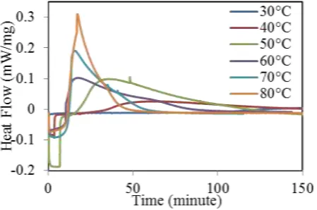
The measurement of the heat evolved during the curing reaction was conducted by means of a TA Instruments DSC Q2000 apparatus. The DSC analysis provided the heat flow versus time and temperature data (Fig. 1 and Fig. 2). To investigate the ultimate heat of the reaction (𝐻𝑈), the heat

flow was measured for the heating ramps of 3°C, 5°C, 10°C and 20°C for the samples weighing 7mg (±0.1) until 250°C (Fig. 1).

Fig.1: Dynamic DSC test results

The isothermal tests were performed at the temperatures of 30°C, 40°C, 50°C, 60°C, 70°C and 80°C (Fig. 2) for the samples weighing 7mg (±0.1) until no further changes in the data can be observed.

3.2.Viscosity Analysis

The viscosity of the Crystic 701 resin with 1% MEKP catalyst as a function of time at room temperature was determined by ICI viscometer. The procedure of the viscosity measurement was i) 100 grams of Crystic 701 in a gelation timer cup was placed in a water bath maintained at a temperature of 25°C, then 1% catalyst was added and stirred into the resin for 30 seconds, ii) an initial sample of resin was taken and the viscosity was measured using an ICI viscometer until the resin had gelled.

3.3.Vacuum Infusion

3.3.1 Flow Monitoring

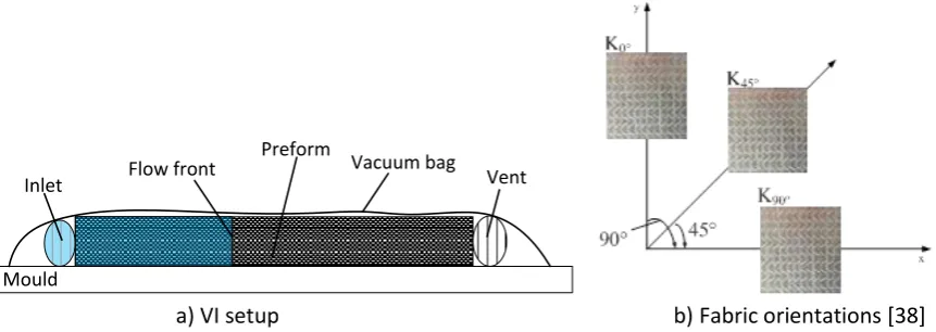
A VI experiment was performed to find out a typical infusion time. The preform consisted of twelve layers non-crimp glass fabric preform (areal weight of 817 g/m2 _{and dimensions of 45cm (flow} direction) x 15cm). Due to the inhomogeneity of the fabric structure, the preform involving all the fabric layers in 0˚ orientation was chosen from [38]. Unlike the standard VI procedure, the distribution medium and the peel ply were not included in the experiment to extend the infusion time. The flow front advancement was monitored using a high-resolution webcam. The details of the flow front monitoring methodology can be found in [38].

Mould

Vacuum bag Preform

Inlet Flow front Vent

a) VI setup b) Fabric orientations [38] Fig. 3: Vacuum infusion experimental procedure

3.3.2. Cure Monitoring

4. Results 4.1.DSC Results

The total isothermal heat of reactions (𝐻𝑇) calculated using the data in Fig. 2 and the ultimate heat

of reactions (𝐻𝑈) calculated using the data in Fig. 1 are presented in Table 2 and Table 3, respectively.

It can be seen that 𝐻𝑈was around 256 J/g (Table 2) and did not depend on the heating rate.

Table 2: Total isothermal heat of reaction

Temperature (°C) 30 40 50 60 70 80

𝐻_𝑇 (J/g) 124 187 234 240 251 254

Table 3: Ultimate heat of reaction of UP resin at different heating rates

Heating Rate (°C/min) 3 5 10 20 Average S.D.

𝐻𝑈 (J/g) 255 261 255 254 256 3

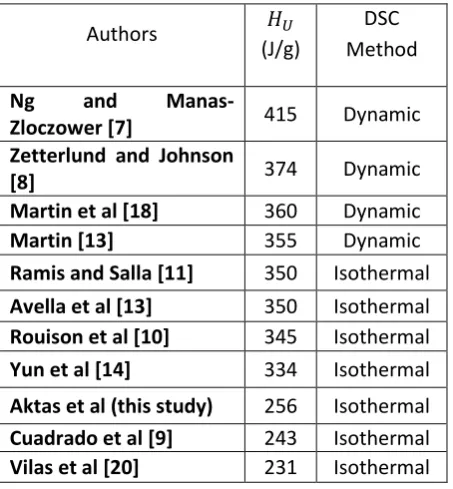
It can be seen that the 𝐻𝑈 found in this study is in the range of the previously reported values (Table

4). The differences in 𝐻𝑈 could be attributed to the individual materials and their contents in the

unsaturated polyester resin, such as catalyst, inhibitors, styrene and other additives.

Table 4: Previously reported studies for unsaturated polyester resins

Authors 𝐻𝑈

(J/g)

DSC Method

Ng and

Manas-Zloczower [7] 415 Dynamic

Zetterlund and Johnson

[8] 374 Dynamic

Martin et al [18] 360 Dynamic

Martin [13] 355 Dynamic

Ramis and Salla [11] 350 Isothermal

Avella et al [13] 350 Isothermal

Rouison et al [10] 345 Isothermal

Yun et al [14] 334 Isothermal

Aktas et al (this study) 256 Isothermal

Cuadrado et al [9] 243 Isothermal

Vilas et al [20] 231 Isothermal

Fig. 4: Conversion profiles as a function of time at different isothermal temperatures

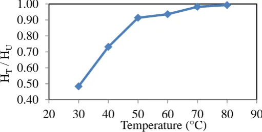
A graph of experimentally determined values of 𝐻𝑇/𝐻𝑈 versus temperature (T) is shown in Fig. 5.

From Eq. 9 in Section 2.1, the ratio of 𝐻𝑇/𝐻𝑈 rose with temperature and was approximated by a

piece-wise linear function of temperature as expressed by Eq. 18. The 𝐻𝑇/𝐻𝑈 data was linear until

50°C and almost levelled off after 50°C.

Fig. 5: HT/HU versus isothermal temperature

𝐻𝑇

𝐻𝑈= {0.0215 𝑇(℃) − 0.1496 𝑇 ≤ 50℃ ~1 𝑇 > 50℃} (18)

4.2. Curve Fittings and Cure Model

The procedure of the application of the empirical autocatalytic cure model to the experimental data and the determination of the constants k, m and n were as follows:

 𝑑𝛽/𝑑𝑡 data were calculated by Eq. 6 using experimentally determined values of 𝑑𝛼/𝑑𝑡 and

HT/HU and plotted against the isothermal conversions 𝛽 (Fig.6),

 The 𝑑𝛽/𝑑𝑡 versus 𝛽 values were curve-fitted with a least-square curve fitting method using

the autocatalytic kinetic model (incorporating the Arrhenius law) and the Levenberg-Marquardt algorithm in MATLAB.

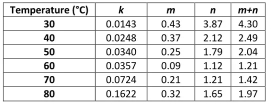
 The constants (Table 5) were obtained as the results of the curve fittings.

0.40

0.50

0.60

0.70

0.80

0.90

1.00

20

30

40

50

60

70

80

90

H

/

H

The fittings (Fig. 6) were in good agreement with the isothermal rate of degree of cure (𝑑𝛽/𝑑𝑡) versus degree of cure (𝛽) data for each isothermal case.

a) 30°C b) 40°C

c) 50°C d) 60°C

e) 70°C f) 80°C

Fig. 6: Autocatalytic model fittings on the experimental 𝑑𝛽/𝑑𝑡 versus 𝛽 data

Table 5: Cure kinetic parameters

Temperature (°C) k m n m+n

30 0.0143 0.43 3.87 4.30

40 0.0248 0.37 2.12 2.49

50 0.0340 0.25 1.79 2.04

60 0.0357 0.09 1.12 1.21

70 0.0724 0.21 1.21 1.42

80 0.1622 0.32 1.65 1.97

0 0.1 0.2 0.3 0.4

1 2 3 4 5

x 10-5

Degree of Cure

Rate of Degree of Cure (dB/dt) Isothermal (30°C) Curve fitting (R-square: 0.95 )

0 0.1 0.2 0.3 0.4 0.5 0.6 0.7

2 4 6 8 10 12 14

x 10-5

Degree of Cure

Rate of Degree of Cure (dB/dt)

Isothermal (40°C ) Curve fitting (R-square: 0.98)

0 0.1 0.2 0.3 0.4 0.5 0.6 0.7 0.8

0 0.5 1 1.5 2 2.5

x 10-4

Degree of Cure

Rate of Degree of Cure (dB/dt)

Isothermal (50°C ) Curve fitting (R-square: 0.96)

0 0.2 0.4 0.6 0.8

0 1 2 3 4

x 10-4

Degree of Cure

Rate of Degree of Cure (dB/dt)

Isothermal (60°C )

Curve fitting (R-square: 0.97)

0 0.2 0.4 0.6 0.8

0 2 4 6

8x 10

-4

Degree of Cure

Rate of Degree of Cure (dB/dt)

Isothermal (70°C ) Curve fitting (R-square: 0.99

0 0.2 0.4 0.6 0.8 1

0 2 4 6 8 10 12

x 10-4

Degree of Cure

Rate of Degree of Cure (dB/dt) Isothermal (80°C)

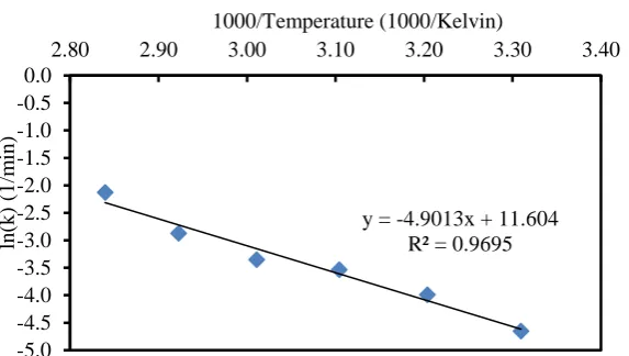
With the modification of Eq.13, Eq. 19 representing a linear correlation between 𝑙𝑛𝑘 and 1/𝑇 can be obtained to find out the activation energy and the pre-exponential factor A. Fig. 7 shows this linear relationship with an R2 _{of 0.9695.}

𝑙𝑛𝑘 = 𝑙𝑛𝐴 − 𝐸/𝑅𝑇 (19)

Fig. 7: Logarithm of the rate constant k as a function of reciprocal absolute temperature

From Eq. 19 and Fig. 7, the pre-exponential factor (A) and the activation energy (E) were found as 109098 1/min and 40.73 kJ/mol, respectively. From here, the following final cure kinetics expression for Crystic 701 resin with 1% MEKP content was obtained:

𝑑𝛽

𝑑𝑡 = (109098 ∗ 𝑒𝑥𝑝 (

−40730 8.31∗𝑇)) ∗ 𝛽

𝑚_{(1 − 𝛽)}𝑛 ₍₂₀₎

In Eq. 20, 𝑚 and 𝑛 are the temperature dependent reaction orders. In this study, in order to find a representative expression between the isothermal conditions, they were represented in the form of a second-order polynomial expression. The relationships between the constants 𝑚, 𝑛 and reciprocal temperatures (Fig. 8) were expressed by second order polynomial curves, represented by Eq. 21 and Eq. 22 for 𝑛 and 𝑚, respectively.

Fig. 8: Reaction orders m and n as a function of reciprocal absolute temperature

𝑛 = 17.211 (1

𝑇) 2

− 101.53 (1

𝑇) + 150.78 (21)

y = -4.9013x + 11.604 R² = 0.9695

-5.0 -4.5 -4.0 -3.5 -3.0 -2.5 -2.0 -1.5 -1.0 -0.5 0.0

2.80 2.90 3.00 3.10 3.20 3.30 3.40

ln (k ) (1 /m in ) 1000/Temperature (1000/Kelvin)

y = 1.7572x2_{- 10.462x + 15.678}

R² = 0.7403

y = 17.211x2_{- 101.53x + 150.78}

R² = 0.9648

0.0 0.5 1.0 1.5 2.0 2.5 3.0 3.5 4.0

2.80 3.00 3.20 3.40

m

,n

1000/Temperature (1000/Kelvin)

𝑚 = 1.7572 (1_𝑇)2− 10.462 (1_𝑇) + 15.678 (22)

4.3.Vacuum Infusion

The flow front advancement versus time curve (total filling time of 4430 seconds) is demonstrated in Fig. 9, and compared with the viscosity (as a function of time) data. It can be seen that the viscosity was around 0.19 Pa*s during the infusion of the 0° oriented preform. The viscosity remained almost constant up to 12000 seconds (~3.5 hours). The resin gelled around 14000 seconds (~4 hours) and it was not processable (Fig. 9 and Fig. 13).

Fig. 9: The filling times and the viscosity data comparison [38]

The temperature monitoring results during and after the infusion process is presented in Fig. 11a and Fig. 11b, respectively. It can be seen that the temperature inside the laminate was more stable than the ambient temperature due to being sealed by the preform. In Fig. 11a, stage-1, stage-2 and stage-3 represent the dry (before the infusion), the wetting and the wetted stages, respectively. The entire room temperature cure monitoring data is presented in Fig. 11b. Apart from the exothermic reaction temperature, which was the peak point around 4 hours, the general temperature trend inside the laminate was similar to the ambient temperature trend, but it was slightly higher due to the on-going curing reactions and the stability.

ambient and the laminate. The time of the peak temperature determined by the in-built thermocouple (Fig. 11b) and the gelling time of the resin (Fig.9) determined by the viscometer were same (4 hours).

4.4. Numerical Simulation and Validation

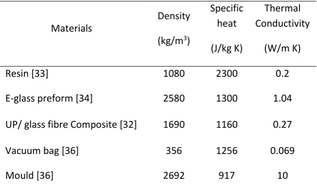
In the numerical study, the cure and the temperature changes during and after the filling process were studied and compared with the experimental results. The simulation study included i) the material properties (Table 6) and the boundary conditions (ambient temperature=29°C, initial resin and mould pressure=29°C), ii) the resin flow simulation inputs of the 0° oriented twelve layer preform infusion case (inlet pressure=1atm, outlet pressure=0 atm, the average porosity=0.5, the average permeability values in x and y directions and the permeability orientations on the mesh) adapted from [38] in order to obtain a typical filling time for this study, iii) the experimental viscosity data as a function of time (Fig. 9), iv) the enthalpy of 256 J/g (Table 3) and v) the final autocatalytic cure kinetics expression (Eq. 20). The flow simulation details were not the focus of this study and the details can be found in [38]. The cure simulation time was set to 24 hours in addition to the total wetting time of 4432 seconds. Fig.10 illustrates the representation of the fabric layers, the vacuum bag and the mould using the solid elements.

Table 6: Properties of the materials

Materials

Density (kg/m3₎

Specific heat (J/kg K)

Thermal Conductivity

(W/m K)

Resin [33] 1080 2300 0.2

E-glass preform [34] 2580 1300 1.04

UP/ glass fibre Composite [32] 1690 1160 0.27

Vacuum bag [36] Mould [36]

356 2692

1256 917

0.069 10

Vacuum bag

Mould

Fig.10: Illustration of the zones in the simulation (Thicknesses, vacuum bag: 0.5mm, mould: 5mm and each fabric layer: 1mm)

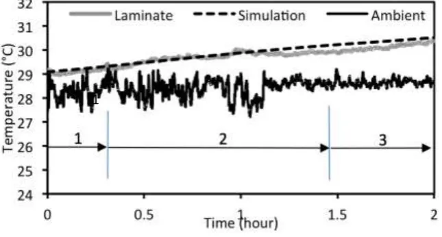
Fig. 11 presents the comparison of the numerical and the experimental temperature data. In Fig. 11a, Stage-1, Stage-2 and Stage-3 represents the temperatures i) before the filling, ii) during the filling (duration of ~1 hour) and iii) after the filling, respectively. It can be seen that the temperature prediction well agreed with the experimental data in the first 2 hours. In Fig. 11b, the overall numerical temperature pattern (including Stage-1, Stage-2 and Stage-3) was similar to the experimentally measured data. The peak temperature times for the experimental and the numerical were around 4 and 4.5 hours, respectively.

a) Temperature variation up to 2 hours (1: dry, 2: during filling, 3: after filling)

b) Temperature monitoring during the room temperature curing Fig. 11: Experimental and numerical temperature results

Fig. 12 presents the cure, the temperature and the filling time results. The filling time (the total time of 4432 seconds) was simulated according to the resin flow simulation inputs reported in [38] using the same materials and the boundary conditions. The simulation results (Fig. 12) of the cure and the temperature from the inlet to the vent were from the moment of 4432 seconds once the resin

reached the vent. The cure was between 0 and 0.05, and the temperature was between 28.5°C and 30°C.

Fig.12: Cure (0: uncured and 1: cured), temperature (°C) and filling time (second) distribution

Fig. 13: Comparison of the autocatalytic model results with the experimental DSC cure data and viscosity data

4. Conclusion

This paper focused on the cure kinetics (based on the DSC method), the cure modelling (using the autocatalytic cure kinetics model), and the process cure simulation (in PAM-RTM) studies. A representative slow and room temperature curing thermoset resin system (Crystic 701 with 1% MEKP catalyst) for the VI process was used in the experiments.

From the literature review, it was seen that the DSC is a reliable method to study the cure kinetics of thermosets. The isothermal and the dynamic tests were performed to find out the total isothermal heat of reaction and the ultimate heat of reaction results. The ultimate heat of reaction did not depend on the heating rate and it was found as 256 J/g. The total heat of reaction also enabled the calculation of the conversion profiles. The autocatalytic empirical cure kinetics model incorporating the Arrhenius equation was applied to the rate of degree of cure versus degree of cure curves of each isothermal test, and good agreement was found. Then, the temperature dependants of the model (m, n and k), and a final equation representing the cure behaviour of the UP resin were obtained.

The aim of the cure kinetics study was to provide the key inputs for the cure simulation, such as the enthalpy, the cure model, and the temperature dependant coefficients. The degree of cure and the temperature change during and after the filling stage were obtained from the simulation. Even though the cure simulation result was not as accurate as the DSC cure data (measured for 24 hours at room temperature), the cure behaviour was representative and both results were comparable. The cure simulation result was in good agreement in the first 2 hours with the experimental DSC cure data, and the final degree of cure prediction was very close to the DSC. The resin was processable up to 4 hours according to the viscosity measurement.

the preform, the mould and the vacuum bag, the exothermic peak temperature was only 4°C higher than the ambient temperature.

The parameters of this study can be used for more realistic vacuum infusion cases with Crystic 701 resin system. Also, the cure kinetics of other thermoset resin systems can be investigated through the steps of this study to model the cure behaviour and to aid the VI process simulations of large structures.

Acknowledgements

This project is supported by the EPSRC project: EP/H020926/1. The authors would like to acknowledge Scott Bader for providing the Crystic 701 resin system, and ESI group for the PAM-RTM software.

References

[1] Ton-That MT, Cole KC, Jen CK, Franca DR. Polyester cure monitoring by means of different techniques. Polymer Composites, vol. 21, no.4, p.605-618, August 2000.

[2] Um MK, Daniel IM, Hwang BS. A study of cure kinetics by the use of dynamic differential scanning calorimetry. Composites Science and Technology, 62, p.29-40. 2002.

[3] Karkanas PI, Partridge IK, Attwood D. Modelling the cure of a commercial epoxy resin for applications in resin transfer moulding. Polymer International, 41, p.183- 191, 1996.

[4] Rabearison N, Jochum Ch, Grandidier JC. A cure kinetics, diffusion controlled and temperature dependent, identification of the Araldite LY556 epoxy. Journal of Material Science, DOI 10.1007/s10853-010-4815-7

[5] Lee WI, Loos AC, Springer GS. Heat of reaction, degree of cure, and viscosity of Hercules 3501-6 Resin. Journal of Composite Materials, vol. 16, p.510-520,1982.

[6] Sourour S, Kamal MR. Differential scanning calorimetry of epoxy cure: isothermal cure kinetics. Thermochimica Acta, 14, p.41-59, 1976.

[7] NG H, Manas-zloczower. A nonisothermal differential scanning calorimetry study of the curing kinetics of an unsaturated polyester system. Polymer Engineering and Science. Vol. 29, Issue 16, p.1097-1102. August 1989. DOI: 10.1002/pen.760291604

[8] Zetterlund PB, Johnson AF. A new method for the determination of the Arrhenius constants for the cure process of unsaturated polyester resins based on a mechanistic model. Thermocimica Acta, Volume 289, p.209-221, 1996.

[10] Rouison D, Sain M, Couturier M. Resin transfer moulding of natural fibre reinforced plastic. I. Kinetic study of an unsaturated polyester resin containing an inhibitor and various promoters. Journal of Applied Polymer Science, vol. 89, p.2553-2561, 2003.

[11] Ramis X, Salla JM. Effect of the inhibitor on the curing of an unsaturated polyester resin. Polymer, vol. 36, no.18, pp.3511-3521, 1995.

[12] Avella M, Martuscelli E, Mazzola M. Kinetic study of the cure reaction of unsaturated polyester resins. Journal of Thermal Analysis, vol.30, p.1359-1366. 1985.

[13] Martin JL. Kinetic analysis of two DSC peaks in the curing of an unsaturated polyester resin catalysed with methylethylketone peroxide and cobalt octoate. Polymer Engineering and Science, DOI 10.1002/pen.20667. 2007.

[14] Yun YM, Lee SJ, Lee KJ, Lee YK, Nam JD. Composite cure kinetic analysis of unsaturated polyester free radical polymerisation. Journal of Polymer Science: Part B: Polymer Physics, vol.35, p.2447-2456. 1997.

[15] Boyard N, Sinturel C, Vayer M, Erre R. Morphology and cure kinetics of unsaturated polyester resin/block copolymer blends. Journal of Applied Polymer Science, vol.102, p.149-165. 2006.

[16] Yousefi A. Lafleur PG, Gauvin R. The effects of cobalt promoter and glass fibres on the curing behaviour of unsaturated polyester resin. Journal of Vinyl Additives Technology. Vol.3, no. 2, p.157-169. June 1997.

[17] Yousefi A, Lafleur PG, Gauvin R. Kinetic studies of thermoset cure reactions: a review. Polymer Composites, vol. 18, no.2, April 1997.

[18] Martin JL, Cadenato A, Salla JM. Comparative studies on the non-isothermal DSC curing kinetics of an unsaturated polyester resin using free radicals and empirical models. Thermochimica Acta, 306, p.115-126. 1997.

[19] Gao J, Dong C, Du Y. Nonisothermal curing kinetics and physical properties of unsaturated polyester modified with EA-POSS. International Journal of Polymeric Materials, 59, p.1-14, 2010. [20] Vilas JL, Laza JM, Garay MT, Rodriguez M, Leon LM. Unsaturated polyester resins cure: Kinetic, rheologic, and mechanical-dynamical analysis. I. Cure Kinetics by DSC and TSR. Journal of Applied Polymer Science. Vol.79, p.447-457. 2001.

[21] Laurent-Mounier A, Binetruy C, Krawczak P. Multipurpose carbon fibre sensor design for analysis and monitoring of the resin transfer moulding of polymer composites. Polymer Composites, DOI 10.1002/pc.20104, 2005.

[22] Eum SH, Kageyama K, Murayama H, Uzawa K, Ohsawa I, Kanai M, Kobayashi S, Igawa H, Shirai T. Structural health monitoring using fibre optic distributed sensors for vacuum-assisted resin transfer moulding. Smart Materials and Structures, 16, p.2627-2635, 2007.

[24] Bang KG, Kwon JW, Lee DG, Lee, JW. Measurements of the degree of cure of glass fibre-epoxy composites using dielectrometry. Journal of Materials Processing Technology, 113, p.209-214, 2001. [25] Kobayashi S, Matsuzaki R, Todoroki A. Multipoint cure monitoring of CFRP laminates using a flexible matrix sensor. Composites Science and Technology, 69, p.378-384, 2009.

[26] Chiu HT, Yu B, Chen SC, Lee LJ, Heat transfer during flow and resin reaction through fibre reinforcement. Chemical Engineering Science, 55, p.3365-3376, 2000.

[27] Rouison D, Sain M, Couturier M. Resin transfer moulding of natural fibre reinforced composites: cure simulation. Composites Science and Technology, 64, p.629-644, 2004.

[28] Michaud DJ, Beris AN, Dhurjati PS. Curing behaviour of thick sectioned RTM composites. Journal of Composite Materials, vol. 32, no.14, p.1273-1296, 1998.

[29] Kiuna N, Lawrance CJ, Fontana QPV, Lee PD, Selerland T, Spelt PDM. A model for resin viscosity during cure in the resin transfer moulding process. Composites Part A: Applied Science and Manufacturing, 33, p.1497-1503, 2002.

[30] Blest DC, Duffy BR, McKee S, Zulkifle AK. Curing simulation of thermoset composites. Composites: Part A: Applied Science and Manufacturing,, 30, p.1289-1309, 1999.

[31] Hickey CMD, Bickerton S. Cure kinetics and rheology characterisation and modelling of ambient temperature curing epoxy resins for resin infusion/VARTM and wet layup applications. Journal of Materials Science, DOI 10.1007/s10853-012-6781-8, 2012.

[32] Hsiao KT, Little R, Restrepo O, Bob M. A study of direct cure kinetic characterisation during liquid composite moulding. Composites: Part A: Applied Science and Manufacturing, 37, p.925-933, 2006.

[33] Crystic Composites Handbook. Scott Bader

[34] Schuster J, Heider D, Sharp K, Glowania M. Thermal conductivities of three-dimensionally woven fabric composites. Composites Science and Technology. DOI:10.1016/j.compscitech.2008.03.024. 2009.

[35] Dusi MR, Lee WI, Ciriscioli PR, Springer GS. Cure kinetics and viscosity of Fiberite 976 resin. Journal of Composite Materials, 27, p.243-261, 1987.

[36] Joshi SC, Liu XL, Lam YC. A numerical approach to the modelling of polymer curing in fibre-reinforced composites. Composites Science and Technology, 59, p.1003-1013.

[37] Blest DC, McKee S, Zulkifle AK, Marshall P. Curing simulation by autoclave resin infusion. Composites Science and Technology, 59, p.2297-2313, 1999.