An Improved Modular Modeling for Analysis of Closed-Cycle Absorption Cooling Systems

AN IMPROVED MODULAR MODELING FOR ANALYSIS OF

CLOSED-CYCLE ABSORPTION COOLING SYSTEMS

K. Abbaspour-Sani*, H. R. Haghgoo and F. Bahar

Materials and Energy Research Center P.O. Box 31787-316, Karaj, Iran

[email protected] - [email protected] - [email protected]

*Corresponding Author

(Received: February 24, 2007 - Accepted in Revised Form: November 22, 2007)

Abstract A detailed modular modeling of an absorbent cooling system is presented in this paper.

The model including the key components is described in terms of design parameters, inputs, control variables and outputs. The model is used to simulate the operating conditions for estimating the behavior of individual components and system performance and to conduct a sensitivity analysis based on the given control variables. The proposed model has been validated by means of comparing the predicted results with the experimental data in a full-scale absorbent cooling system installed at MERC. Careful attention was given to estimate the behavior of the system at transient mode. Based on operating conditions, a range of time-constant start-up time had been estimated for generator and evaporator. The results indicated that the model predictions were in good agreement with experimental data. Sensitivity analysis also showed that the performance characteristics of the system could be approximated by generalized polynomial functions of order 2 in terms of control variables. Finally typical performance results are discussed.

Keywords Closed-Cycle Absorption Cooling System, Modular Modeling, Simulation,

Performance Characteristics, Transient Mode

ﻩﺪﻴﻜﭼ

ﺵﻭﺭﻪﻟﺎﻘﻣﻦﻳﺍﺭﺩ ﻲﻣﻪﺋﺍﺭﺍﻞﻴﺼﻔﺗﻪﺑﻲﺑﺬﺟﺪﻳﺮﺒﺗﻢﺘﺴﻴﺳﻚﻳﻱﺍﺮﺑﺀﺰﺟﻪﺑﺀﺰﺟﻱﺯﺎﺳﻮﮕﻟﺍ

ﺩﻮﺷ . ﻦﻳﺍ

ﻢﺘﺴﻴﺳﻲﻠﺻﺍﻱﺍﺰﺟﺍ ﻞﻣﺎﺷﻪﻛﻮﮕﻟﺍ )

ﺏﺬﺟ،ﻲﺗﺭﺍﺮﺣﺪﻟﻮﻣ ،ﻩﺪﻨﻨﻛﺮﻴﺨﺒﺗ،ﻩﺪﻨﻟﺎﮕﭼ ﻲﺗﺭﺍﺮﺣﻝﺪﺒﻣ ﻭﻩﺪﻨﻨﻛ

( ،ﺖﺳﺍ

ﻲﻣﻒﻳﺮﻌﺗﻢﺘﺴﻴﺳﻲﺟﻭﺮﺧﻭﻝﺮﺘﻨﻛﻞﺑﺎﻗﻱﺎﻫﺮﻴﻐﺘﻣ،ﻱﺩﻭﺭﻭ ﻲﺣﺍﺮﻃﻱﺎﻫﺮﺘﻣﺍﺭﺎﭘ ﺐﺴﺣﺮﺑ ﺩﻮﺷ

. ﻣﺍﺭﻮﮕﻟﺍ ﻲ ﻥﺍﻮﺗ

ﻪﻴﺒﺷﻱﺍﺮﺑ ﺑﻢﺘﺴﻴﺳﺭﺎﻛﻂﻳﺍﺮﺷﻱﺯﺎﺳ ﻪ

ﺁﺭﺎﻛﺩﺭﻭﺁﺮﺑﻭﻦﻴﻤﺨﺗﺭﻮﻈﻨﻣ ﻳ

ﺁﺭﺎﻛ،ﻢﺘﺴﻴﺳﻱﺍﺰﺟﺍﻪﻧﺎﮔﺍﺪﺟﺭﺎﺘﻓﺭﻲ ﻳ

ﻞﻛﻲ

ﺁﺭﺎﻛﺖﻴﺳﺎﺴﺣﻞﻴﻠﺤﺗﻱﺍﺮﺑﺰﻴﻧﻭﻢﺘﺴﻴﺳ ﻳ

ﻪﺑﻢﺘﺴﻴﺳﻲ ﺩﺮﺑﺭﺎﻜﺑﻝﺮﺘﻨﻛﻞﺑﺎﻗﻱﺎﻫﺮﻴﻐﺘﻣ

. ﻪﺴﻳﺎﻘﻣﺎﺑﻮﮕﻟﺍﻱﺯﺎﺳﺮﺒﺘﻌﻣ

ﺶﻴﭘ ﺞﻳﺎﺘﻧ ﺖﺳﺪﺑ ﻲﺑﺮﺠﺗ ﺕﺎﻋﻼﻃﺍﻭﻩﺪﺷﻲﻨﻴﺑ

ﺯﺍﻩﺪﻣﺁ ﻲﺑﺬﺟﺪﻳﺮﺒﺗ ﻢﺘﺴﻴﺳﻚﻳ ﺶﻳﺎﻣﺯﺁ )

ﺐﺼﻧ ﺖﻳﺎﺳﺭﺩﻩﺪﺷ

ﻱﮊﺮﻧﺍﻭ ﺩﺍﻮﻣ ﻩﺎﮕﺸﻫﻭﮋﭘ (

ﻪﺘﻓﺮﻳﺬﭘ ﺕﺭﻮﺻ

ﺖﺳﺍ . ﻦﻳﺍ ﺭﺩ ،ﻖﻴﻘﺤﺗ ﺮﺘﺸﻴﺑ ﻪﺟﻮﺗ ﯼ

ﺶﻴﭘ ﻪﺑ ﺭﺩ ﻢﺘﺴﻴﺳ ﺭﺎﺘﻓﺭ ﻲﻨﻴﺑ

ﻂﻳﺍﺮﺷﺐﺴﺣﺮﺑﻭﻩﺪﻳﺩﺮﮔﺭﺍﺪﻳﺎﭘﺎﻧﺖﻟﺎﺣ

ﻢﺘﺴﻴﺳﺭﺎﻛ ،

ﻩﺍﺭ ﻥﺎﻣﺯﻱﺍﺮﺑﻱﺩﻭﺪﺣ ﻩﺪﻨﻨﻛﺮﻴﺨﺒﺗﻭﻲﺗﺭﺍﺮﺣﺪﻟﻮﻣﻱﺯﺍﺪﻧﺍ

ﻩﺪﺷﻦﻴﻴﻌﺗ

ﺖﺳﺍ . ﺘﻧ ﻲﻣﻥﺎﺸﻧﻞﺻﺎﺣﺞﻳﺎ ﺶﻴﭘﻪﻛﺪﻫﺩ

ﻱﺭﻮﻃﻪﺑﺩﺭﺍﺩﺖﻘﺑﺎﻄﻣﻲﺑﻮﺧﻪﺑﻲﺑﺮﺠﺗﺞﻳﺎﺘﻧﺎﺑﻮﮕﻟﺍﻲﻨﻴﺑ

ﻲﻣﺍﺭﻮﮕﻟﺍﻦﻳﺍﻪﻛ ﺩﺎﻳﺯﺖﻗﺩﺎﺑﻥﺍﻮﺗ

ﯼﺍﺮﺑ ﻪﻴﺒﺷ ﻢﺘﻴﺳﻱﺯﺎﺳ ﺩﺮﺑﺭﺎﻜﺑﻪﺘﺴﺑﺭﺍﺪﻣﺎﺑﻲﺑﺬﺟﺪﻳﺮﺒﺗﻱﺎﻫ

. ﺞﻳﺎﺘﻧﻦﻴﻨﭽﻤﻫ

ﻲﻣﻥﺎﺸﻧﻝﺮﺘﻨﻛﻞﺑﺎﻗﻱﺎﻫﺮﻴﻐﺘﻣﻪﺑﻢﺘﺴﻴﺳﺖﻴﺳﺎﺴﺣﻞﻴﻠﺤﺗﻪﻌﻟﺎﻄﻣﺯﺍﻞﺻﺎﺣ ﺪﻫﺩ

ﻪﺼﺨﺸﻣﻪﻛ ﺁﺭﺎﻛﻱﺎﻫ

ﻳ ﻢﺘﺴﻴﺳﻲ

ﻲﻣ ﺍﺭ ﻪﻠﻤﺟﺪﻨﭼ ﻪﻄﺑﺍﺭ ﻚﻳ ﺎﺑ ﻥﺍﻮﺗ ﻂﻳﺍﺮﺷ ﺭﺩ ﺎﻫﺮﻴﻐﺘﻣ ﻦﻳﺍ ﺐﺴﺣﺮﺑ ﻡﻭﺩ ﻪﺒﺗﺮﻣ ﺯﺍ ﻱﺍ

ﺩﻮﻤﻧ ﺐﻳﺮﻘﺗ ﻢﺘﺴﻴﺳ ﺭﺎﻛ .

ﻪﻟﺎﻘﻣﻦﻳﺍﺭﺩﻩﺮﺧﻻﺎﺑ ﯽﻳﺎﻫﻪﻧﻮﻤﻧ

ﺖﺳﺪﺑﺞﻳﺎﺘﻧﺯﺍ

ﻲﻣﺭﺍﺮﻗﻲﺳﺭﺮﺑﻭﺚﺤﺑﺩﺭﻮﻣﻩﺪﻣﺁ ﺪﻧﺮﻴﮔ

.

1. INTRODUCTION

Over the past few decades considerable research has been devoted to the development of absorbent refrigeration systems and their performance prediction. At the same time, there have been other researches underway for the advanced absorption cycles and non-conventional working fluids, which can provide significantly greater efficiency than

A computer simulation has been conducted to analyze a water-LiBr, water absorption heat pump [5,6]. The code is a system-oriented program with a structure that does not allow easy modification to model other systems. Based on specified design parameters, the code calculates the operating parameters of the system for a variety of conditions. A modular simulation was also conducted to analyze closed-cycle systems with different working fluid and under steady state conditions [7]. The code has been modified by adding some subroutines to make the analysis of open-cycle systems possible [8].

As a result the on-off control strategy most commonly used in residential applications for the cooling system, often calls for cooling when the room temperature rises above a set point and shuts off below the set point. If the cooling capacity is significantly greater than the building-cooling load, the thermostat will cycle and cooling system will spend part of its operating time in a transient mode [9].

This paper describes the performance analysis of a closed-cycle absorption system during its operation. The analysis was performed using a code developed for modular simulations of absorption system under varying operating modes. Based on design parameters and control variables, the code evaluates the start up time and temperature profile in the generator during the warm up period. It also fixes the variable parameters for prescribed conditions and finally computes the operating parameters. The present work, attempts to predict the performance of the system and of its main components.

2. DESCRIPTION OF EXPERIMENTAL SYSTEM

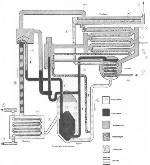
Figure 1 schematically describes the absorbent cooling system investigated in this study. It consists of an evaporator, an absorber, a generator, a recuperative heat exchanger and a water-cooled condenser. The number in a circle, as shown in Figure 1, indicates the fluid state point. Liquid refrigerant is supplied at state point (8) to the evaporator, where its evaporation is used to chill the entering airflow with entering

temperature as state (5) and leaving at (6). The liquid refrigerant entering the evaporator at state (8) reaches its evaporation temperature and leaves the evaporator at state (7). The vapor is absorbed in the absorber by a weak Li-Br water solution entering at state (12), reaching equilibrium and leaving strong solution at state (14). The heat of absorption is rejected to a flow of cooling water entering at state (1) and leaving the condenser at state (2). The strong solution is circulated through the heat exchanger to the generator at state (17) where it is heated by a hot water stream. The regenerated solution at state (12) is returned to the absorber through the heat exchanger.

3. MATHEMATICAL MODEL

3.1. Transient Mode

When the cooling system

is warmed up, the Li-Br water solution will begin circulating between the generator and the absorber. No vapor will evolve unless the generator and all the solution held up in the generator have been heated up to a minimum temperature (Tmin). This

temperature is the boiling point of the Li-Br solution whose concentration corresponds to the chiller’s initial charge, at a pressure set by the condenser temperature.

If the generator sensible heat exchanger and the absorber are all modeled as constant effectiveness heat exchangers during the warm up and the generator is considered as a single node thermal capacitance; and if it is assumed that the absorber and sensible heat exchanger respond much more rapidly than the generator, then the generator temperature during startup will vary exponentially [9] as:

H

τ τ

-e ) ss , g T o , g T ( ss , g T g

T = + − (1)

Where Tg,o and Tg,ss are the initial and steady state

generator temperature, respectively.

Figure 1. Schematic diagram for experimental system.

evaporator temperature is assumed constant and the cooling capacity and coefficient of performance are empirical functions in terms of the

generator and condensing water temperatures. When the generator temperature is above Tmin, then

⎪ ⎩ ⎪ ⎨ ⎧ ⎟ ⎠ ⎞ ⎜ ⎝ ⎛ = ⎟ ⎠ ⎞ ⎜ ⎝ ⎛ = ≥ cw T , g T 2 f g Q cw T , g T 1 f e Q min T g T

if (2)

When the generator temperature is less than Tmin,

the following would then apply:

( )

⎪⎩ ⎪ ⎨ ⎧ ⎟ ⎠ ⎞ ⎜ ⎝ ⎛ = = g T -s T g UA g Q 0 e Q min T g T

if p (3)

3.2. Steady State Mode

In order to simulate the cooling system, physical models for the system components should be derived. Due to the complex nature of simultaneous heat and mass transfer process, occurring in various components of the cooling system, physical models developed to date, have all been incorporated with various simplifying assumptions [2,8]. These physical models representing the water condenser, evaporator, absorber, heat exchanger and generator are described in details in this section. These models are generally based on the same physical laws applied for system components (mass and energy balance equations):

3.2.1. Water cooled condenser The condenser

as illustrated schematically in Figure 1, consists of a shell and tube heat exchanger. The cooling water stream entering the tubes and cools the refrigerant steam that entering the shell at state point (11) and leaving it at (8). The following equation applies: ⎟ ⎠ ⎞ ⎜ ⎝ ⎛ ₋ ⎟ ⎠ ⎞ ⎜ ⎝ ⎛ = ⎟ ⎠ ⎞ ⎜ ⎝ ⎛ + ⎟ ⎠ ⎞ ⎜ ⎝ ⎛ ⎟ ⎠ ⎞ ⎜ ⎝ ⎛ = 16 t 2 t cw V p ρC f h -8 h r m 8 t -11 t r p C m c Q & & & (4)

3.2.2. Evaporator According to Figure 1, the

evaporator consists of a coil, in which a stream of air is blown through its external surface. The following equation applies:

⎟ ⎠ ⎞ ⎜ ⎝ ⎛ ₋ ⎟ ⎠ ⎞ ⎜ ⎝ ⎛ρ = ⎟ ⎠ ⎞ ⎜ ⎝ ⎛

= t₅ t₆

a V p C f h -7 h r m e

Q & & (5)

3.2.3. Absorber The evaporator as illustrated

schematically in Figure 1, consists of a cylindrical shell filled with solution and a water coil inside it for rejection of heat. The following equations apply: Energy balance for cooling water:

⎟ ⎠ ⎞ ⎜ ⎝ ⎛ ₋ ⎟ ⎠ ⎞ ⎜ ⎝ ⎛ρ

= t₁₆ t₁₅

cw V p C ab

Q & (6)

Energy balance for the solution:

( )

mh₁₄

( )

mh₁₂ m_rh₇ ab

Q + & = & + & (7)

Mass balance for the solution:

14 m r m 12

m& + & = & (8)

Mass balance for salt in the solution:

( )

m&x₁₂=

( )

m&x₁₄ (9)

Where h and x are the enthalpy of solution and the concentration ratio of salt in the solution, respectively at various state points and can be determined by the approach followed in the Appendix.

3.2.4. Heat exchanger Again, according to

Figure 1 the heat exchanger consists of a shell, protected from heat losses by insulation and an inner shell. Solution to be regenerated enters the inner shell at the top at state (13), flows down and absorbs heat from the weak solution and leaves at state (12). The strong solution enters from state (14) and leaves towards the generator at state (17). The following equation applies:

⎟ ⎠ ⎞ ⎜ ⎝ ⎛ ₋ = ⎟ ⎠ ⎞ ⎜ ⎝ ⎛

=m_r h₁₃-h₁₂ m₁₄ h₁₇ h₁₄ hx

Q & & (10)

3.2.5. Generator A schematic presentation of the

Figure 2. Schematic flow chart for the simulation code. Heat balance for hot water:

⎟ ⎠ ⎞ ⎜

⎝ ⎛ − ⎟

⎠ ⎞ ⎜ ⎝ ⎛

= t₃ t₄

hw V p

ρC g

Q & (11)

Heat balance for generator:

( )

mh₁₇ Q_loss m_rh₁₁ m₁h₁₃ g

Q + & = ++& + & (12)

4. COMPUTER SIMULATION CODE

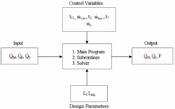
The computer simulation code developed in this study is a modular code such as the one developed by Grossman, et al [7]. Considering that the studied absorption cooling system consists of standard components described in previous section, each of these is simulated by individual subroutines. These subroutines describe the components behavior by implying the mathematical models developed in Section 3. They are linked together in the main program to analyze the whole system.

Figure 2 shows the program flowchart, in which the major variables required to describe the full and part load performance of the absorption cooling system are shown as input, output, design parameters and control variables. The input variables are the thermal energy received from the building at a lower temperature, electrical energy

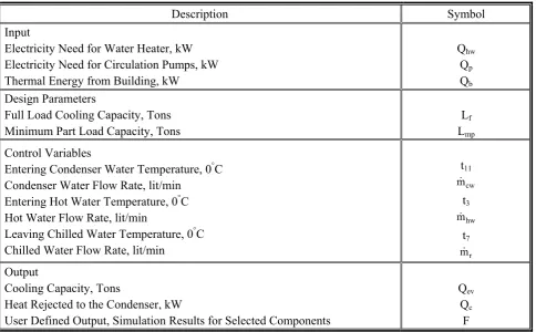
required to provide low-pressure hot water stream and energy required to drive circulation pumps for absorbent and refrigerant. The output contains the heat rejected from the load (cooling capacity), heat rejected from the condenser and the user defined output results, which contain selected components simulations. The design parameters contain the full load and the minimum part load capacities. In order to analyze the system results at different operating conditions, it is necessary to simulate the control variables that affect the performance in order to obtain the maximum COP. These variables are shown in Table 1.

5. EXPERIMENTAL SETUP

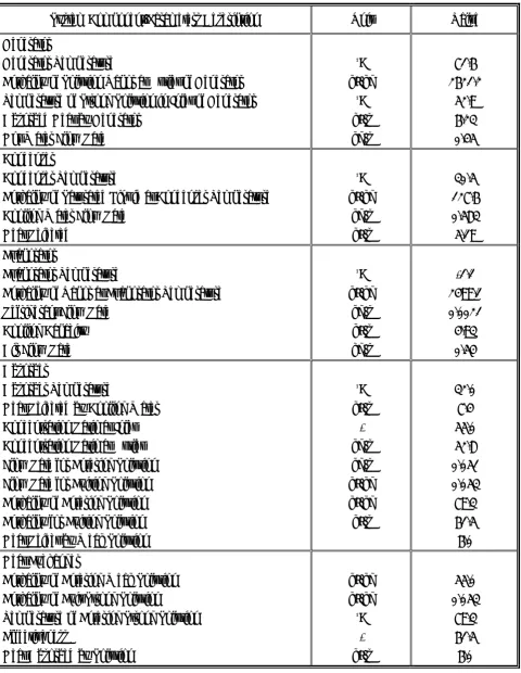
TABLE 1. List of Variables Needed for Analyze of an Absorption Cooling System.

Description Symbol Input

Electricity Need for Water Heater, kW Electricity Need for Circulation Pumps, kW Thermal Energy from Building, kW

Qhw

Qp

Qb

Design Parameters

Full Load Cooling Capacity, Tons Minimum Part Load Capacity, Tons

Lf

Lmp

Control Variables

Entering Condenser Water Temperature, 0°_C

Condenser Water Flow Rate, lit/min Entering Hot Water Temperature, 0°_C

Hot Water Flow Rate, lit/min

Leaving Chilled Water Temperature, 0°_C

Chilled Water Flow Rate, lit/min

t11 cw

m&

t3 hw

m&

t7 r

m&

Output

Cooling Capacity, Tons

Heat Rejected to the Condenser, kW

User Defined Output, Simulation Results for Selected Components

Qev

Qc

F

TABLE 2. Experimental Results for Transient Mode (30th December 1999).

Time From Start Point in Minutes Parameters Need to be Measured

0 5 10 15 20 25 30 35 40 45 Entering Hot Water Temperature, °_{C 23.0 31.0 38.0 40.0 52.0 54.0 65.0 72.0 78.0 82.0}

Generator Temperature, °_{C 20.5 25.5 32.5 41.0 47.0 54.0 60.0 67.5 74.0 77.0}

Evaporator Temperature, °_{C 15.0 6.5 6.0 5.5 5.5 5.5 6.0 7.0 7.5 4.0}

until the system shuts down, the temperature at various state points are recorded. Numbers in circles in Figure 1 indicate location and the number of thermocouples inserted at various state points. The tabular results of the experiments conducted on 30th _{December 1999 are shown in Tables 2 and 3.}

6. RESULTS AND DISCUSSIONS

6.1. Steady State Mode

To estimate the value

TABLE 3. Experimental Results for Steady Mode (30th December 1999).

Time From Running the System System Component/Measured

Parameters

Thermocouple

No.

8:20 9:05 10:10 11:15 12:35 14:00 15:00 Cooling Tower

Inlet Water Temp., °C Out Let Water Temp., °C

1 2 15.0 17.0 15.0 20.0 16.0 22.5 12.0 16.5 16.5 23.0 17.0 23.0 17.0 23.0 Condenser

Inlet Tube Surface Temp., °_C

Surface Temperature, °_C 11 ₈ 17.5 _17.0 32.0 _28.0 42.0 _23.0 34.0 _16.0 41.5 _23.0 41.0 _23.0 41.0 _23.0

Generator

Inlet Hot Water Temp., °_C

Out Let Hot Water Temp., °_C

Surface Temp., °_C

Economizer Surface Temp., °_C

3 4 9 10 23.0 21.0 20.5 19.0 82.0 80.0 77.0 63.5 83.0 79.5 70.0 67.0 78.0 74.0 65.5 61.0 82.5 79.0 70.0 66.5 82.0 79.0 70.5 66.5 82.0 79.0 71.0 66.5 Heat Exchanger

Surface Inlet Pipe Carrying Weak Solution Temp., °_C

Surface Outlet Pipe Weak Solution Temp., °_C

Surface Inlet Pipe Strong Solution Temp., °_C

13 12 14 17.0 16.5 16.0 41.5 18.0 12.5 55.5 26.5 22.0 47.5 26.5 16.5 55.5 28.0 22.0 55.0 26.5 22.0 55.5 26.0 22.0 Absorber

Surface Inlet Water Pipe Temp., °_C

Surface Outlet Water Pipe Temp., °_C 15 ₁₆ 17.0 _18.0 8.5 _9.0 18.0 _22.0 13.5 _14.5 17.5 _22.0 18.0 _21.5 18.5 _22.0

Evaporator

Coil Surface Temp. 7 15.0 4.0 1.0 -1.0 0.5 1.5 1.0

Cooling Load Inlet Airflow Temp. Return Airflow Temp.

5 6 14.0 17.5 19.5 19.5 17.5 6.0 18.5 12.5 17.5 6.0 18.0 7.0 17.5 7.0 Control Variables Pressure, mmHg

Cooling Water Flow Rate, Gpm Hot Water Flow Rate, Gpm Air Flow Rate, kg/min

- - - - 654 10.0 11.0 33.6 Ambient

Barometric Pressure, mm Hg Indoors Temp., °_C

Out Door Temp., °_C

∫ = Δt

0 z.dt

Δt 1

z (13)

Where z is a system parameter value, z its value at steady state mode or average value over the whole period of the system operation, Δt. The results obtained from testing the system on 30th _December

1999 are shown in the 5th _{column of Table 3.}

The simulation code described in Section 4 was used to estimate the performance of the system, such as solution and refrigerant flow rates, salt concentrations at various state points, inlet temperature of the strong solution at the heat exchanger and coefficient of performance, was applied to the system. In all simulation runs the following steps were taken:

• System components were defined in terms of the unit subroutines.

• Full load operation was established at different design parameters and input parameters.

• Ambient conditions were selected corresponding to the experimental data.

• The code was used to simulate the operating conditions and calculate all the system parameters based on the given control variables.

• Finally a sensitivity analysis was carried out, varying one control variable at a time while the others were fixed.

The simulation procedure would give an estimate of how he experimental system would operate. The simulation results for 30th _{December 1999 are}

shown in Table 4. Time-temperature history of the refrigerant and LiBr-water solution for the system components are illustrated in Figure 3. Examination of the plots in Figure 3 reveals that solution vapor from the generator, by entering weak solution to the exchanger and refrigerant vapor from the evaporator after a transient mode and with different time constant start up, reached a steady state condition. This is due to different responses of the components to heat transfer phenomena. Due to heat transfer between the cooling water and the refrigerant inside the condenser and because of the variation in the entering cooling water temperature, the steady

state mode of entering vapor to the condenser is reached, following some variations in temperature. Thermal capacity and heat exchange in various system components are shown in the time-energy history diagram of Figure 4. By careful examination of the plots in Figure 4 reveals the heat exchanged in the generator, condenser and evaporator following a transient mode with relative time-constant start up, reached a steady mode. Whereas due to mixing of the refrigerant and weak solution from the heat exchanger, the heat exchange in the absorber is carried out with significant alterations.

To determine performance characteristic of the absorption cooling system, simulations were carried out to study the effect of control variables on the system performance. The simulation results are shown in Figures 5-8.

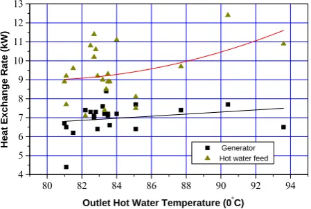
Figure 5 shows the effect of the inlet hot water temperature on the rate of heat transfer in the generator and hot water feed. Comparison of the simulation results show that the rate of heat transfer in the generator varies linearly, whereas in hot water feed, particularly at high temperatures and due to the effect of heat and electrical losses, variation of in the rate of heat transfer is non-linear. Figure 6 shows the effect of the generator's inlet hot water temperature on the outlet temperatures. As depicted from Figure 5, prediction of results implies a linear variation of the generator outlet temperature. A careful examination of Figures 5-8 reveals that the performance characteristics of the system in term of control variables could be approximated by a polynomial function of the order 2, as follows:

2 CX BX A

Y= + + (14)

Where, Y represents a performance parameter and X is a control variable. The coefficients A, B and C are determined based on the correlation of the experimental data using least-squares method. They are given in Table 5 for various operating conditions of the system.

6.2. Transient Mode

To investigate the system

TABLE 4. Simulation Results for System Performance (30th December 1999).

System Component/Parameters Description Unit Value Generator

Generator Temperature

Enthalpy of Solution Vapor at Outlet of Generator Temperature of Strong Solution in Inlet of Generator Absorbed Heat by Generator

Hot Water Flow Rate

°_C

kJ/kg

°_C

kJ/s kg/s

71.6 2621.2

52.9 6.23 0.45 Condenser

Condenser Temperature

Enthalpy of Saturated Liquid at Condenser Temperature Cooling Water Flow Rate

Heat Rejected

°_C

kJ/kg kg/s kJ/s

30.5 127.6 0.583 5.19 Evaporator

Evaporator Temperature

Enthalpy of Vapor at Evaporator Temperature Refrigerant Flow Rate

Cooling Capacity Air Flow Rate

°_C

kJ/kg kg/s kJ/s kg/s

-1.1 2499.1 0.0021 4.93 0.54 Absorber

Absorber Temperature

Heat Rejected by Cooling Water Concentration Ratio at Inlet Concentration Ratio at Outlet Flow Rate for Entering Solution Flow Rate for Exiting Solution Enthalpy of Entering Solution Enthalpy for Exiting Solution Heat Reject by Weak Solution

°_C

kJ/s - kg/s kg/s kJ/kg kJ/kg kJ/s

32.0 7.4 55.0 52.8 0.051 0.053 79.3 61.5 6.0 Heat Exchanger

Enthalpy of Entering Weak Solution Enthalpy of Exit Strong Solution

Temperature of Entering Strong Solution Effectiveness

Heat Absorbed by Solution

kJ/kg kJ/kg

°_C

- kJ/s

55.0 0.053

Figure 3. Time-thermal capacity and heat exchange history in various system components.

Figure 4. Time-temperature history of refrigerant and

LiBr-water solution at system components.

80 82 84 86 88 90 92 94

4 5 6 7 8 9 10 11 12 13 Generator Hot water feed

He at ex ch ang e rat e (Kw)

Inlet hot water temperature (oC)

Figure 5. The effect of inlet hot water temperature on heat

exchange rate in generator and hot water feed.

80 82 84 86 88 90 92 94

76 78 80 82 84 86 88 90 Out let hot wa ter t e mperat ure (o C)

Inlet hot water temperature (oC)

Figure 6. Variation of hot outlet water temperature vs. the inlet hot water temperature.

19 20 21 22 23 24 25

5 10 15 20 25 30

Chill water temperature

C h illed w a te r t e mp er at ure (o C)

Inlet cooling water temperature (oC₎

0 2 4 6 8 10 12 14 16 18 20 Cool ing l oad (Kw ) Cooling rate

Figure 7. Variation of chill water temperature and cooling rate

vs. inlet cooling water temperature.

5.0 5.5 6.0 6.5

0.50 0.55 0.60 0.65 0.70 0.75 0.80 0.85 COP CO P

Cooling rate (Kw)

10 100 Inl e t co ol in g w a te r temp eratu re (o C )

Inlet cooling water temperature

Figure 8. Variation of COP and inlet cooling water temperature vs. cooling capacity.

Cooling Rate (kW)

Heat Exchange Ra te (kW) Outlet Hot Wate r Temperature (0 ° C) In le t C ool ing Wate r Tempe ratur e (0 ° C)

Inlet Cooling Water Temperature (0°C)

C

ool

ing Load

(kW

)

Outlet Hot Water Temperature (0°

C) Chilled Wate r Tem p erature (0 °C)

Inlet Hot Water Temperature (0°C)

TABLE 5. Generalized Equation Coefficients-Performance Characteristics (Y) vs. Control Variable (X).

Y A B C X Ref.

Chilled Water Outlet Temp. (°_C)

Cooling Capacity (kW) Performance Coefficient (%) Inlet Cooling Water Temp. (°_C)

29.184 3.387 0.948 9.012

-1.290 0.693 -0.048 2.1297

0.048 -0.012

0.003 0

Inlet Cooling Temp. (°_C)

Inlet Cooling Temp. (°_C)

Cooling Load (kW) Cooling Load (kW)

Figure 8 Figure 8 Figure 9 Figure 9

0 10 20 30 40 50

e-3

e-2

e-1

e0

Generator Hot water feed Evaporator

D

imensionl

ess t

e

mp

er

at

ure

Time (min.)

Figure 9.Time-temperature history in various system components at transient mode.

ss , ev T o , ev T

ss , ev T ev T ev

θ

ss , hw T o , hw T

ss , hw T hw T hw

θ

ss , g T o , g T

ss , g T g T g

θ

− − =

− − =

− − =

(15)

Using Equation 15 and the data obtained from operating the system at transient mode (Table 2),

θg, θhw and θev can be calculated. The steady state

temperature Tg,ss, Thw,ss and Tev,ss are estimated

using the procedure discussed in Section 6.1 and using the data obtained by operating the system at

steady slate mode (Table 3). The results are plotted in Figure 9 on a logarithmic scale. A careful examination of the plots in Figure 9 reveals that the thermodynamic behavior of the generator and evaporator could be approximated by a straight line. On the other hand Equation 1 could be used to estimate the behavior of these components in the transient mode. The time-constant start up (τH in

Equation 1) can be estimated from Figure 9 to be 24 min. and 7.1 min. for the generator and evaporator, respectively.

Based on the above procedure a number of experiments have been carried out on the absorption cooling system in the transient mode (during 16th

November-30th _{December 1998). By analyzing the}

time-constant start up has been found in range of 18.8-33.3 minutes for generator and 2.8-150.0 minutes for evaporator, respectively. It should be emphasized that because of the relatively low heat exchange between the refrigerant and the air flow, over the surface of the evaporator, therefore, the time-constant start up for the evaporator is rather greater than that for the generator.

7. CONCLUSIONS

A computer simulation model for prediction of a LiBr absorption cooling system has been proposed. It is a component-oriented model and is capable of estimating the behavior of individual components and overall performance of the closed-cycle absorbent cooling system. It is also capable of making a sensitivity analysis in terms of some control variables.

The approach taken in the simulation was to describe the system in terms of components, design parameters and other required input that was recognized by the code. Thus it selects design parameters and carries out individual components analysis, system performance and makes a sensitivity analysis. A number of experiments on a 10 kW absorbent cooling system installed at MERC site have been carried out to validate the proposed model. The simulation results show that the performance characteristics of the system in terms of control variables can be estimated by generalized equations in the operation conditions for the system. Further investigation was carried out to estimate the system behavior at transient mode. The results show that the transient behavior of generator and evaporator can be estimated by an empirical function with a time-constant start up 18.8-33.3 min for generator and 2.8-150 min for evaporator, respectively, at common ranges of operating conditions for the system.

8. ACKNOWLEDGEMENTS

This work has been sponsored by the MERC, (Materials and Energy Research Center) under the contract No. 527904.

9. NOMENCLATURE

A Surface Area, m2

Cp Specific Heat Capacity, kJ/kg.K

h Enthalpy, kJ/kg

mo _{Mass Flow Rate, kg/s}

Q Absorbed or Rejected Heat Transfer Rate, kW

t Temperature, °_C

T Temperature, K

U Overall Heat Transfer Coefficient, kJ/m2_.K

Vo _{Discharge Flow Rate, m}3_/s

x Concentration Ratio (%)

Subscripts

ab Absorber c Condenser

cw Cooling Water

e Evaporator g Generator

hw Hot Water

hx Heat Exchanger

loss Heat Losses

min Minimum

o Initial Conditions

r Refrigerant

ss Steady State Conditions v.e Evaporative

Greek

ρ Density, kg/m3

θ Dimensionless Temperature

τ Time, s

τH Response Time Constant, s

10. APPENDEX

For any system operating conditions, x, the concentration ratio of salt in the solution in the range of 50 ≤ x ≤ 70 can be calculated by the following expression:

s 0.214t 37.5

s 1.107t 20

sol t 50 x

+ − ⎟ ⎠ ⎞ ⎜

⎝

⎛ ₋

+

TABLE 6. Coefficients of Equation 16 [10].

A0 = -2024.33 B0 = 18.2829 C0 = -3.7008214 E-2

A1 = 163.309 B1 = -1.1691757 C1 = 2.887666 E-3

A2 = -4.88161 B2 = 3.248041 E-2 C2 = -8.1313015 E-5

A3 = 6.302948 E-2 B3 = -4.034184 E-4 C3 = 9.9116628 E-7

A4 = -2.913705 E-5 B4 = 1.8520569 E-6 C4 = -4.4441207 E-9

Where tsol is the solution temperature and ts is the

saturation temperature at the solution pressure. The enthalpy of solution can be determined from following expression [10]:

n x 4

0Cn

n x 4

0Bn

4

0 n x n A

h=∑ +∑ +∑ (17)

Where h is the enthalpy in kJ/kg and t is the temperature in °_{C. Equation 16 is valid for the}

range of:

50 ≤ x ≤ 70 and 15°_{C ≤ x ≤ 165}°_C.

The coefficients of An, Bn, Cn are given by Table 6.

11. REFERENCES

1. Grassie, S. L. and Sheridan, N. R., “Modeling of a Solar-Operated Absorption Air Conditioner System with Refrigerant Storage”, Solar Energy, Vol. 19, (1977), 691-700.

2. Ameel, T. A., Gee, K. G. and Wood, B. D., “Performance Predilections of Alternative, Low Cost Absorbents for Open Cycle Absorption Solar Cooling”,

Solar Energy, Vol. 54, No. 2, (1995), 65-73.

3. Wardono, B. and Nelson, R. M., “Simulation of a Double-Effect LiBr/H2O Absorption for Cooling

System”, ASHRAE Transaction, Vol. 38, No. 10, (1996), 32-38.

4. Eicker, U., Jakob, U., Schneider, D., Bauer, U., Spindler, K., Bremded, T., Negro, E. and Diepolder, W., “Design of a Solar Driven Cooling Unit Based on the Diffusion Absorption Principle”, Technical Report for the European Commission, Fachhochule Stuttgart-Hochschule fur Technik, Contract No. JOE-CT98-7045, Germany, (2001).

5. Vliet, G. C., Lawson, M. B. and Lithgow, R. A., “Water-Lithium Bromide Double Effect Absorption Cooling Cycle Analysis”, ASHRAE Transactions, Vol. 88, No. 1, (1982), 811-823.

6. Grossman, G. and Childs, K. W., “Computer Simulation of a Lithium Bromide-Water Absorption Heat Pump for Temperature Boosting”, ASHRAE Transactions, Vol. 88, No. 1, (1982), 811-823.

7. Grossman, G., Gommed, K. and Gadoth, D., “A Computer Model for Simulation of Absorption Systems in Flexible and Modular Form”, ASHRAE

Transactions, Vol. 93, No. 2, (1987), 2389-2428.

Cooling”, Solar Energy, Vol. 49, No. 6, (1992), 515-534.

9. Duffie, J. A. and Beckman, W. A., “Solar Engineering of Thermal Processes”, John Willey and Sons, New

York, U.S.A., (1992).