A HOLISTIC APPROACH BASED ON MCDM FOR SOLVING
LOCATION PROBLEMS
A. Kaboli, M. B. Aryanezhad* and K. Shahanaghi
Department of Industrial Engineering, Iran University of Science and Technology P.O. Box 16844, Tehran, Iran
[email protected] - [email protected] - [email protected]
R. Tavakkoli-Moghaddam
Engineering Optimization Research Group, Department of Industrial Engineering Faculty of Engineering, University of Tehran
P.O. Box 11365/4563, Tehran, Iran [email protected]
*Corresponding Author
(Received: December 25, 2006 – Accepted in Revised Form: September 13, 2007)
Abstract Location decision is an integral part of organizational strategies involving many factors that may be conflicting in nature. This paper presents a holistic approach of the multi-criteria decision making (MCDM) methodology to select the optimal location(s), which fits best for both investors and managers. A case study is also provided to illustrate the application of the proposed holistic approach. Finally, a comparison with the previous work is made and the informational efficacy of the proposed model is also discussed.
Keywords Location Selection, Multi-Criteria Decision Making (MCDM), Fuzzy AHP
ﻩﺪﻴﻜﭼ
ﯼﺭﺎﻴﺴـﺑﻞـﻣﺍﻮﻋﻞﻣﺎﺷﻭﺖﺳﺍﻲﻧﺎﻣﺯﺎﺳﯼﮋﺗﺍﺮﺘﺳﺍﮏﻔﻨﻳﻻﺀﺰﺟﺕﻼﻴﻬﺴﺗﻥﺎﮑﻣﺩﺭﻮﻣﺭﺩﻢﻴﻤﺼﺗﺫﺎﺨﺗﺍ
ﺘﻴﻫﺎﻣﺖﺳﺍﻦﮑﻤﻣﻪﮐﺖﺳﺍ
ﺎ
"
ﺪﻨﺷﺎﺑﺽﺭﺎﻌﺗﺭﺩ
.
ﻱﺍﺮـﺑﻩﺭﺎـﻴﻌﻣﺪﻨﭼﯼﺮﻴﮔﻢﻴﻤﺼﺗﻊﻣﺎﺟﺩﺮﮑﻳﻭﺭﻚﻳﻪﻟﺎﻘﻣﻦﻳﺍﺭﺩ
ﺩﺎﻬﻨﺸﻴﭘﻪﻨﻴﻬﺑﻥﺎﮑﻣﺏﺎﺨﺘﻧﺍ ﻲﻣ
ﻪﻳﺎﻣﺮﺳﻭﻥﺍﺮﻳﺪﻣﺕﻼﻳﺎﻤﺗﺎﺑﻪﮐﺩﺩﺮﮔ
ﺖـﺳﺍﻖﺒﻄﻨﻣﻥﺍﺭﺍﺰﮔ
. ﺩﺮـﮑﻳﻭﺭﻦـﻳﺍﺩﺮﺑﺭﺎـﮐ
ﺖﺳﺍﻩﺪﺷﻩﺩﺍﺩﺡﺮﺷﯼﺩﺭﻮﻣﻪﻌﻟﺎﻄﻣﮏﻳﺎﺑﻊﻣﺎﺟ
.
ﺎﺑﻪﺴﻳﺎﻘﻣ،ﻥﺎﻳﺎﭘﺭﺩ
ﺵﻭﺭﯼﺪﻨﻣﺩﻮﺳﻭﻩﺪﺷﻡﺎﺠﻧﺍﻲﻠﺒﻗﯼﺎﻫﺭﺎﮐ
ﺮﮔﺭﺍﺮﻗﺚﺤﺑﺩﺭﻮﻣﻩﺪﺷﻪﻳﺍﺭﺍ ﺖﺳﺍﻪﺘﻓ
.
1. INTRODUCTION
Over the years, one of the most prominent corporate growth strategies has been the expansion into global markets [1]. Global expansion offers access to new markets and opportunities to utilize economies of scale. In today's global economy, characterized by a dynamic and volatile environment, many researchers stress the significance of international location factors [2]. Location decisions are made in public and private sectors. For example, governments need to determine the locations for emergency bases highway patrol vehicles, fire bases, ambulances, television antennas, and exploratory oil wells. In all cases, poor locations can increase the likelihood of property damage and cost life. In private sectors,
engineering, urban planning, and related fields [3,4]. Summing up, the success or failure of both private and public sector facilities depends in part on the facilities locations.
Location theory was first introduced by Weber [5], who considered the problem of locating a single warehouse in order to minimize the total travel distance between the warehouse and a set of spatially distributed costumers. In fact, he proposed a material index for selecting the location in which if this index is grater than one, the warehouse should be installed in the vicinity of the source of raw material; or otherwise, it should be close to the market. Isard [6] reconsidered this work with the study of the industrial location, land use, and the related problems. Hotelling [7] introduced another problem of locating two competing vendors along a straight line. Smithies and Stevens [8,9] extended the Hotelling's problem later. Hakimi [10] considered a general problem to locate one or more facilities on a network by minimizing the sum of the distances and the maximum distance between facilities and points on a network. Considerable research and theoretical interest in the location problem have been carried out after this seminal paper.
Brown and Gibson [11] and Buffa and Sarin [12] proposed a facility location model for a multi-dimensional location problem based on critical factors, objective factors, and subjective factors. Fortenberry and Mitra [13] presented a model for the location-allocation problems considering both qualitative and quantitative factors. Kahne [14] considered 29 attributes and used a weighting model to determine the relative importance with uncertainty in attributes. Charnetski [15] considered the case of selecting one of the three proposed sites for a modern air terminal with a large number of attributes.
A few studies on power plant site evaluation carried out after the Keeney and Nair [16] have been studied on the identification and recommendation of potential new sites for a nuclear power facility. Kirkwood [17] discussed a multi-disciplinary study conducted to select a site for a nuclear power facility. Linares and Romrero [18] proposed a methodology that combined several multi-criteria methods to address electricity planning problems. The analytic hierarchy process (AHP) is an analytical approach used to solve complex
problems. Some researchers used the AHP as a stand-alone methodology to make location decisions [19,20]. The AHP enables the decision maker to structure a complex problem in the form of a simple hierarchy and to evaluate a large number of quantitative and qualitative factors in a systematic manner with conflicting multiple criteria [21]. Other MCDM methods for the location selection are used such as Liang and Wang [22] who proposed an algorithm for a site selection based on the concepts of the fuzzy set theory. Bahattacharya et al. [23] proposed a holistic MCDM model for the facility location selection. Yong [24] proposed a fuzzy TOPSIS approach to select the best facility location under linguistic environment. Brown and Gibson [11] and Buffa and Sarin [12] proposed a model that classifies the objective and subjective factors important to the specific location problem being addressed as: critical, objective, and subjective. Bahattacharya et al. [23] eliminated critical factors from their model and proposed a holistic method for the facility location selection based on Brown and Gibson [11] and Buffa and Sarin [12]. The benefit of extending crisp theory and analysis methods to fuzzy techniques is the strength in solving real-world problems, which inevitably entail some degree of imprecision and noise in the variables and parameters measured and processed for the application [22]. Kaboli et al. [25,26] used this combined approach to present a mathematical model for the site selection.
This paper proposes a multi-criteria decision making (MCDM) methodology that is suitable for a location problem under conflicting in nature criteria environment. The main goal of this paper is to provide investors and managers with a more effective and efficient model for location selection decisions. The purpose of this paper is also to demonstrate how better location decisions can be made by the application of the fuzzy AHP (FAHP). Furthermore, a multi-attribute location with triangular fuzzy numbers model is discussed to give a clear indication about the location selection problem in real-world situations.
General goal Select the best location (s)
Work culture Recreational
facility
Transportation availability
Housing facility
Climatic condition
Criteria
Locations L
2
L1 L3 L4 L5
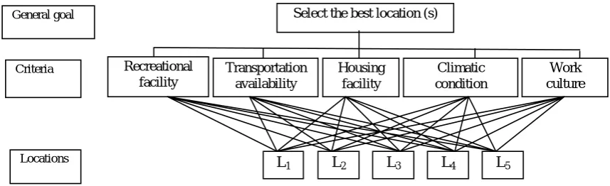
Figure 1. Hierarchy process for the location selection. effectiveness of the proposed model in the facility
location problem. Finally, this paper concludes with a summary and applications to the future work.
2. PROPOSED MATHEMATICAL MODEL
The following notations were used in the state of equations and relations:
α Objective factor decision weight.
FOFM Fuzzy objective factors measures.
FSFM Fuzzy subjective factor measures.
FOFC Fuzzy objective factor components.
FLSI Fuzzy location selection index.
FOFMi are determined by Equation 1:
(
)
(
)
11
i i i
FOFM =⎡⎣ FOFC ×
∑
OFC − ⎤⎦− (1)FSFMi values are nothing but the global priority
for each location. FSFMi may be found by
multiplying each of the decision matrix PV values to each of the PV values of the location for each factor. The product is then summed up for each alternative [23]. The locations are ranked based on
FLSIi index as shown in Equation 2.
(
) (
1)
i i i
FLSI =⎡⎣α×FSFM + −α ×FOFM ⎤⎦ (2)
The choice of α is an important issue. In order to make a better comparison and benchmark of the proposed approach, the α value is set to 0.36 as given in [23].
3. PROPOSED METHODOLOGY
3.1. Proposed Algorithm
Weextend the work proposed by Bhattacharya et al. [23], in which they used their proposed model for the facility location selection. However, we consider the fuzzy values for criteria. The general goal, criteria, and location alternatives are presented in Figure 1 illustrating the hierarchy for the location selection problem. The first level of the hierarchy shows that the general goal is to select the best location. At the second level, the five criteria subjective factors stated by Kulkarni et al. [25] are: recreational facility, transportation availability, housing facility, climatic condition, and work culture. At the third level, five location alternatives are chosen for selection. All of these levels will contribute to the achievement of the general goal.3.2. Fuzzy Analytic Hierarchy Process
(FAHP)
The concept of the analytic hierarchy process (AHP) was first developed by Saaty [28,29]. This method is a robust, flexible multi-criteria decision analysis tool. The AHP methodology is a decision-support procedure for dealing with complex, unstructured, and multi-criteria decisions [30]. Three basic steps of this methodology are as follows:• Describing a complex decision making problem as a hierarchy.
• Using pair-wise comparison techniques in estimating the relative weights of various elements on each level of the hierarchy. • Integrating the weights to develop an overall
l m u M 0.0
1.0
μ
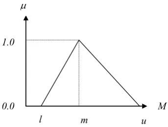
Figure 2. A triangular fuzzy number. The concept of the fuzzy set theory was first
introduced by Zadeh [31]. It has been used as a modeling tool for complex systems that are difficult to define precisely or with certainty, but can be operated and controlled by humans. There are many fuzzy AHP methods proposed by a number of researchers. The earliest research in the fuzzy AHP was appeared in Van Laarhoven and Pedrycz [32]. Chang [33] introduced a new approach to fuzzy AHP and proposes triangular fuzzy numbers for pair-wise comparison scale of fuzzy AHP in his model. Other models and applications of fuzzy AHP for evaluating weapon systems, technology selection algorithm, and integrated approach for the design of flexible manufacturing system (FMS) are proposed [34-36]. Kuo et al. [37] developed a decision support system to find a new convenience store locations. Kahraman et al. [38] applied an analytical tool to select the best catering firm providing the most customer satisfaction.
By embedding the AHP method into fuzzy sets, another application area of the fuzzy logic is revealed. Decision markers usually find that it is more confident to give interval judgments than fixed value judgment. This is because they are usually unable to be explicit about their preferences due to the fuzzy nature of the comparison process [38]. Due to relatively easier steps of Chang’s extension than the other fuzzy AHP approaches and similarity to the crisp AHP, we use this approach in our proposed model by applying the steps of extent analysis approach introduced by Zhu et al. [39]. To state the fuzzy AHP approach, let us have an introduction from the triangular fuzzy numbers at first. A major contribution of the fuzzy set theory is its capability of representing vague data. This theory also allows mathematical operations and programming to apply to the fuzzy domain. A fuzzy set is a class of objects with a continuum of grades of membership. Such a set is characterized by a membership (characteristic) function, which assigns to each object a grade of membership ranging between zero and one.
A triangular fuzzy number is shown in Figure 2. A triangular fuzzy number is denoted simply as (l|m,m|u) or (l,m,u). The parameters l, m, and u denote the smallest possible value, the most promising value, and the largest possible value, respectively, describing a fuzzy event. Now, let
{
1, 2,..., n}
X = x x x be an object set, and
{
1, 2,..., m}
U = u u u be a goal set according to the method of Chang's [40] extent analysis, each object is taken and extent analysis for each goal, gi,
is performed, respectively. Therefore, m extent analysis value for each object can be obtained, with the following signs:
1
,
2,...,
m;
1,2,...,
gi gi giL L
L i
=
n
(3)where, all the L ( j = 1,2,...,m)gij are triangular fuzzy numbers [39]. The steps of Chang's extent analysis can be given below:
Step 1. The value of fuzzy synthetic extent with respect to the ith object is defined as follows:
1
1 1 1
m n m
j j
i gi gi
j i j
S L L
−
= = =
⎡ ⎤
= ⊗ ⎢ ⎥
⎣ ⎦
∑
∑∑
(4)To elaborate
∑
mj i= Lgij , perform the fuzzy addition operation of m extent analysis values for a particular matrix such that:1 1 1
, ,
m m m m
j
gi j j j
j i j j j
L l m u
= = = =
⎛ ⎞
= ⎜ ⎟
⎝ ⎠
∑
∑ ∑ ∑
(5)and to obtain
1 1 1 n m j gi j j L − = = ⎡ ⎤ ⎢ ⎥
l2
L2 L1
1
(
2 1)
V L ≥L
m2 l1 d u2 m1 u1
Figure 3. The intersection between L1 and L2. addition operation of L ; Jgij ( =1, 2,...,m) values
such that:
1 1 1 1 1
, ,
n m m m m
j
gi i i i
j j i i i
L l m u
= = = = =
⎛ ⎞
= ⎜ ⎟
⎝ ⎠
∑∑
∑ ∑ ∑
(6)and then compute the inverse of the vector in Equation 6 such that
1
1 1
1 1 1
1 1 1
, ,
n m j
gi n n n
j j
i i i
i i i
L
u m l
− = = = = = ⎛ ⎛ ⎞ ⎛ ⎞⎞ ⎜ ⎜ ⎟ ⎜ ⎟⎟ ⎡ ⎤ ⎜ ⎟ ⎜ ⎟ ⎜ ⎟ = ⎢ ⎥ ⎜ ⎟ ⎜ ⎟ ⎜ ⎟ ⎣ ⎦ ⎜ ⎟ ⎜ ⎟ ⎜ ⎝ ⎠ ⎝ ⎠⎟ ⎝ ⎠
∑∑
∑
∑
∑
(7)Step 2.
SinceL
1 andL
2 are convex fuzzy numbers, the degree of possibility of(
)
(
)
2 2, 2, 2 1 1, 1, 1
L = l m u ≥L = l m u stated as
follows:
(
)
(
) (
)
2 1 2 2 1 1 22 2 1 1
1
0 1
m m
l u
V L L
l u
Otherwise.
m u m l
≥ ⎧ ⎪ ⎪⎪ ≥ ≥ = ⎨ ⎪ − ⎪ − − − ⎪⎩ (8)
where, d is the ordinate of the highest intersection point
D
betweenμ
( )
L1 andμ
( )
L2 , which is depicted in Figure 3. To compare M1and M2, both values of V L(
1≥L2)
and V L(
2≥L1)
are needed.Step 3.
The degree possibility for a convex fuzzy number to be greater thank
convex fuzzy numbers L ii(
=1, 2,...,k)
can be defined by the following equation.( 1, 2, ..., k)
[
( 1) (, 2),...,( k)]
V L≥L L L =V L ≥L L ≥L L ≥L
(
)
=Min 1, 2, ..., .V M ≥Mi
;
i = k(9)
Assume that '
( )
(
)
min
i i k
d A = V S ≥S for
1, 2, ..., ; .
k = n k ≠i Then, the weight vector is given below.
( ) ( )
( )
(
)
' ' ' '
1 , 2 , ...,
T n
W = d A d A d A (10)
where, A ii
(
=1, 2, ...,n)
aren
elements.Step 4.
Via normalization, the normalized weight vectors are as follows:( ) ( )
( )
(
1 , 2 , ...,)
T n
W = d A d A d A (11)
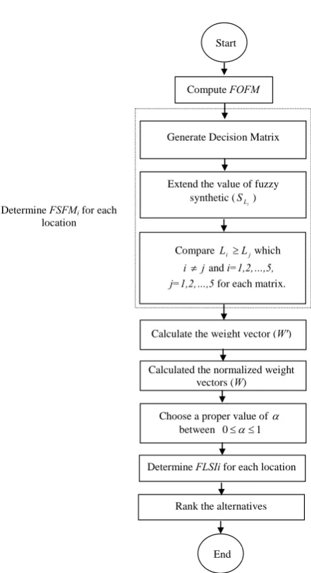
where, W is a non-fuzzy number [25,26,38]. The priority weights of important attributes by an eigenvector method for each pair-wise comparison, matrices are calculated and by the usage of FAHP, global priorities of attributes are found as the fuzzy subjective factor measures (FSFM) in Equation 5. Then the pair-wise comparison matrices for five different factors (Table 3 to Table 8) are constructed based on Satty’s nine-point scale. The fuzzy objective factors measures (FOFM) and fuzzy objective factor components (FOFC) are calculated separately by the use of cost factors given in Table 1. Furthermore, to summarize the stated solving method, the proposed approach is illustrated in Figure 4 step by step.
To rank and choose the best location from the pool of alternatives, first the fuzzy objective factors measures (FOFMi) for each location must
be computed. Second, FSFMi for each location
TABLE 1. Cost Factor Components and Their Units.
Cost of Components Units Cost of Land (*103) US. $ Cost of Raw Material US. $/ Kg
Cost of Energy US. $/ Unit of Electric Energy
Cost of Transportation US. $/ Item Cost of Labor US. $/ Labor-Day
Determine FSFMi for each
location
Rank the alternatives
End Compute FOFM
Start
Extend the value of fuzzy synthetic (
i
L
S )
Compare Li ≥Ljwhich
i≠jand i=1,2,…,5, j=1,2,…,5 for each matrix. Generate Decision Matrix
Calculate the weight vector (W')
Determine FLSIi for each location Calculated the normalized weight
vectors (W)
Choose a proper value of α between 0≤ ≤α 1
Figure 4. The proposed approach for facility location selection.
obtain the normalized weight vector (W). Then, with a proper value of α, based on the decision maker's preference, fuzzy location selection index (FLSIi) is determined for each location.
4. A CASE STUDY
To benchmark the proposed MCDM approach, a case study is illustrated in this section. The problem considers tangible factors such as: cost of land, cost of transportation, cost of energy, cost of raw material, and cost of land as cost factor components as tabulated in Table 1. In addition, Kulkarni et al. [27] stated intangible factors such as: work culture, climatic condition, housing facility, transportation availability, and recreational facility. One may consider other important attributes in a facility location selection like Badri [19], Min [20], and Yang [21]. Assume that a company is trying to select a location to build a new facility from five alternatives. The triangular fuzzy numbers are presented in Table 2.
5. COMPUTATIONAL RESULTS
The proposed methodology is coded and solved as a computer program in C language that enables the user to select the most suitable site among available selection. Tables 3 to 8 show the comparison matrix factors for each of the factors.
Table 9 consolidates the results of the earlier tables in arriving at the composite weight, FSFM, of each of the alternatives. Table 10 shows the final ranking based on the proposed methodology and the comparison with the previous work.
TABLE 2. Triangular Fuzzy Numbers of Cost Factor Components.
Facility Location
Cost of Components L1 L2 L3 L4 L5
Cost of Land (*103) (71,72,74) (134,135,137) (49,50,52) (64,65,67) (99,100,102) Cost of Raw Material (24,25,27) (6,17,19) (22,35, 25) (19,20,22) (14,15,17)
Cost of Energy (0.5,1.5,3.5) (0,0.5,2.5) (0,0.9,2.9) (0,1,3) (0.3,1.3,3.3) Cost of Transportation (2,3,5) (0,1,3) (3,4,6) (1,2,4) (1.5,2.5,4.5)
Cost of Labor (66,67,69) (59,60,62) (69,70,72) (55,56,58) (57,58,60)
TABLE 3. Pair-Wise Comparison Matrix for F1.
F1 L1 L2 L3 L4 L5
L1 (1,1,1) (4,5,6) (1,2,3) (7,8,9) (3,4,5)
L2 (1/6,1/5,1/4) (1,1,1) (1/6,1/5,1/4) (1,2,3) (1/4,1/3,1/2)
L3 (3,4,5) (1,2,3) (1,1,1) (4,5,6) (6,7,8)
L4 (1/4,1/3,1/2) (4,5,6) (1/6,1/5,1/4) (1,1,1) (2,3,4) L5 (1/5,1/4,1/3) (5,6,7) (1/8,1/7,1/6) (1/4,1/3,1/2) (1,1,1)
TABLE 4. Pair-Wise Comparison Matrix for F2.
F2 L1 L2 L3 L4 L5
L1 (1,1,1) (1/3,1/2,1) (1/5,1/4,1/3) (2,3,4) (3,4,5)
L2 (1,2,3) (1,1,1) (1/3,1/2,1) (4,5,6) (5,6,7)
L3 (3,4,5) (1,2,3) (1,1,1) (4,5,6) (6,7,8)
L4 (1/4,1/3,1/2) (4,5,6) (1/6,1/5,1/4) (1,1,1) (2,3,4)
L5 (1/5,1/4,1/3) (5, 6, 7) (1/8,1/7,1/6) (1/4,1/3,1/2) (1,1,1)
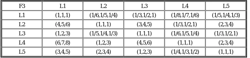
TABLE 5. Pair-Wise Comparison Matrix for F3.
F3 L1 L2 L3 L4 L5 L1 (1,1,1) (1/6,1/5,1/4) (1/3,1/2,1) (1/8,1/7,1/6) (1/5,1/4,1/3)
L2 (4,5,6) (1,1,1) (3,4,5) (1/3,1/2,1) (2,3,4)
L3 (1,2,3) (1/5,1/4,1/3) (1,1,1) (1/6,1/5,1/4) (1/3,1/2,1) L4 (6,7,8) (1,2,3) (4,5,6) (1,1,1) (2,3,4)
TABLE 6. Pair-Wise Comparison Matrix for F4.
F4 L1 L2 L3 L4 L5
L1 (1,1,1) (1/3,1/2,1) (4,5,6) (2,3,4) (2,3,4)
L2 (1,2,3) (1,1,1) (5,6,7) (4,5,6) (4,5,6)
L3 (1/6,1/5,1/4) (1/7,1/6,1/5) (1,1,1) (1/3,1/2,1) (1/4,1/3,1/2) L4 (1/4,1/3,1/2) (1/5,1/4,1/3) (3,4,5) (1,1,1) (1,2,3) L5 (1/4,1/3,1/2) (1/6,1/5,1/4) (2,3,4) (1/3,1/2,1) (1,1,1)
TABLE 7. Pair-Wise Comparison Matrix for F5.
F5 L1 L2 L3 L4 L5
L1 (1,1,1) (1/3,1/2,1) (3,4,5) (5,6,7) (4,5,6)
L2 (1,2,3) (1,1,1) (2,3,4) (2,3,4) (1,2,3)
L3 (1/5,1/4,1/3) (1/4,1/3,1/2) (1,1,1) (6,7,8) (1/5,1/4,1/3) L4 (1/7,1/6,1/5) (1/4,1/3,1/2) (1/8,1/7,1/6) (1,1,1) (1/4,1/3,1/2)
L5 (1/6,1/5,1/4) (1/3,1/2,1) (3,4,5) (2,3,4) (1,1,1)
TABLE 8. Comparison Matrix.
F1 F2 F3 F4 F5
F1 (1,1,1) (5,6,7) (4,5,6) (2,3,4) (6,7,8)
F2 (1/7,1/6,1/5) (1,1,1) (1/8,1/7,1/6) (1/8,1/7,1/6) (1,2,3) F3 (1/6,1/5,1/4) (6,7,8) (1,1,1) (1/4,1/3,1/2) (2,3,4)
F4 (1/4,1/3,1/2) (6,7,8) (2,3,4) (1,1,1) (4,5,6)
F5 (1/8,1/7,1/6) (1/3,1/2,1) (1/4,1/3,1/2) (1/6,1/5,1/4) (1,1,1)
TABLE 9. Matrix for Computing FSFM.
F1 F2 F3 F4 F5 0.431 0 0 0.25 0.25
FSFM
L1 0.635 0 0 0.286 0.459 0.640
L2 0 0.333 0.333 0.429 0.286 0.179
L3 0.375 0.5 0 0 0.111 0.189
L4 0 0.111 0.61 0 0 0
TABLE 10. Rank of the Alternatives Based on the Proposed Model.
Rank No. Proposed Approach
FLSIi Location
Previous Work [23]
LSIi Location
1 0.298 L1 0.259 L3
2 0.259 L3 0.251 L1
3 0.147 L4 0.194 L4
4 0.135 L2 0.153 L2
5 0.126 L5 0.141 L5
0.0 0.1 0.2 0.3 0.4 0.5 0.6 0.7
0 0.1 0.2 0.3 0.4 0.5 0.6 0.7 0.8 0.9 1
FLS
I i
L1
L2
L3
L4
L5
Figure 5. Sensitivity analysis. 0.36, where 0≤ ≤α 1 and for α = 1, FLSI = FSFM
which means that selection is dependent on fuzzy subjective factor measure values found from fuzzy AHP, and FSFM values dominate over FOFM values. Also, for α = 0 the cost factors have priority over the intangible factors.
The comparison of the proposed approach with the previous work shows the more accuracy of this new method. Location L1 has more priority than L3 and the other locations with lower weights than the pervious work are sorted as before. Also the ability to make more desired location's a priority and lower undesired location's priority can be depicted from this comparison. The sensitivity analysis is next shown to verify the practicality and efficacy of the associated results of the proposed approach.
Due to the dynamic nature of the decision environment in real life situations, it is essential to equip the proposed model with the capability to
distinguish changes in the facility selection process. As mentioned above, the related equation for each of the five alternatives of site for plant location is given bellow:
(
) (
1)
i i i
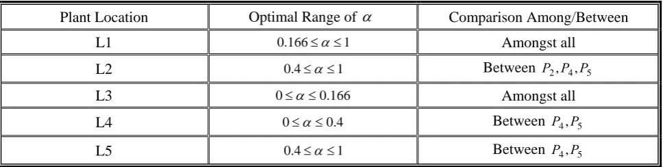
FLSI =⎡⎣α×FSFM + −α ×FOFM ⎤⎦ (12) As the value of the objective factor decision weight lies between 0 and 1, the lines are drawn for each location for evaluation ranging between 0 and 1 as shown in Figure 5.
TABLE 11. Analysis of Figure 5.
Plant Location Optimal Range of α Comparison Among/Between
L1 0.166≤ ≤α 1 Amongst all
L2 0.4≤ ≤α 1 Between P P P2, 4, 5
L3 0≤ ≤α 0.166 Amongst all
L4 0≤ ≤α 0.4 Between P P4, 5
L5 0.4≤ ≤α 1 Between P P4, 5
moving to lower than 0.5 will result in dominancy of cost factor components. So, the intangible factors will get less priority. In summation, it is essential to justify a proper value forα.
6. CONCLUSION
A facility location selection problem can be directed either toward an organization in search of a site to locate or relocate its facility to maximize the utilization of resources and minimize the overall cost. In this paper, a novel mathematical model for the site selection is proposed for a facility location problem. An MCDM methodology has been used for the organizations seeking a site for new facility, or a relocation of existing facilities. The solution procedure was illustrated through a case study. Any changes in the decision maker's preferences, α ratio and costs could affect the desirability of a specific location that was considered in this holistic model. As shown in this paper, Location L1 has more priority than L3 and the other locations with lower weights than the pervious work are sorted as before. Furthermore, the proposed approach has the ability to make more desired location's priority and lower undesired location's priority can be taken from this comparison. The result of the proposed model and comparison with previous work has shown the effectiveness and adaptability of our holistic model with the real-world problems. Future research can
be considered as a framework for making a decision under uncertainty, developing a decision model to help decision makers in large-scale location problems, and allocating demands to the related locations.
7. AKNOWLEDGEMENT
The authors would like to thank the anonymous reviewers for their helpful comments and suggestions, which greatly improved the presentation of this paper.
8. REFERENCES
1. Hoffman, J. and Schniederjans, M., “A two-stage model for structuring global facility site selection decisions”,
International Journal of Operations and Production Management, Vol. 14, No. 4, (1997), 79-96.
2. Badri, M. and Davis, D., “Decision support models for the location of decision support models for the location of firms in industrial sites”, International Journal of Operations and Production Management, Vol. 15, No. 1, (1995), 50-62.
3. Daskin, M. S., “Network and discrete location: Models, algorithms, and applications”, John Wiley and Sons, New York, (1995).
4. Derzner, Z., “Facility location: A survey of applications and methods”, Springer-Verlag Inc., New York, (1995). 5. Brandeau, M. L. and Chiu, S. S., “An overview of
representative problems in location research”,
Press, MIT, Cambridge, MA, (1956).
7. Hotelling, H., “Stability in competition”, Economic Journal, Vol. 39, (1929), 41-57.
8. Smithies, A., “Optimum location in spatial competition”,
Journal of Political Economy, Vol. 49, (1941), 432-492.
9. Stevens, B. H., “An application of game theory to a problem in location strategy”, Papers of Regional Science Association, Vol. 7, (1969), 85-111.
10. Hakimi, S. L., “Optimal locations of switching centers and the absolute centers and medians of a graph”,
Operations Research, Vol. 12, (1964), 450-459. 11. Brown, P. A. and Gibson, D. F., “A quantified model
for facility site selection: An application to a multi-facility location problem”, AIIE Transactions, Vol. 4, (1972), 1-10.
12. Buffa, E. S. and Sarin, R. K., “Modern production and operations management”, 8th edition, John Wiley and Sons, New York, (1987).
13. Fortenberry, J. C. and Mitra, A., “A multiple criteria approach to the location-allocation problem”, Computer and Industrial Engineering, Vol. 10, No. 1, (1986), 77-87.
14. Kahne, S., “A procedure for optimizing development decisions”, Automatica, Vol. 11, No. 3, (1975), 261-269.
15. Charnetski, J. R., “Multiple criteria decision making with partial information: A site selection problem”, Space Location-Regional Development, Pion, London, (1976), 51-62.
16. Keeny, R. L. and Nair, K., “Selecting nuclear power facility sites in the pacific northwest using decision analysis”, Conflicting Objectives in Decisions, New York, (1977), 298-322.
17. Kirkwood, C. W., “A case history of nuclear power facility site selection”, Journal of Operational Research Society, Vol. 33, (1982), 353-363.
18. Linares, P. and Romero, C., “A multiple criteria decision making approach for electricity planning in Spain: Economic versus environmental objectives”,
Journal of Operational Research Society, Vol. 51, (2000), 736-743.
19. Min, H., “Location planning of airport facilities using the analytic hierarchy process”, Logistics and Transportation Review, Vol. 30, 1, (1994), 79-94. 20. Yang. J., and Lee, H., “An AHP decision model for
facility location selection”, Facilities, Vol. 15, (1997), 241-254.
21. Badri, M. A., “Combining the Analytic Hierarchy Process and Goal Programming for Global Facility Location-Allocation Problem”, International Journal of Production Economics, Vol. 62, (1999), 237-248. 22. Liang, G. S. and Wang, M, J., “A fuzzy multi-criteria
decision making method for facility site location”,
International Journal of Production Research, Vol. 29, No. 11, (1999), 2313-2330.
23. Bhattacharya, A., Sarkar, B. and Mukherjee, S. K., “A new method for facility location selection: A holistic approach”, International Journal of Industrial Engineering: Theory, Applications, and Practice, Vol. 11, No. 4, (2004), 330-338.
24. Yong, D., “Facility location selection based on fuzzy TOSIS”, International Journal of Advanced Manufacturing Technology, Vol. 28, (2006), 839-844. 25. Kaboli, A., Aryanezhad, M. B. and Shahanaghi, K., “A
new method for location selection: A hybrid analysis”,
Proceedings of the Second International Conference on Modeling, Simulation and Applied Optimization, (ICMSAO), Abu Dhabi, United Arab Emirates, (March, 2007).
26. Kaboli, A., Aryanezhad, M. B., Shahanaghi, K. and Niroomand, I., “A mathematical method for location problem: A fuzzy-AHP approach”, Proceedings of the IEEE International Conference Systems, Man, and Cybernetics, Canada, (October, 2007).
27. Kulkarni, M., Nalgirkar, M. and Mital, A., “Quantifying subjective descriptors for the facility location problem”,
International Journal of Industrial Engineering: Theory, Applications, and Practice, Vol. 1, No. 2, (1994).
28. Saaty, T., “The analytic hierarchy process”, McGraw-Hill, New York, (1980).
29. Saaty, T., “How to make a decision: the analytic hierarchy process”, European Journal of Operational Research, Vol. 48, No. 1, (1990), 9-26.
30. Dasarathy, B. V., “SMART: Similarity measure anchored ranking- technique for the analysis of multidimensional data analysis”, IEEE Transactions on Systems, Man, and Cybernetics, SMC-6, Vol. 10, (1976), 708-711.
31. Zadeh, F., “The analytic hierarchy process: A survey of the method and its applications”, Interfaces, 16 (4), (1986), 96-108.
32. Van Laarhoven, P. J. M. and Pedrycz, W., “A fuzzy extension of Saaty’s priority theory”, Fuzzy Sets and Systems, Vol. 11, (1983), 229-241.
33. Chang, D.-Y., “Applications of the extent analysis method on fuzzy AHP”, European Journal of Operational Research, Vol. 95, (1996), 649-655. 34. Cheng, C.-H., Yang, K.-L. and Hwang, C.-L.,
“Evaluating attack helicopters by AHP based on linguistic variable weight”, European Journal of Operational Research, Vol. 116, 2, (1999), 423-435. 35. Chan, F. T. S., Chan, M. H. and Tang, N. K. H.,
“Evaluation methodologies for technology selection”,
Journal of Materials Processing Technology, Vol. 107, (2000), 330-337.
36. Chan, F. T. S., Jiang, B. and Tang, N. K. H., “The development of intelligent decision support tools to aid the design of flexible manufacturing systems”,
International Journal of Production Economics, Vol. 65, No. 1, (2000), 73-84.
37. Kuo, R. J., Chi, S. C. and Kao, S. S., “A decision support system for selecting convenience store location through integration of fuzzy AHP and artificial neural network”, Computers in Industry, Vol. 47, No. 2, (2002), 199-214.
39. Zhu, K.-J., Jing, Y. and Chang, D.-Y., “A discussion of extent analysis method and applications of fuzzy AHP”,
European Journal of Operational Research, Vol. 116,
(1999), 450-456.
40. Chang, D. Y. “Extent analysis and Synthetic Decision”,