Investigation of Fluid-structure Interaction by Explicit Central Finite Difference Methods

Please cite this article as: F. Khalighi, A. Ahmadi, A. Keramat, Investigation of Fluid-structure Interaction by Explicit Central Finite Difference Methods, International Journal of Engineering (IJE), TRANSACTIONS B: Applications Vol. 29, No. 5, (May 2016) 590-598

International Journal of Engineering

J o u r n a l H o m e p a g e : w w w . i j e . i r

Investigation of Fluid-structure Interaction by Explicit Central Finite Difference

Methods

F. Khalighi*a_{, A. Ahmadi}a_{, A. Keramat}b

a _{Department of Civil Engineering, Shahrood University of Technology, Shahrood, Iran} b _{Department of Civil Engineering, Jundi-shapur University of Technology, Dezful, Iran}

P A P E R I N F O

Paper history:

Received 23September 2015

Received in revised form 27February 2016 Accepted 04 March 2016

Keywords:

Fluid-structure Interaction Lax-Friedrichs Method Nessyahu-Tadmor Method Water Hammer

A B S T R A C T

Fluid-structure interaction (FSI) occurs when the dynamic water hammer forces cause vibrations in the pipe wall. FSI in pipe systems due to Poisson and junction coupling has been the center of attention in recent years. It causes fluctuations in pressure heads and vibrations in the pipe wall. The governing equations of this phenomenon include a system of first order hyperbolic partial differential equations (PDEs) in terms of hydraulic and structural quantities. In the present paper, a two-step variant of the Lax-Friedrichs (LxF) method, and a method based on the Nessyahu-Tadmor (NT) are used to simulate FSI in a reservoir-pipe-valve system. The computational results are compared with those of the Method of Characteristics (MOC), Godunov's scheme and also the exact solution of linear hyperbolic four-equation system to verify the proposed numerical solution. The results reveal that the proposed LxF and NT schemes can predict discontinuity in fluid pressure with an acceptable order of accuracy. The independency of time and space steps allows for setting different spatial grid sizes with a unique time step, thus increasing the accuracy with respect to the conventional MOC. In these schemes, no Riemann problems were solved and hence field-by-field decompositions were avoided which led to reduced run times compared with Godunov scheme.

doi: 10.5829/idosi.ije.2016.29.05b.01

1. INTRODUCTION1

Fluid-structure interaction (FSI) in pipe systems takes into account the transfer of momentum and forces between fluid and surrounding pipes. The interaction initiates by an excitation of the fluid or the structure and results in the propagation of pressure and stress waves (Figure 1).

Liquid and pipe systems do not behave separately and their interaction mechanisms have to be taken into account. FSI along with some practical sources of excitation are shown schematically in Figure 2.

The interaction between the sail of a boat or a plane and the surrounding aerodynamic flow, between a bridge and the wind (e.g. the tragic destruction of the Tacoma Narrows Bridge in 1940), and between vessels and blood flows are all actual manifestation of FSI [1] (for details on the mathematical model for blood flow

1*

Corresponding Author Email: [email protected] (F. Khalighi)

through narrow vessels, interested readers are referred to Ref [3]).

Figure 1. Principle of FS [1]

The phenomenon has recently received increased attention because of safety and reliability concerns in power generation stations, environmental issues in pipeline delivery systems, and questions related to stringent industrial piping design performance guidelines [4]. For most FSI problems, analytical solutions to the model equations are impossible to obtain, whereas laboratory experiments are limited in scope; thus to investigate the fundamental physics involved in the complex interaction between fluids and solids, numerical simulations may be employed.

The research on FSI in fluid-filled pipes started many years ago. In the numerical researches, solutions based on the Method of Characteristics (MOC), the Finite Element Method (FEM), the Finite Volume Method (FVM) or a combination of these, is predominant. Gale and Tiselj found Godunov’s method as a very promising numerical method for simulations of the FSI problems [5]. Lavooij and Tijsseling presented two different procedures for computing FSI effects: full MOC uses MOC for both hydraulic and structural equations and in MOC–FEM the hydraulic equations are solved by the MOC and the structural equations by the FEM [6]. Using the MOC–FEM approach, Ahmadi and Keramat studied various types of junction coupling but MOC suffers from restrictions on linearity of equations and space-time mesh sizing [7].

Finite difference methods (FDMs) are independent of time and space steps. This feature allows for setting different grid sizes with a unique time step, thus increasing the accuracy with respect to the conventional MOC. Lax-Friedrichs (LxF) and Nessyahu-Tadmor (NT) are FDMs. Lax investigated the LxF numerical scheme for obtaining approximate solutions to such systems, in particular for the Euler equations of inviscid compressible fluid dynamics. This scheme was applied by him to actual test problems in both Eulerian and Lagrangian coordinates in one dimension [8]. Tang et al. showed the positivity analysis of the explicit and implicit LxF schemes for the compressible Euler equations and concluded that for both explicit and implicit 1st-order LxF schemes, from any initial realizable state, the density and the internal energy could keep non-negative values under the CFL condition with Courant number 1 [9]. Kao et al. proposed LxF numerical Hamiltonian. Extensive 2-D and 3-D numerical examples illustrated the efficiency and accuracy of the new approach [10]. Liska et al. developed two-dimensional LxF scheme for the Lagrangian form of the Euler equations on triangular grids [8]. The simplicity of the LxF algorithm and the relative ease of its extension to systems of equations and multidimensional problems have motivated the development of high-resolution central schemes by applying high-order reconstructions and more accurate time integration methods. A second-order accurate central scheme was developed by Nessyahu and

Tadmor; it is widely known as the NT scheme [11]. Arminjon and St-Cyr [12] modified version of the NT

1-dimensional. The modification avoids the

intermediate predictor time step. Although this does not really bring about substantial accuracy or computer time improvements in the 1D case, in the 2- and 3-dimensional cases, the modified scheme does lead to important reductions in computer times. Naidoo and Baboolal [13] obtained a version of the NT scheme for numerical integration of one-dimensional hyperbolic systems with source terms on non-staggered grids and employed it to integrate the plasma fluid equations. Results are of comparable accuracy to results obtained from previously reported schemes. It is therefore expected that LxF and NT schemes simulate FSI equations accurately.

This paper aims at the simulation of fluid-structure interaction in a reservoir-pipe-valve considering the Poisson and junction coupling. The governing equations of this phenomenon include a system of first order hyperbolic partial differential equations (PDEs). To this end a code written in MATLAB based on explicit central finite difference methods is provided. Two different numerical schemes are implemented: a two-step variant of the LxF method, and a method based on the NT. The computational results are compared with MOC, Godunov's scheme and also with the exact solution of linear hyperbolic four-equation system to verify the proposed numerical solution.

2. MATHEMATICAL MODEL

2. 1. Governing Equations The equations for simulating FSI according to the four equations model described by Tijsseling [14] without considering friction are as follows:

̇

(1)

(2)

in which:

₍₃₎

where V = fluid velocity, H = fluid pressure head, g = gravitational acceleration, Cf= pressure wave speed, υ= Poisson's ratio, E = Young's modulus for pipe wall material, ̇ = axial pipe velocity, D = inner pipe diameter, k = fluid bulk modulus, ρf= fluid density and

e = pipe wall thickness.

The governing equation for axial motion of the pipe is a two-order equation. This equation can be transformed into two first-order equations:

̇

̇

(5)

in which:

(6)

where = axial pipe stress, ρt = density of pipe wall material and Ct= axial stress wave speed.

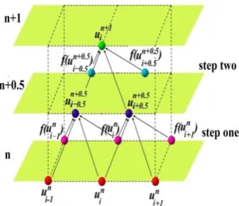
2. 2. Solution Procedures Computational grids consist of individual cells with spatial grid size ∆x and time steps ∆t (see Figure 3). In this study multi-step methods are used to enhance convergence and accuracy. The governing equations can be written in the following form:

(7)

where:

( _̇

)

(

_̇

̇ ₎

(8)

2. 2. 1. LxF Method The LxF method is the finite difference based numerical method appropriate for the solution of PDEs and prototype of most central schemes. The LxF method is conservative and monotone, therefore, this is a TVD (total variation diminishing) method. As for the original Godunov method, the LxF scheme is based on a piecewise constant approximation of the solution, but it does not require solving a Riemann problem for time advancing and only uses flux estimates.

LxF method is available for all forms of PDEs. The stability condition is

, where a is the corresponding wave speed.

In this scheme a half step is taken with LxF on a staggered mesh. If the second half step is taken with LxF, the solution is obtained on the original mesh.

Figure 3. Stencil for two time steps method

Figure 4. Stencil of conventional LxF method

Equation (7) is discretized in space with conventional LxF method [15]:

(9)

In Figure 4, stencil of conventional LxF is plotted. Considering Equation (9), we can discretize Equation (7) with the two-step variant of LxF method on the staggered grid. Accordingly, in the first step it arrives at:

(10)

(11)

Note that this step has to be applied to spatial nodes in time level .

In the second step, the unknown in the next time step is reached:

(12)

₍

)

(13)

In Figure 5, stencil of two-step LxF is plotted.

2. 2. 2. NT Method Actually the prototype of NT method is LxF scheme. The stability condition again is

. It is based on a staggered grid and uses the reconstruction of MUSCL-type piecewise linear interpolants in space, oscillation-suppressing nonlinear limiters, and the midpoint quadrature rule for evaluating integrals with respect to time. So we discretized Equation (7) with NT method on the staggered grid: First step:

* (

) ( )+

(14)

which . and as follows:

(15)

(16)

Use values to approximate the partial derivative scaled by ∆x with:

(17)

(18)

Here MM is the MinMod limiter which can be defined for two scalar arguments as:

( ) | | | | (19)

Thus and are:

(20)

(21)

This provides a piecewise constant approximation at time . The second step which is similar to the first step is calculated:

₍

) ( *

* (

) (

)+

(22)

which .

and

as follows:

(23)

(24)

If and , we have:

( * (25)

( * (26)

Previously function MM was defined in Equation (19). Thus and are:

( ) (27)

(

) (28)

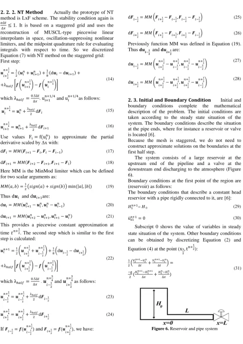
2. 3. Initial and Boundary Condition Initial and boundary conditions complete the mathematical description of the problem. The initial conditions are taken according to the steady state situation of the system. The boundary conditions describe the situation at the pipe ends, where for instance a reservoir or valve is located [6].

Because the mesh is staggered, we do not need to construct approximate solutions on the boundaries at the first half step.

The system consists of a large reservoir at the upstream end of the pipeline and a valve at the downstream end discharging to the atmosphere (Figure 6).

Boundary conditions at the first point of the region are (reservoir) as follows:

The boundary conditions that describe a constant head reservior with a pipe rigidly connected to it, are [6]:

= H 0 (29)

̇ (30)

Subscript 0 shows the value of variables in steady state situation of the system. Other boundary conditions can be obtained by discretizing Equation (2) and Equation (4) at the point ( ):

( )

(31)

(32) ( ) ( ) ̇ ̇ ̇ ̇ (33) ̇ _̇ ̇ ̇ (34)

This is known as the Mur boundary condition. In junction coupling, Poisson ratio is zero.

Boundary conditions at the end point of the region (valve) are as follows:

Junction coupling is a result of local forces on (from) pipe (fluid). Local forces act at specific points of a system, such as elbows, tees or valves, and cause a structural motion that can be regarded as a pumping action due to generating positive or negative pressure. It generates pressure waves in the fluid. The instantaneous closure of a valve which can move in the axial direction is modeled by:

_̇

₍₃₅₎

₍₃₆₎

where Af = cross-sectional discharge area and At= cross-sectional pipe wall area. Subscript M refers to the value of variables in valve. The boundary condition at the end point of the region can be derived similarly by discretizing Equation (1) and Equation (5) at the point ( ): ( ) ( ) (37) (38) ( ̇ ̇ ̇ _̇ * (39)

̇ ̇ ̇ ̇ (40)

Poisson coupling relates the pressures in the fluid to the axial stresses in the pipe via the contraction or expansion of the pipe wall. The boundary conditions describing the instantaneous closure of a valve rigidly connected to the ground are:

₍₄₁₎

̇ (42)

For calculation of , we can use Equation (1) and can be derived by discretizing Equation (4) at the point ( ):

( ) ( ) (43) (44) ( ) ( ) ̇ _̇ ̇ ̇ (45) ̇ _̇ ̇ ̇ (46)

Boundary conditions in Poisson and junction coupling are the same of junction coupling but with non-zero Poisson ratio.

3. VERFICATION OF NUMERICAL MODEL

reservoir-pipe-valve system (shown in Figure 6) considering the Poisson and junction coupling separately and their results are compared with MOC and Godunov solutions. Furthermore, test problem is solved with considering Poisson and junction coupling and its result is compared with results available in the literature [14]. The specifications of test problem are shown in Table 1.

Figure 7 displays the corresponding pressures considering Poisson and junction coupling at valve obtained with LxF and NT, respectively. In the first period, there is good agreement between results of LxF and NT with reference [14]. After the first period, curves of proposed methods are far from the results of reference [14]. It is noted that the benchmark problem is numerical test case only; experimental data do not exist [14].

In Figure 8, the time history of head with junction coupling is compared with results of MOC and Godunov schemes at valve. The head predictions of LxF and NT are in good agreement with results of MOC & Godunov schemes.

Time history of head with Poisson coupling is plotted in Figure 9, calculated using LxF and NT methods. It is seen that the results of proposed methods are in better agreement with results of Godunov scheme than results of MOC. At first, the LxF and NT methods are in good agreement with MOC but after first period, curves of proposed methods are far from results of MOC and with time, distances of the two curves increases.

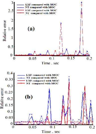
Figure 10 shows comparison of relative errors of LxF and NT methods with MOC and Godunov schemes for the case of junction coupling for two different courant numbers. The most accurate results of MOC occur in courant number 1. It is seen that the results of proposed methods, similar to Godunov scheme, are more accurate in courant number 0.9 in contrast with MOC scheme.

TABLE 1. Features of FSI problem (Delft Hydraulic

Benchmark problem A) [14]

Parameter Value

Length 20 (m)

Diameter 797 (mm)

Thickness 8 (mm)

Pipe’s density 7900 (kg/m3₎

Young’s modulus 210 (GPa)

Poisson’s ratio 0.3

Pressure wave speed 1024.7 (m/s)

Stress wave speed 5280.5 (m/s)

Steady state velocity 1 (m/s)

Reservoir head 0 (m)

Proposed methods are unable to simulate Poisson coupling in courant 1.

Figure 7. Comparison of simulations results of Delft

Hydraulics Benchmark problem A [14] for the end point (valve) pressure with results obtained by (a) LxF and (b) NT

Figure 8. Comparison of simulations results obtained by

MOC and Godunov schemes for the end point (valve) pressure

Figure 9. Comparison of simulations results obtained by MOC and Godunov schemes for the end point (valve) pressure

H for the Poisson coupling with (a) LxF and (b) NT

Figure 10. Comparison of relative error of LxF and NT with

MOC and Godunov for the case of junction coupling for courant number (a) C=1 and (b) C=0.9

Table 2 shows comparison of the maximum relative errors of LxF and NT with MOC and Godunov. LxF method can simulate junction coupling with less error than NT method compared to results of MOC. In contrast, when compared with the results of Godunov method, NT method simulated with less error than LxF method. For the case of Poisson coupling, LxF method can simulate more accurately than NT method compared with results of MOC and Godunov.

Table 3 shows run times for all methods considering the junction and Poisson coupling. It shows that proposed methods are really fast and lead to a considerable reduction in run times, as they do not require solving a Riemann problem for time advancing.

In addition to the above mentioned methods, we simulated FSI with MacCormac (MC) and two-step variant of the Lax-Wendroff (LxW) method (LxW) and the LxW method with a nonlinear filter (SLxW). Nonlinear filter reduced the total variation of the numerical solution. In junction coupling, MC and LxW and SLxW simulated FSI with a lot of fluctuations in heads in discontinuities. In Poisson coupling, these methods failed to predict heads in the example presented in this article [16].

TABLE 2. Comparison of the maximum relative error of LxF

and NT with MOC and Godunov

Max relative error

Method Junction

coupling

Poisson coupling

LXF

Compared to MOC 0.2812 0.8391

Compared to Godunov 0.3313 0.3475

NT

Compared to MOC 0.3273 0.8973 Compared to Godunov 0.0434 0.5836

TABLE 3. Comparison of the maximum relative error of LxF

and NT with MOC and Godunov

Godunov MOC

NT LXF Method

15 0.7

7.5 2.5 Junction couple Run

times

46 1.5

18 10.5 Poisson couple

4. SUMMARY AND CONCLUSIONS

proposed methods were compared with the results of solving MOC, Godunov schemes and exact solution of linear hyperbolic four-equation system in three mechanisms (Poisson coupling, junction coupling and Poisson and junction coupling). The obtained results showed that these schemes can predict head fluctuations and discontinuities with an acceptable order of accuracy in the FSI. In these schemes, no Riemann problems were solved and hence field-by-field decompositions were avoided which led to reduced run times. It is therefore suggested that, the LxF and NT are good alternatives for MOC and Godunov schemes when these methods face restrictions in FSI problems.

5. REFERENCES

1. Lefrançois, E. and Boufflet, J.-P., "An introduction to fluid-structure interaction: Application to the piston problem", SIAM Review, Vol. 52, No. 4, (2010), 747-767.

2. Wiggert, D., "Coupled transient flow and structural motion in liquid-filled piping systems: A survey", in Proc of ASME Pressure Vessels and Piping Conf., (1986).

3. Jain, M., Sharma, G. C. and Singh, A., "A mathematical model for blood flow through narrow vessels with mild-stenosis",

International Journal of Engineering Transactions B: Applications, Vol. 22, (2009), 307-315.

4. Wiggert, D. C. and Tijsseling, A. S., "Fluid transients and fluid-structure interaction in flexible liquid-filled piping", Applied Mechanics Reviews, Vol. 54, No. 5, (2001), 455-481. 5. Gale, J. and Tiselj I., "Godunov's method for stimulation of

fluid-structure interaction in piping systeams", Journal of Pressure Vessel Technology, Vol. 130, No. 3, (2008). 6. Lavooij, C. and Tusseling, A., "Fluid-structure interaction in

liquid-filled piping systems", Journal of Fluids and Structures,

Vol. 5, No. 5, (1991), 573-595.

7. Ahmadi, A. and Keramat, A., "Investigation of fluid–structure interaction with various types of junction coupling", Journal of Fluids and Structures, Vol. 26, No. 7, (2010), 1123-1141. 8. Liska, R., Shashkov, M. and Wendroff, B., "The early influence

of peter lax on computational hydrodynamics and an application of lax-friedrichs and lax-wendroff on triangular grids in lagrangian coordinates", Acta Mathematica Scientia, Vol. 31, No. 6, (2011), 2195-2202.

9. Tang, H.-Z. and Xu, K., "Positivity-preserving analysis of explicit and implicit lax–friedrichs schemes for compressible euler equations", Journal of Scientific Computing, Vol. 15, No. 1, (2000), 19-28.

10. Kao, C.Y., Osher, S. and Qian, J., "Lax–friedrichs sweeping scheme for static hamilton–jacobi equations", Journal of Computational Physics, Vol. 196, No. 1, (2004), 367-391. 11. Nessyahu, H. and Tadmor, E., "Non-oscillatory central

differencing bolic conservation laws", Journal of Computational Physics, Vol. 87, (1990), 159-193.

12. Arminjon, P. and St-Cyr, A., "New space staggered and time 2nd order finite volume methods", Hyperbolic Problems: Theory, Numerics, Applications, (2003), 295-304.

13. Naidoo, R. and Baboolal, S., "Numerical integration of the plasma fluid equations with a modification of the second-order nessyahu–tadmor central scheme and soliton modeling",

Mathematics and Computers in Simulation, Vol. 69, No. 5, (2005), 457-466.

14. Tijsseling, A., "Exact solution of linear hyperbolic four-equation system in axial liquid-pipe vibration", Journal of Fluids and Structures, Vol. 18, No. 2, (2003), 179-196.

15. Hoffmann, K.A. and Chiang, S.T., "Computational fluid dynamics for engineers", Engineering Education Systems, Austin, Texas, USA, (1989).

Investigation of Fluid-structure Interaction by Explicit Central Finite Difference

Methods

F. Khalighia_{, A. Ahmadi}a_{, A. Keramat}b

a _{Department of Civil Engineering, Shahrood University of Technology, Shahrood, Iran} b _{Department of Civil Engineering, Jundi-shapur University of Technology, Dezful, Iran}

P A P E R I N F O

Paper history:

Received 23September 2015

Received in revised form 27February 2016 Accepted 04 March 2016

Keywords:

Fluid-structure Interaction Lax-Friedrichs Method Nessyahu-Tadmor Method Water Hammer

ديكچ ه

یه دراٍ ِلَل ُسبس ِث یْجَت لثبق یکیهبٌید یبٍّزیً ،چَق ِثزض ُذیذپ يیح رد تکزح ثعبث بٍّزیً يیا ِچًبٌچ ،دَض

ٍ

لکض زییغت ِلَل ِکجض ُذیذپ ،ذًَض لبیس لخاذت مبً ِث یا

-ُسبس (

FSI

) خر ذّاَخ داد لبیس یلخاذت ثحبجه .

ذًٌبه ،ُسبس

تا ٍ يساَپ ِلپَک ىآ تازثا ٍ لبص

چَق ِثزض ُذیذپ جیبتً زث بّ ترَص ِث تازثا يیا ازیس تسا ُدَث ِجَت درَه ُراَوّ

دبجیا ىبسًَ صیاشفا ٍ ِثبج يیٌچوّ ٍ ربطف یبّذّ رد ییبج

یه ُذّبطه ِلَل ُراَید .دَض

زث نکبح تلادبعه سا ُذیذپ يیا

عًَ ییشج لیسًازفید تلادبعه یَلَلذّ

لٍا ِجتزه یه ذٌضبث ُسبس ٍ یکیلٍرذیّ تلادبعه ِتسد ٍد ِث ٍ یه نیسقت یا

َض ً .ذ

لبیس صٌکرذًا ُذیذپ یسبسلذه رَظٌه ِث زضبح قیقحت رد

-ىشخه نتسیس کی رد ُسبس

-ِلَل -شٍر ،زیض یًبهس مبگٍد یبّ

سکلا -صیردزف

(LxF)

َّبیسً زث یٌتجه یضٍر ٍ

رَهدبت

(NT)

ٌس تحص رَظٌه ِث .تسا ِتفزگ رازق ُدبفتسا درَه ،یج

شٍر سا ُذهآ تسذث جیبتً بث شٍر ٍد يیا سا لصبح یدذع جیبتً ( ِصخطه طَطخ یبّ

(MOC

قیقد لح ٍ ًٍَدَگ ،

شٍر ِک دَوً تثبث جیبتً .تفزگ رازق ِسیبقه درَه یطخ یَلَلذّ ِلدبعه ربْچ نتسیس یبّ

LxF

ٍ

NT

لثبق تقد بث

یه یسبسلذه ار لبیس ربطف رد دَجَه یگتسَیپبً ،یلَجق .ذٌٌک

مبگ ُساذًا یگتسثاٍ مذع شٍر رد یًبکه ٍ یًبهس یبّ

یبّ

مبگ ةبختًا ىبکها ،ُذض ِتفزگربک ِث یه ار صخطه یًبهس مبگ کی یاسا ِث فلتخه یًبکه یبّ

تقد صیاشفا تجس ِک ذّد

یه ِصخطه طَطخ لَوعه شٍر ِث تجسً یسبسلذه شٍر يیا رد زگید ییَس سا .دَض

سا ىبویر ِلئسه لح مذع تلع ِث بّ

ِیحبً ِیشجت -یه یراددَخ ِیحبً یه ًٍَدَگ شٍر بث ِسیبقه رد لح ىبهس تذه صّبک ِث زجٌه ِک دَض

.دَض