A Consistent Information Criterion for Support Vector
Machines in Diverging Model Spaces
Xiang Zhang [email protected]
Yichao Wu [email protected]
Department of Statistics
North Carolina State University Raleigh, NC 27695, USA
Lan Wang [email protected]
Department of Statistics The University of Minnesota Minneapolis, MN 55455, USA
Runze Li [email protected]
Department of Statistics and The Methodology Center The Pennsylvania State University
University Park, PA 16802-2111, USA
Editor:Jie Peng
Abstract
Information criteria have been popularly used in model selection and proved to possess nice theoretical properties. For classification, Claeskens et al. (2008) proposed support vector machine information criterion for feature selection and provided encouraging numerical evidence. Yet no theoretical justification was given there. This work aims to fill the gap and to provide some theoretical justifications for support vector machine information criterion in both fixed and diverging model spaces. We first derive a uniform convergence rate for the support vector machine solution and then show that a modification of the support vector machine information criterion achieves model selection consistency even when the number of features diverges at an exponential rate of the sample size. This consistency result can be further applied to selecting the optimal tuning parameter for various penalized support vector machine methods. Finite-sample performance of the proposed information criterion is investigated using Monte Carlo studies and one real-world gene selection problem. Keywords: Bayesian Information Criterion, Diverging Model Spaces, Feature Selection, Support Vector Machines
1. Introduction
number of probes (or genes) can be tens of thousands and the number of patient samples is typically only a few dozens, biologists find it plausible to assume that only a small subset of genes are relevant. In this case, it is more desirable to build a classifier based only on those relevant genes. Yet in practice, it is largely unknown which genes are relevant and this calls for feature selection methods. The potential benefits of feature selection include reduced computational burden, improved prediction performance and simple model interpretation. See Guyon and Elisseeff (2003) for more discussions. Our goal in this paper is consistent feature selection for the SVM.
There has been a rich literature on feature selection for the SVM. Weston et al. (2000) proposed a scaling method to select important features. Guyon et al. (2002) suggested the SVM recursive feature elimination (SVM RFE) procedure. It has been shown that the SVM can be fitted in the regularization framework using the hinge loss and theL2 penalty (Wahba et al., 1999). Thereafter various forms of penalized SVMs have been developed for simultaneous parameter estimation and feature selection. Bradley and Mangasarian (1998), Zhu et al. (2004) and Wegkamp and Yuan (2011) studied properties of the L1 penalized SVM. Wang et al. (2006) proposed SVM with a combination of L1 and L2 penalties. Zou and Yuan (2008) considered theL∞penalized SVM when there is prior knowledge about the grouping information of features. Zhang et al. (2006) and Becker et al. (2011) suggested SVM with a non-convex penalty in the application of gene selection. Though all these methods target selecting the best subset of features, theoretical justification about how well the selected subset is estimating the true model is still largely underdeveloped. Recently Zhang et al. (2014) showed that the SVM penalized with a class of non-convex penalties enjoys the oracle property (Fan and Li, 2001), that is, the estimated classifier behaves as if the subset of all relevant features is known a priori. Yet this model selection consistency result relies heavily on the proper choice of the involved tuning parameter which is often selected by cross-validation in practice. However, Wang et al. (2007) showed that the generalized cross-validation criterion can lead to overfitting even with a very large sample size.
Information criteria such as AIC (Akaike, 1973) and BIC (Schwarz, 1978) have been used for model selection and their theoretical properties have been well studied, see Shao (1997), Shi and Tsai (2002) and references therein. It is well understood that the BIC can identify the true model consistently when the dimensionality is fixed. The idea of combining information criterion with support vector machine to select relevant features was first pro-posed in Claeskens et al. (2008). They propro-posed the SVM information criterion (SVMICL) and provided some encouraging numerical evidence. Yet its theoretical properties, such as model selection consistency, have not been investigated.
spaces the probabilities for favoring an underfitted or overfitted model by the information criterion can accumulate at a very fast speed and alternative techniques are required. We develop the uniform consistency of SVM solution which has not been carefully studied in the literatures. Based on the uniform convergence rate, we prove that the new information criterion possesses model selection consistency even when the number of features diverges at an exponential rate of the sample size. That is, with probability arbitrarily close to one, we can identify the true model from all the underfitted or overfitted models in the diverging model spaces. To the best of our knowledge, this is the first result of model selec-tion consistency for the SVM. We further apply this informaselec-tion criterion to the problem of tuning parameter selection in penalized SVMs. The proposed support vector machine information criterion can be computed easily after fitting the SVM with computation cost much lower than resampling methods like cross-validation. Simulation studies and real data examples confirm the superior performance of the proposed method in terms of model selection consistency and computational scalability.
In Section 2 we define the support vector machine information criterion. Its theoretical properties are studied in Section 3. Sections 4 and 5 present numerical results on simula-tion examples and real-world gene selecsimula-tion datasets, respectively. We conclude with some discussions in Section 6.
2. Support vector machine information criterion
In this paper we use normal font for scalars and bold font for vectors or matrices. Consider a random pair (X, Y) with XT = (1, X1, . . . , Xp) = (1,(X+)T)∈R(p+1) and Y ∈ {1,−1}. Let {(Xi, Yi)}n
i=1 be a set of training data independently drawn from the distribution of (X, Y). Denoteβto be a (p+ 1)-dimensional vector of interest withβT = (β0, β1, . . . , βp) = (β0,(β+)T) ∈ R(p+1). Let || · || be the Euclidean norm operator of a vector. The goal of linear SVM is to estimate a hyperplane defined by XTβ = 0 via solving the optimization problem
min
β
C n
X
i=1 ξi+1
2||β
+||2 (1)
subject to the constraints thatξi ≥0 andYiXTi β≥1−ξi for alli= 1, . . . , n, whereC >0 is a tuning parameter. This can be written equivalently into an unconstrained regularized empirical loss minimization problem:
min
β 1
n n
X
i=1
H(YiXTi β) + λn
2 ||β
+||2 , (2)
where H(t) = (1−t)+ is the hinge loss function, (z)+ = max(z,0) andλn>0 is a tuning parameter with C= (nλn)−1.
Following the definition in Koo et al. (2008), we denote (β∗)T = (β0∗, β1∗, . . . , βp∗) = (β∗0,(β∗+)T)∈R(p+1) to be the true parameter value that minimizes the population hinge loss. That is,
β∗= arg min
β E(1−YX
Note thatβ∗is not necessarily always the same as the Bayes rule. However, it gives the opti-mal upper bound of the risk of the 0-1 loss through convex relaxation and its sparsity struc-ture is exactly the same as the one of Bayes rule in special cases such as linear discriminant analysis. For more discussions see Zhang et al. (2014). DenoteS={j1, . . . , jd} ⊂ {1, . . . , p} to be a candidate model,XTi,S= (1, Xi,j1, . . . , Xi,jd),βTS = (β0, βj1, . . . , βjd) and|S|the car-dinality ofS. The subset of all relevant features is defined by S∗={j: 1≤j≤p, βj∗ 6= 0}. We assume that the truth β∗ is sparse (i.e., most of its components are exactly zero). De-note q =|S∗| which characterizes the sparsity level. We assume that q is fixed and does not depend on n. In this paper, we consider the diverging model spaces in which the di-mensionality p=pn is allowed to increase with nand can be potentially much larger than n. We also assume thatλn→0 asn→ ∞and only consider the non-separable case in the limit to ensure the uniqueness of the truth β∗. Here by non-separable, we mean that the two classes cannot be linearly separated from each other.
To identify the true modelS∗, Claeskens et al. (2008) proposed an information criterion for SVM (denoted by SVMICL) based on the slack variables{ξi}ni=1. That is,
SVMICL(S) = n
X
i=1
ξi+|S|log(n),
where{ξi}ni=1are obtained from (1) only using the variables inS. This information criterion is equivalent to
SVMICL(S) = n
X
i=1
(1−YiXTi,SβbS)++|S|log(n), (3)
where βbS = arg min{1/n Pn
i=1(1−YiXTi,SβS)+ +λn/2||β+S||2}. It is evident that the SVMICL directly follows the spirit of BIC. Claeskens et al. (2008) fixed C = 1 in (1) and found minor difference for different choices of C, which is equivalent to λn = 1/n in (2). To be consistent with the work in Claeskens et al. (2008), we also consider this choice of λn in this paper. There are two potential drawbacks of this information criterion. First, though supported with numerical findings, theoretical properties of SVMICL, such as model selection consistency, are largely unknown even under the assumption of a fixed p. Second, in many real world datasets where the dimension can be much larger than the sample size, it would be more appropriate to consider the model selection problem in the framework of diverging model spaces. This extension from low dimensions to high dimen-sions can greatly change the theoretical properties of the information criterion. Chen and Chen (2008) showed that the ordinary BIC for linear regression cannot identify the true model consistently in the diverging p case. Wang et al. (2009) showed that the ordinary BIC fails to select a consistent shrinkage level in penalized least squares regression with a diverging p. Such results in the literature suggest that SVMICL may also suffer from inconsistency in high dimensions and alternative criterion is needed.
To overcome these issues, we propose a modified support vector machine information criterion for model selection in a high dimensional model space (denote by SVMICH). This criterion is adpated from SVMICLand defined as
SVMICH(S) = n
X
i=1
whereβbS = arg min{1/n Pn
i=1(1−YiXTi,SβS)++λn/2||β+S||2}andLnis a constant sequence that diverges to infinity. Note that if Ln is a non-diverging constant then this reduces to SVMICL in the limit. We will show that SVMICH possesses the nice property of model se-lection consistency even whenpincreases at an exponential rate ofn. Compared to SVMICL in Claeskens et al. (2008), our information criterion SVMICH adds larger penalty to the size of the selected subset and behaves more conservatively. As we will see, this additional preference for simpler models plays an important role in consistent model selection when we are searching over diverging model spaces.
We make two remarks about SVMICH. First, the choice ofLnin (4) is flexible. It isnot a tuning parameter and does not need to be chosen by computationally intensive methods such as cross-validation. We will show that a wide spectrum ofLn can lead to a consistent information criterion. This is further confirmed in our simulations and real data analysis where we examine different choices of Ln. Therefore the computation cost of SVMICH is the same as SVMICL and much lower than cross-validation. Second, it is possible to define the information criterion as the log-transformed version, that is
log( n
X
i=1
(1−YiXTi,SβbS)+) +Ln|S|log(n)/n
which is scalar invariant. It can be shown the model selection consistency still holds for this definition. However, we follow the advice from Guyon et al. (2002) to standardize variables before training SVM and as a consequence we automatically have scalar invariance of the sum of slack variables. To be consistent with SVMICL defined in Claeskens et al. (2008), we take definition (4) in our paper.
3. Theoretical results
3.1 Notations and conditions
To facilitate technical proofs, we introduce some additional notation. DenoteL(β) =E(1−
YXTβ)
+. Recall that β∗ = arg minβL(β). Let S(β) =−E[1(1−YXTβ≥0)YX], where
1(·) is the indicator function. Also define H(β) =E[δ(1−YXTβ)XXT], where δ(·) is the
Dirac delta function. Koo et al. (2008) showed that under some regularity conditions,S(β) and H(β) behave like the gradient and Hessian matrix of L(β), respectively. Furthermore we denotef+ and f− to be the densities of X+ ∈Rp conditioning on Y = 1 and Y =−1, respectively.
Given the dimension p, the number of candidate models is 2p−1. Whenpis very large, we cannot afford to calculate SVMICH(S) for all possible subsets. Instead, we only search for the best model in a restricted model space. To be more specific, we denoteSbthe model
chosen by SVMICH such that
b
S= arg minS:|S|≤MnSVMICH(S), (5)
Note that by Lemma 1 of Zhang et al. (2014), if the number of relevant features diverges faster than√n, the true parameterβ∗cannot be estimated consistently even with the oracle information of the true modelS∗. Therefore, there is no need to consider those models with sizes increasing faster than√nas in general no method would work for them even when the true underlying model is known. Notice also that it is possible to prove the model selection consistency without the restricted model space. However, this would requirespn=o(
√ n), which cannot diverge very fast with the sample size.
We now present the technical conditions that are needed for studying the theoretical properties of SVMICH .
(A1) f+ and f− are continuous and have some common support in Rp. (A2) |Xj| ≤M <∞for some positive constant M and 1≤j≤p.
(A3) For all S∈ {S :|S| ≤Mn, S ⊇S∗},λmax(E(Xi,SXTi,S))≤c1, where λmax(·) is the largest eigenvalue of a matrix andc1 >0 is a constant.
(A4) The densities of XTi,S∗β∗S∗ conditioning on Y = 1 and Y = −1 are uniformly bounded away from zero and infinity at the neighborhood ofXTi,S∗β∗S∗ = 1 andXTi,S∗β∗S∗=
−1, respectively.
(A5) Mn=O(nκ) for some constant 0< κ <1/2.
(A6) pn=O(exp(nγ)) for some constant 0< γ <(1−2κ)/5.
(A7) For all S ∈ {S :|S| ≤Mn, S ⊇S∗}, there exist some positive constants c2 and c3 such that λmin(H(βS))≥c2 and λmax(H(βS)) =O(|S|) over the set {β:||β−β∗|| ≤c3}, whereλmin(·) is the smallest eigenvalue of a matrix.
(A8) For all S ∈ {S : |S| ≤ Mn, S ⊇ S∗}, λmax(H(β∗S)) log(pn) = o(Lnlog(n)), Lnlog(n) =o(n).
Conditions (A1) is required so that S(β) and H(β) are well-defined, see Koo et al. (2008) for more details. Condition (A2) is assumed in the literature of high dimensional model selection consistency as in Wang et al. (2012) and Lee et al. (2014). Condition (A3) on the largest eigenvalue is similar to the sparse Riesz condition (Zhang and Huang, 2008) and is often assumed for model selection consistency in the divergingpscenario (Chen and Chen, 2008; Yuan, 2010; Zhang, 2010). Note that the lower bound on the eigenvalue of the covariance matrix of XS is not specified. Condition (A4) assumes that as the sample size increases, there is enough information around the non-differentiable point of the hinge loss function. This condition is also required for model selection consistency of non-convex penalized SVM in high dimensions (Zhang et al., 2014). Condition (A6) specifies thatp is allowed to diverge at an exponential rate of n. Conditions (A7) requires that the Hessian matrix is well-behaved. More specifically, (A7) requires a lower bound on the smallest eigenvalue of the Hessian matrix in the neighborhood of the true value. Koo et al. (2008) gave sufficient conditions for the positive-definiteness of the Hessian matrix at the true value and showed these conditions hold under the setting of Fisher’s linear discriminant analysis with a fixed model size. Condition (A8) specifies the rate requirement ofLn in (4).
3.2 Consistency of SVMICL for a fixed p
Note that, to prove the model selection consistency of SVMICL, we need to show that
Pr( inf
S∈Ω,S6=S∗SVMICL(S)>SVMICL(S ∗
))→1
as n → ∞. By the fact that Ω is a fixed model space, it is sufficient to show the result point-wisely in the model space, that is,
Pr(SVMICL(S)>SVMICL(S∗))→1 (6)
for every S ∈ {S : S ∈ Ω, S 6= S∗}. This point-wise version greatly simplifies the proof. Recall thatβbS = arg min{1/n
Pn
i=1(1−YiXTi,SβS)++λn/2||β+S||2}. As we will show in the appendix, it suffices to conclude (6) with the condition that βbS is a consistent estimator
of β∗S whenever the candidate subsetS includes the true subsetS∗. By Theorem 1 of Koo et al. (2008), we have||βbS−β∗S||=Op(n−1/2) for every fixed S⊃S∗under the assumption
of fixedp. Therefore the point-wise consistency holds. The result is summarized in Lemma 1.
Lemma 1 Assuming p is a fixed number and λn= 1/n. Under conditions (A1)-(A4) and
(A6)-(A7), we have
Pr(Sb=S∗)→1
as n→ ∞, where Sb= arg minS:|S|≤MSVMICL(S).
3.3 Consistency of SVMICH for a diverging p
The proof becomes much more involved when p is diverging, especially when p diverges much faster than O(√n). Let Ω ={S :|S| ≤Mn}, Ω+ ={S :|S| ≤ Mn, S ⊃S∗, S 6=S∗} and Ω− = {S : |S| ≤ Mn, S 6⊃ S∗}, where Ω+ and Ω− are spaces of overfitted and un-derfitted models, respectively. Though the information criterion for the fixed model space can differentiate the true model from an arbitrary candidate model, this point-wise result is not sufficient for the overall consistency if the problem requires searching uniformly over a diverging model space. That is, even if (6) holds for everyS∈Ω, we still cannot conclude model selection consistency, as the probability of favoring an overfitted or underfitted can-didate model rather than the true model can accumulate at very fast speed if the number of candidate models is diverging and hence lead to inconsistent model selection. To control the overall failing probability, we need a uniform convergence rate of SVM solutionβbS over
the diverging model space Ω. Note that Ω = Ω+∪ {S∗} ∪Ω−. It turns out that the uniform convergence rate ofβbS overS ∈Ω+ is sufficient for the technical proof. We summarize the
uniform rate in Lemma 2 below.
Lemma 2 Under conditions (A1)-(A7) and λn= 1/n, we have
sup S:|S|<Mn,S⊃S∗
||βbS−β∗S||=Op( p
|S|log(p)/n).
This uniform convergence rate of SVM solution is far from being a trivial result. Recently Zhang et al. (2014) showed that||βbS−β∗S||=Op(
p
et al. (2008) to the divergingpcase, it is still only a point-wise result and cannot be applied directly to bound the overall failing probability. Not surprisingly, the uniform convergence rate in Lemma 2 is slower by a factor plog(p), which is the price we pay to search over the candidate model space uniformly. In fact, this additional term is the main reason for adding the extra penalty Ln in SVMICH.
We now give an intuitive explanation why SVMICL can fail in the diverging model space. Consider all the overfitted models in Ω+. We have the following decomposition
inf S∈Ω+
SVMICL(S)−SVMICL(S∗)
= inf S∈Ω+
n
X
i=1
(1−YiXTi,SβbS)+−
n
X
i=1
(1−YiXTi,S∗β∗S)++ (|S| − |S∗|) log(n) . (7)
Note that the difference of the sum of hinge loss can be negative and the difference of model size is always positive. We will show in the appendix that the difference of the sum of hinge loss is of order Op(n||βbS−β∗S||2) under some regularity conditions. For fixed p, it
implies that the difference of model size dominates for largenand the sign of (7) is always positive in the limit. For diverging p, however, this is not always the case. By Lemma 2, the difference of hinge loss in (7) is of orderO(|S|log(p)) and the difference of model size is of orderO(|S|log(n)), thus the sign of (7) can be negative in the limit. Therefore even if we have a very large sample size, SVMICLmay still favoring the models that are overfitted due to the slower uniform convergence rate of SVM solution. Because SVMICL can be viewed as directly following the spirit of ordinary BIC, this result agrees with the findings reported in Chen and Chen (2008) that BIC can be too liberal in high dimensional model selection. Here by liberal, we mean that there is a positive probability that an overfitted model is more favored than the true model by the information criterion even with an infinite sample size.
For SVMICH, we can do a similar decomposition as in (7) for all the overfitted models
inf S∈Ω+
SVMICH(S)−SVMICH(S∗)
= inf S∈Ω+
n
X
i=1
(1−YiXTi,SβbS)+−
n
X
i=1
(1−YiXTi,S∗β∗S)++Ln(|S| − |S∗|) log(n) . (8)
Note that the extra termLndiverges to infinity and the sign of (8) in the limit is determined by the difference of model size, which is always positive. That is, SVMICH can identify the true model from all the overfitted models for sufficiently largen. This result is summarized in Lemma 3.
Lemma 3 Under conditions (A1)-(A8) and λn= 1/n, we have
Pr( inf S:S∈Ω+
SVMICH(S)>SVMICH(S∗))→1.
as n→ ∞.
difference of the model size|S| − |S∗|can be negative and thus the decomposition in (7) is not helpful. However, one can always add relevant features to the underfitted model and study the enlarged model instead. To be more specific, for every S ∈Ω−, one can always create the enlarged model ˜Ssuch that ˜S =S∪S∗. Note that ˜S is either an overfitted model or the true model. The model ˜S which includes all the signals bridges the underfitted and overfitted model space through the simple fact
inf S:S∈Ω−
SVMICH(S)−SVMICH(S∗)
= inf S:S∈Ω−
{[SVMICH(S)−SVMICH( ˜S)] + [SVMICH( ˜S)−SVMICH(S∗)]}.
By Lemma 3, in the limit the difference SVMICH( ˜S)−SVMICH(S∗) is non-negative for everyS ∈Ω−(could be exactly 0). Note also that the difference betweenSand ˜S is at least one missing relevant feature. According to the assumption that the signals do not diminish to 0 as sample size increases, one can show the model with more signals always produces a strictly smaller sum of hinge loss in the limit. That is, for sufficiently large n, we always have
n
X
i=1
(1−YiXTi,SβbS)+−
n
X
i=1
(1−YiXTi,S˜βb˜
S)+ ≥C >0
for every S ∈ Ω− and some constant C does not depend on S. Then we arrive at the following result for the underfitted model space.
Lemma 4 Under conditions (A1)-(A8) and λn= 1/n, we have
Pr( inf S:S∈Ω−
SVMICH(S)>SVMICH(S∗))→1.
as n→ ∞.
By combing Lemma 3 and Lemma 4, we can conclude the model selection consistency of SVMICH in the diverging model space.
Theorem 5 Under conditions (A1)-(A8) andλn= 1/n, we have
Pr( ˆS =S∗)→1.
as n, p→ ∞, where Sb= arg minS:|S|≤MnSVMICH(S).
3.4 Application to tuning parameter selection in penalized SVMs
Theorem 1 states that SVMICH can identify the true model from Ω. However, in practice it can be very time-consuming and even infeasible to calculate SVMICH(S) for everyS ∈Ω. One possible approach is to form a solution path via penalized SVM and only consider the candidate models on the path. The idea of using solution path has been shown to greatly reduce the computation burden, see Mazumder et al. (2011). For the solution path of penalized SVM, Hastie et al. (2004) studied the L1 penalized SVM and showed that the solution path is piece-wise linear in C which is the regularization parameter in (1).
on the BIC-type information criterion, including Wang et al. (2009) for penalized linear regression, Kawano (2012) for bridge regression, Lee et al. (2014) for penalized quantile regression and Fan and Tang (2013) for penalized generalized linear model. Following the ideas therein, we propose to choose the shrinkage level of penalized SVMs based on the
modified support vector machine information criterion. Let βb
T
λn = ( ˆβλn,0,βλn,1, . . . ,ˆ βλn,p)ˆ be the solution to some penalized SVM with a tuning parameterλn. That is,
b
βλn = arg min
β 1
n n
X
i=1
(1−YiXTi β)++ p
X
j=1
pλn(βj) , (9)
where pλn(·) is some penalty function with a tuning parameter λn. Denote Sbλn ={j : 1≤
j≤p,βλn,jˆ 6= 0}. We define the information criterion for choosing tuning parameterλn as
SVMICH(λn) = n
X
i=1
(1−YiXTi βbλn)++Ln|Sλnb |log(n),
whereLnis defined in SVMICH(S). The selected tuning parameter is the one that minimizes the information criterion and results in the model size within the restricted model space, that is,
b
λn= arg min λ:|Sbλ|≤Mn
SVMICH(λ).
This information criterion for selecting tuning parameter can be applied to various penalized approaches for sparse SVMs. Note that the feature selection consistency of the SCAD penalized SVM is shown to rely on the proper choice of the tuning parameter (Zhang et al., 2014), where resampling procedure such as five-fold cross-validation is commonly used in practice. As we will also show in our numerical findings in Section 4.2, the proposed information criterion SVMICH(λn) usually select the shrinkage level that leads to the correct model size. The tuning parameter selected by cross-validation, however, is more likely to be under-penalized and lead to an overfitted model. Furthermore, the cross-validation is more computationally intensive than information criterion and hence less desirable when the number of features is large.
4. Simulations
In this section we study the finite-sample performance of SVMICH. We are interested in the model selection ability of SVMICH(S) and the tuning parameter selection ability of SVMICH(λn). We also examine the effect of different choices of Ln in the definition of SVMICH. For all simulations, we consider the rates log(log(n)), plog(n), log(n) and n−1/3 for Ln. We compare with SVMICL in Claeskens et al. (2008) and the extended Bayesian information criterion (EBIC) proposed in Chen and Chen (2008). Note that EBIC is originally proposed for model selection in the diverging model space in the framework of regression and it has not been applied into classification problem. However, the main strategy therein is to add an additional term log( |Sp|
) log(n) in the BIC penalty, where p
|S|
selection of SVM by selecting the model S that minimizes the criterion
n
X
i=1
(1−YiXTi,SβbS)++|S|log(n) + log
p
|S|
log(n).
This modification essentially follows the idea in Chen and Chen (2008) and we are interested in its finite-sample performance compared with SVMICH.
To investigate these issues, we conduct the SCAD penalized SVM, which has been shown to enjoy the model selection consistency for a properly chosen tuning parameter (Zhang et al., 2014). That is, given a specificλn, we solve (9) with pλn(·) being the SCAD penalty defined in Fan and Li (2001). The corresponding optimization problem is a non-convex one, for which the local linear approximation (LLA) algorithm (Zou and Li, 2008) is implemented in all our numerical studies. To be more specific, for step t≥1, given the
solution βb
(t−1)
= ( ˆβ0(t−1), . . . ,βˆp(t−1))T at the previous step, we update by solving
b
β(t)= arg min
β {
1 n
n
X
i=1
(1−YiXTiβ)++ p
X
j=1
pλn0 (|βˆj(t−1)|)|βj|},
wherep0λn(·) denotes the derivative ofpλn(·). Note that each update step can be easily recast as a linear programming (LP) problem and efficiently solved by many popular solvers. In
this paper we take the initial value{βb
(0)
: ˆβ(0)j = 0,0≤j≤p} and claim convergence if the value||βb
(t−1) −βb
(t)
||is small enough.
4.1 Model selection of SVMICH(S)
In this subsection we study the model selection ability of SVMICH(S). The data are generated from two models. The first model is adapted from Fisher’s linear discriminant analysis (LDA) and the second model is related to probit regression.
• Model 1: Pr(Y = 1) = Pr(Y = −1) = 0.5, X|(Y = 1) ∼ M N(µ,Σ), X|(Y = −1)∼M N(−µ,Σ),q = 4,µ= (0.25,0.25,0.25,0.25,0, . . . ,0)T ∈Rp,Σ= (σij) with nonzero elements σii = 1 for i= 1,2,· · · , pand σij =ρ = −0.2 for 1 ≤ i6= j ≤ q. The Bayes rule is given by sign(X1+X2+X3+X4) with Bayes error 21.4%.
• Model 2: X∼M N(0p,Σ),Σ= (σij) with nonzero elementsσii= 1 fori= 1,2,· · ·, p and σij = ρ = 0.4|i−j| for 1 ≤ i 6= j ≤ q, Pr(Y = 1) = Φ(XTβ) where Φ(·) is the CDF of the standard normal distribution,q= 4,β= (0.8,0.8,0.8,0.8,0, . . . ,0)T. The Bayes rule is sign(0.57X1+0.34X2+0.34X3+0.57X4) with Bayes error 11.5%.
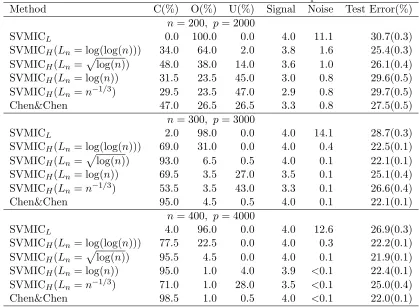
“Overfit” summarize the percentages over 200 replications for correct model selection, over-fitting and underover-fitting, respectively. The numbers under columns “Signal” and “Noise” are the average numbers of selected relevant and irrelevant features, respectively. We also generate an independent dataset with sample size 10000 to evaluate the test error. Numbers in parentheses are the corresponding standard errors.
Table 1 summarizes the model selection results of SVMICL, SVMICH and the criterion proposed in Chen and Chen (2008) for Model 1. For all (n, p) combinations, SVMICH shows uniformly higher percentages to identify the correct model than SVMICL regardless of the choices of Ln. It can be seen that in the cases p is much larger than n, SVMICL behaves too liberal and tends to select an overfitted model. Note that SVMICH also has a significantly lower testing error than SVMICL in all settings even when SVMICL includes slightly more signals in the model. This agrees with the findings in Fan and Fan (2008) that the accumulation of the noises can greatly blur the prediction power. Though the SVMICH with differentLn all performs better than SVMICL, their performances are not exactly the same. For the criteria with a more aggressive penalty on the model size such as log(n) and n−1/3, there are considerable underfitting when the sample size is small (n = 200). As the sample size increases, the difference of Ln decreases. This suggests that although asymptotically the choice ofLn can lie in a wide range of spectrums, for small sample sizes some choices of Ln can be too conservative and may not be much better than SVMICL which is too liberal. In general, we find Ln=plog(n) seems to be a reasonable choice for many scenarios.
Another interesting finding is the comparison to the criterion following the spirit in Chen and Chen (2008). Though its theoretical property has not been investigated, the empirical results suggest that it performs similar to SVMICH with Ln =plog(n) in finite samples. In fact, by using the approximation that |Sp|
≈ p|S| when p is much larger than|S|, one can easily show that
log(n)|S|log(log(n))<log(n)|S|+ log(n) log
p |S|
<log(n)|S|log(n)
forn < p <103nand a very wide range ofn. This provides some evidence that the criterion directly adapted from Chen and Chen (2008) behaves more libearal than SVMICH with Ln= log(n) but is more aggressive than SVMICH with Ln= log(log(n)).
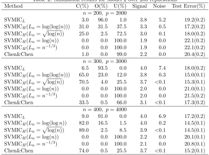
Table 2 summarizes the model selection results for Model 2. The SVMICH with log(log(n)) and plog(n) as Ln perform uniformly better than SVMICL and the criterion in Chen and Chen (2008) for all scenarios. Due to the correlations among the signals, the more aggressive choices of Ln suffer from considerable underfitting. Again our empirical results suggest that Ln =
p
log(n) seems to be an appropriate choice for a wide range of problems.
4.2 Tuning parameter selection of SVMICH(λ)
In this subsection we examine the tuning parameter selection ability of SVMICH(λ). The data is generated from the following model.
Table 1: Simulation results for Model 1 over 200 replications
Method C(%) O(%) U(%) Signal Noise Test Error(%) n= 200, p= 2000
SVMICL 0.0 100.0 0.0 4.0 11.1 30.7(0.3) SVMICH(Ln= log(log(n))) 34.0 64.0 2.0 3.8 1.6 25.4(0.3) SVMICH(Ln=plog(n)) 48.0 38.0 14.0 3.6 1.0 26.1(0.4) SVMICH(Ln= log(n)) 31.5 23.5 45.0 3.0 0.8 29.6(0.5) SVMICH(Ln=n−1/3) 29.5 23.5 47.0 2.9 0.8 29.7(0.5) Chen&Chen 47.0 26.5 26.5 3.3 0.8 27.5(0.5)
n= 300, p= 3000
SVMICL 2.0 98.0 0.0 4.0 14.1 28.7(0.3) SVMICH(Ln= log(log(n))) 69.0 31.0 0.0 4.0 0.4 22.5(0.1) SVMICH(Ln=
p
log(n)) 93.0 6.5 0.5 4.0 0.1 22.1(0.1) SVMICH(Ln= log(n)) 69.5 3.5 27.0 3.5 0.1 25.1(0.4) SVMICH(Ln=n−1/3) 53.5 3.5 43.0 3.3 0.1 26.6(0.4) Chen&Chen 95.0 4.5 0.5 4.0 0.1 22.1(0.1)
n= 400, p= 4000
SVMICL 4.0 96.0 0.0 4.0 12.6 26.9(0.3) SVMICH(Ln= log(log(n))) 77.5 22.5 0.0 4.0 0.3 22.2(0.1) SVMICH(Ln=
p
log(n)) 95.5 4.5 0.0 4.0 0.1 21.9(0.1) SVMICH(Ln= log(n)) 95.0 1.0 4.0 3.9 <0.1 22.4(0.1) SVMICH(Ln=n−1/3) 71.0 1.0 28.0 3.5 <0.1 25.0(0.4) Chen&Chen 98.5 1.0 0.5 4.0 <0.1 22.0(0.1)
elements σii = 1 fori= 1,2,· · · , pand σij =ρ=−0.2 for 1 ≤i6=j ≤q. The Bayes rule is sign(2.67X1+2.83X2+3X3+3.17X4+3.33X5) with Bayes error: 6.3%.
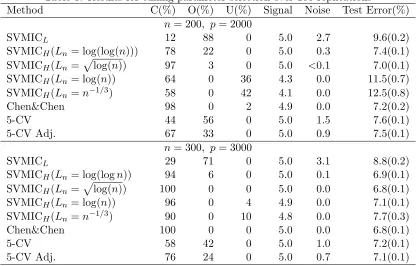
We consider p= 2000 and 3000 and n= 10−1p. Once the data is generated, we construct the solution path of SCAD penalized SVM on a fine grid of λ for candidate models with |S| ≤Mn= 50. We then choose the bestλbased on the definition of SVMICH(λ). Similarly as the simulations for model selection, we compare with SVMICL(λ) and the criterion in Chen and Chen (2008). We also implement five-fold cross-validation (denoted by 5-CV) and an adjusted version of five-fold cross-validation version (denoted by 5-CV Adj.). The adjusted 5-CV selects the most parsimonious model with MSE less than one standard error above the regular 5-CV. It is known that the adjusted 5-CV performs better than regular 5-CV in terms of selection consistency. An independent dataset with sample size 10000 is generated to evaluate the test error. This procedure is repeated for 100 replications to study the variations of the results.
Table 3 summarizes the tuning parameter selection results. It can be seen that the tuning parameter selected by SVMICLoften leads to seriously overfitted models. As the sample size increases, SVMICH with all choices ofLn have a much higher chance to identify the correct model than SVMICL. The tuning parameter selected by SVMICH with Ln =
p
Table 2: Simulation results for Model 2 over 200 replications
Method C(%) O(%) U(%) Signal Noise Test Error(%) n= 200, p= 2000
SVMICL 3.0 96.0 1.0 3.8 5.2 19.2(0.2) SVMICH(Ln= log(log(n))) 31.0 31.5 37.5 3.3 0.5 17.2(0.2) SVMICH(Ln=plog(n)) 25.0 2.5 72.5 3.0 0.1 18.0(0.2) SVMICH(Ln= log(n)) 0.0 0.0 100.0 1.9 0.0 22.1(0.2) SVMICH(Ln=n−1/3) 0.0 0.0 100.0 1.9 0.0 22.1(0.2) Chen&Chen 1.0 0.0 99.0 2.2 0.0 20.4(0.2)
n= 300, p= 3000
SVMICL 6.5 93.5 0.0 4.0 7.4 18.0(0.2)
SVMICH(Ln= log(log(n))) 65.0 23.0 12.0 3.8 0.3 15.0(0.1) SVMICH(Ln=
p
log(n)) 70.5 4.0 25.5 3.7 <0.1 15.3(0.1) SVMICH(Ln= log(n)) 0.0 0.0 100.0 2.0 0.0 21.0(0.1) SVMICH(Ln=n−1/3) 0.0 0.0 100.0 2.0 0.0 21.5(0.2) Chen&Chen 33.5 0.5 66.0 3.1 <0.1 17.3(0.2)
n= 400, p= 4000
SVMICL 9.0 91.0 0.0 4.0 6.9 17.2(0.2) SVMICH(Ln= log(logn)) 82.0 16.5 1.5 4.0 0.2 14.5(0.1) SVMICH(Ln=
p
log(n)) 89.0 2.5 8.5 3.9 <0.1 14.5(0.1) SVMICH(Ln= log(n)) 0.0 0.0 100.0 2.2 0.0 20.1(0.1) SVMICH(Ln=n−1/3) 0.0 0.0 100.0 2.1 0.0 20.8(0.1) Chen&Chen 74.0 0.5 25.5 3.7 <0.1 15.2(0.1)
performances of five-fold cross-validation and its adjusted version are slightly worse than those of SVMICH with Ln fixed at log(log(n)) and plog(n). Notice that the computation burden of selecting tuning parameter via information criterion is much lower than cross-validation. This makes our proposed information criteria desirable especially in the case with very largep.
5. Real data examples
5.1 MAQC-II breast cancer data
In this section we consider a real-world example from the breast cancer dataset which is part of the MicroArray Quality Control (MAQC)-II project. The preprocessed data can be downloaded from GEO databases with accession number GSE20194. There are 278 patient samples in the data and each is described by 22283 genes. Among the 278 samples, 164 patients have positive estrogen receptor (ER) status and 114 have negative ER status. Our goal is to predict the biological endpoint labeled by ER status and pick up the relevant genes.
Table 3: Results for tuning parameter selection over 100 replications
Method C(%) O(%) U(%) Signal Noise Test Error(%) n= 200, p= 2000
SVMICL 12 88 0 5.0 2.7 9.6(0.2)
SVMICH(Ln= log(log(n))) 78 22 0 5.0 0.3 7.4(0.1) SVMICH(Ln=plog(n)) 97 3 0 5.0 <0.1 7.0(0.1) SVMICH(Ln= log(n)) 64 0 36 4.3 0.0 11.5(0.7) SVMICH(Ln=n−1/3) 58 0 42 4.1 0.0 12.5(0.8)
Chen&Chen 98 0 2 4.9 0.0 7.2(0.2)
5-CV 44 56 0 5.0 1.5 7.6(0.1)
5-CV Adj. 67 33 0 5.0 0.9 7.5(0.1)
n= 300, p= 3000
SVMICL 29 71 0 5.0 3.1 8.8(0.2)
SVMICH(Ln= log(logn)) 94 6 0 5.0 0.1 6.9(0.1) SVMICH(Ln=
p
log(n)) 100 0 0 5.0 0.0 6.8(0.1) SVMICH(Ln= log(n)) 96 0 4 4.9 0.0 7.1(0.1) SVMICH(Ln=n−1/3) 90 0 10 4.8 0.0 7.7(0.3) Chen&Chen 100 0 0 5.0 0.0 6.8(0.1)
5-CV 58 42 0 5.0 1.0 7.2(0.1)
5-CV Adj. 76 24 0 5.0 0.7 7.1(0.1)
standardized before fitting the classifier. To reduce the computation burden, only 3000 genes with largest absolute values of the two samplet-statistics are used. Such simplification has been considered in Cai and Liu (2011). Though only 3000 genes are used, the classification result is satisfactory. We implement the SCAD penalized SVM to construct the solution path and set the range of λ as {2−15,2−14, . . . ,23}. The models on the solution path are selected by SVMICL (equivalent toLn= 1), SVMICH withLn at log(log(n)),
p
log(n) and log(n), the criterion adapted from Chen and Chen (2008), five-fold cross-validations and its adjusted version. This procedure is repeated for 200 replications. The corresponding standard errors are summarized in parentheses. Notice that the 3000 genes with the largest absolute values oft-statistics are pre-selected only using the training data to avoid overfitting so they may be different across the 200 random partitions of the data.
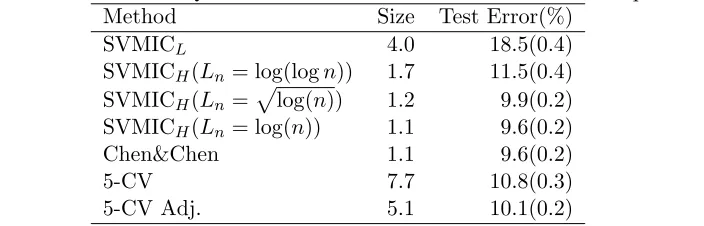
Table 4 summarizes the averages and standard errors for MAQC-II breast cancer data. The criterion SVMICH(λ) performs uniformly better than SVMICL(λ) regardless of the choice of Ln. It can be easily seen that SVMICL(λ) leads to overfitted models in this dataset and has a significant higher misclassification rate. This is in accordance with the theoretical findings in Section 3 that SVMICL can be too liberal when the sample size is not comparable to the number of features, while SVMICH is a consistent model selection criterion. For this dataset, SVMICH with Ln at
p
Figure 1: Test error for MAQC-II breast cancer datasets over 200 random partitions
0.1 0.2 0.3
Ln=1 Ln=log(log(n)) Ln= log(n) Ln=log(n) Chen&Chen 5−CV 5−CV Adj.
T
est Error
stable method than validations across the partitions of the data. Furthermore, cross-validation based on data resampling is more computationally intensive and this discrepancy is expected to increase dramatically if we take all the genes into consideration, which makes the cross-validation less feasible than information criterion method.
Table 4: Results for MAQC-II breast cancer datasets over 200 random partitions Method Size Test Error(%)
SVMICL 4.0 18.5(0.4)
SVMICH(Ln= log(logn)) 1.7 11.5(0.4) SVMICH(Ln=plog(n)) 1.2 9.9(0.2) SVMICH(Ln= log(n)) 1.1 9.6(0.2) Chen&Chen 1.1 9.6(0.2)
5-CV 7.7 10.8(0.3)
5-CV Adj. 5.1 10.1(0.2)
6. Discussion
selection consistency and the ability of selecting tuning parameter when the number of features is much larger than the sample size.
There are several issues yet to be investigated. In this paper we assume that the size of the true model is fixed and the smallest signal does not diminish to zero as the sample size increases. Minimum signal condition has been used in many papers including Fan and Peng (2004) and Fan and Lv (2011). It seems that our condition is stronger than theirs. It is possible to relax this condition. We could possibly assume that q =qn diverges with n such thatqn=O(na1) for some 0≤a1 <1/2. Then we can allow the minimum magnitude
of the nonzero-signal to diminish to zero at an appropriate rate such as min1≤j≤qn|βj∗|> an−(1−a2)/2 for some constanta >0 and 2a
1< a2 ≤1. In general, the condition we impose on min1≤j≤qn|βj∗| is intertwined with the conditions onq and the matrix X, which would be the same for any other high-dimensional regression problem. For a detailed discussion on the beta-min condition in the setting of Lasso regression, we refer to Section 7.4 of B¨uhlmann et al. (2011). Another direction of interest is to extend the information criterion to nonlinear support vector machine. It is well known that the linear support vector machine can be easily extended to nonlinear feature space using the “kernel trick”. Note that it is possible to extend the results in this paper to reproducing kernel Hilbert space with polynomial kernels. For Gaussian radial basis kernels, however, the direct generalization can be problematic as the corresponding reproducing kernel Hilbert space is infinite dimensional. A refined definition of the size of model will be needed in that case and will lead to a more comprehensive study of support vector machine information criterion.
Acknowledgments
Appendix A.
In this appendix we prove the following results from Section 3.2:
Lemma 1 Assuming p is a fixed number and λn= 1/n. Under conditions (A1)-(A4) and (A6)-(A7), we have
Pr(Sb=S∗)→1
as n→ ∞, where Sb= arg minS:|S|≤MSVMICL(S).
Proof. Under regularity conditions, Koo et al. (2008) showed βbS is root-n consistent in
fixed p case for every S ∈ {S :|S| ≤ Mn}. This pointwise result is enough for Lemma 1 since the model space is fixed. The proof is then similar to Lemma 3 and Lemma 4 for divergingpwith the uniform convergence ratep|S|log(p)/nsubstituted by√n−1and thus is omitted here.
Lemma 2 Under conditions (A1)-(A7) andλn= 1/n, we have
sup S:|S|<Mn,S⊃S∗
||βbS−β∗S||=Op( p
|S|log(p)/n).
Proof. Recall that βbS = arg minβ
S{1/n
Pn
i=1(1−YiXTi,SβS)++λn/2||β+S||2}. We will show that for any 0< η <1, there exists a large constant4such that for sufficient largen,
Pr( inf
|S|≤Mn,S⊃S∗||uinf||=4lS(β ∗ S+
p
|S|log(p)/nu)> lS(β∗S))>1−η
where lS(βS) = 1/nPn
i=1(1−YiXTi,SβS)++λn/2||β+S||2. By the convexity of the hinge loss, this implies that with probability 1 −η, we have supS:|S|≤Mn,S⊃S∗||βbS −β∗S|| ≤
4p
|S|log(p)/nand thus Lemma 2 holds.
Notice that we can decompose lS(β∗S+p|S|log(p)/nu)−lS(β∗S) as
lS(β∗S+
p
|S|log(p)/nu)−lS(β∗S)
=1/n n
X
i=1
{(1−YiXTi,S(β∗S+p|S|log(p)/nu))+−(1−YiXTi,Sβ∗S)+}
+λn/2||β∗S++p|S|log(p)/nu+||2−λn/2||β∗S+||2. (10) By the fact ||β∗S++p|S|log(p)/nu+||2− ||β∗+
S ||2 ≤ 4|S|
p
log(p)|S|/n and λn = 1/n, the difference of penalty terms in (10) isn−1|S|o(1). Denote
gi,S(u) =(1−YiXTi,S(β∗S+p|S|log(p)/nu))+−(1−YiXTi,Sβ∗S)+
+p|S|log(p)/nYiXTi,Su1(1−YiXTi,Sβ∗S ≥0)
+E[(1−YiXTi,S(β ∗ S+
p
|S|log(p)/nu))+]−E[(1−YiXTi,Sβ ∗ S)+].
It can easily checked thatE[gi,S(u)] = 0 for{S:|S| ≤Mn, S ⊃S∗}by the definition of β∗S and S(β∗) =0 . Next we consider the difference of hinge loss in (10), which can be further composed as
1/n n
X
i=1
where
An= n
X
i=1
gi,S(u)
and Bn= n X i=1
−p|S|log(p)/nYiXTi,Su1(1−YiXTi,Sβ∗S ≥0)
+E[(1−YiXTi,S(β∗S+
p
|S|log(p)/nu))+]−E[(1−YiXTi,Sβ∗S)+] . The rest of the proof consists of three steps. Step 1 will show
sup |S|≤Mn,S⊃S∗
sup ||u||=4
|An|=|S|op(1).
Step 2 will show inf|S|≤Mn,S⊃S∗inf||u||=4Bn dominates the terms of order|S|op(1) . Step 3 will complete the proof by showing inf|S|≤Mn,S⊃S∗inf||u||=4Bn >0 for sufficient large n and 4.
Step 1: The main tool to prove this uniform rate is the covering number introduced in Van Der Vaart and Wellner (1996). It suffices to show that
Pr( sup |S|≤Mn,S⊃S∗
sup ||u||=4
|S|−1| n
X
i=1
gi,S(u|)> )→0
for any >0. Notice that the hinge loss satisfies Lipschitz condition and by condition (A3) maxi||Xi,S||=Op(
p
|S|log(n)). It can be easily shown that
|S|−1g
i,S(u)≤34|S|−1
p
|S|log(p)/nmax
i ||Xi,S||
and thus sup|S|≤Mn,S⊃S∗sup||u||=4|S|−1gi,S(u) = op(1). By Lemma 2.5 of van de Geer (2000), the ball {u : ||u|| ≤ 4} inR|S|+1 can be covered by N balls with radius δ where N ≤ ((44+δ)/δ)|S|+1. Denote u1, . . . ,uN the centers of the N balls. By the fact that sup|S|≤Mn,S⊃S∗
p
|S|log(p)/nmaxi||Xi,S|| = Op(1), we can take δ = (nC)−1|S| for some large constantC such that
min
1≤k≤N|S|≤Mn,Ssup⊃S∗ sup ||u||=4
|S|−1| n
X
i=1
gi,S(u)− n
X
i=1
gi,S(uk)|
≤ sup |S|≤Mn,S⊃S∗
34n|S|−1p|S|log(p)/nmax
i ||Xi,S||δ ≤ /3 (11)
with probability tending to one. Based on (11), it can be easily shown
Pr( sup |S|≤Mn,S⊃S∗
sup ||u||=4
|S|−1| n
X
i=1
gi,S(u)|> )
≤ X
|S|≤Mn,S⊃S∗ N
X
k=1
Pr(|S|−1| n
X
i=1
and Pn
i=1gi,S(uk) is sum of independent zero-mean random variables. Notice that
(1−YiXTi,S(β∗S+p|S|log(p)/nu))+−(1−YiXTi,Sβ∗S)+
+p|S|log(p)/nYiXTi,Su1(1−YiXTi,Sβ∗S≥0) = 0
when we have |1−YiXTi,Sβ ∗ S|>
p
|S|log(p)/nmaxi||Xi,S||4. Thus we have
n
X
i=1
E[gi,S(uk)]2 =
n
X
i=1
Var(gi,S(uk))
≤ n X i=1 E[(2 p
|S|log(p)/nYiXTi,Suk)21(|1−YiXTi,Sβ∗S| ≤
p
|S|log(p)/nmax
i ||Xi,S||4)]. (12)
By the bounded largest eigenvalue condition in (A3), we have
n
X
i=1
E{[2 p
|S|log(p)/nYiXTi,Suk)]2≤C|S|log(p).
By the bounded conditional density condition (A4), we have
Pr(|1−YiXTi,Sβ ∗ S| ≤
p
|S|log(p)/nmax
i ||Xi,S||4)≤C|S|logn
p
log(p)/n.
Then based on (12) and Cauchy inequality, we have
n
X
i=1
E[gi,S(uk)]2 ≤C|S|2logn(log(p))3/2n−1/2. Then applying Bernstein inequality and condition (A6), we arrive
X
|S|≤Mn,S⊃S∗ N
X
k=1
Pr(|S|−1| n
X
i=1
gi,S(uk)|> /2)
≤exp{Mnlog(p)}exp(N) exp{−C(log(n))−1(log(p))−3/2n1/2} →0 asn→ ∞. This completes the proof of Step 1.
Step 2: First notice that
| n
X
i=1
YiXTi,Su1(1−YiXTi,Sβ∗S ≥0)| ≤(|S|+ 1)1/24 max 0≤j≤p|
n
X
i=1
YiXij,S1(1−YiXTi,Sβ∗S ≥0)|.
(13) Note thatE[YiXij,S1(1−YiXTi,Sβ
∗
S ≥0)] = 0 for 0≤j ≤p by the definition of S(β∗). By Lemma 14.24 of B¨uhlmann et al. (2011), we also have
max 0≤j≤p|
n
X
i=1
By Taylor expansion of hinge loss function at β∗S, we have
n
X
i=1
{E[(1−YiXTi,S(β∗S+p|S|log(p)/nu))+]−E[(1−YiXTi,Sβ∗S)+]}
=0.5|S|log(p)uTH(βS∗ +tp|S|log(p)/nu)u (15)
for some 0< t <1. As shown by Koo et al. (2008), under condition (A1) and (A2), H(β) is element-wise continuous atβ∗S, thus
H(β∗S+tp|S|logp/nu) =H(β∗S) +op(1).
It can be easily shown by (13), (14), (15) and condition (A7), 0.5|S|log(p)uTH(β∗S)u dom-inates other terms in Bn for sufficient large 4. This completes the proof of Step 2.
Step 3: Notice that 0.5|S|log(p)uTH(β∗S)u>0 by condition (A7). Recall that the dif-ference of penalty terms in (10) is n−1|S|o(1). Therefore 0.5|S|logpuTH(β∗S)u dominates all the other terms in (10) for sufficient large nand 4, which completes the proof.
Lemma 3 Under conditions (A1)-(A8) andλn= 1/n, we have
Pr( inf S:S∈Ω+
SVMICH(S)>SVMICH(S∗))→1.
as n→ ∞.
Proof. By definition we have
inf S∈Ω+
SVMICH(S)−SVMICH(S∗)
= inf S∈Ω+
n
X
i=1
(1−YiXTi,SβbS)+−
n
X
i=1
(1−YiXTi,S∗βbS∗)++ (|S| − |S∗|) log(n)Ln .
Similar to the proof of Lemma 2, it can be shown that |Pn
i=1(1−YiXTi,SβbS)+− Pn
i=1(1− YiXTi,S∗βbS∗)+| is dominated by |S|log(p)uTH(β∗S)u with probability tending to one. By conditions (A6)-(A8), we have
| n
X
i=1
(1−YiXTi,SβbS)+−
n
X
i=1
(1−YiXTi,S∗βbS∗)+|<(|S| − |S∗|) log(n)Ln
for sufficient large n. Notice that infS∈Ω+|S| − |S
∗|>0, which completes the proof.
Lemma 4 Under Conditions (A1)-(A8) andλn= 1/n, we have
Pr( inf S:S∈Ω−
SVMICH(S)>SVMICH(S∗))→1.
as n→ ∞.
Proof. ForS∈Ω−, consider the set ˜S with additional signals such that ˜S =S∪S∗. Notice
for S ∈ Ω−. Since |S∗| does not diverge with n, we have |S˜|< 2Mn for sufficiently large n and it can easily seen that Lemma 3 still holds for ˜S with any S ∈Ω−. Therefore with high probability we have SVMICH( ˜S)−SVMICH(S∗)≥0. Thus it suffices to show
Pr( inf S∈Ω−
{SVMICH(S)−SVMICH( ˜S)}>0)→1
asn→ ∞. Notice that
1/n{SVMICH(S)−SVMICH( ˜S)}
=1/n n
X
i=1
(1−YiXTi,SβbS)+−1/n
n
X
i=1
(1−YiXTi,S˜βbS˜)++ 1/n(|S| − |S˜|) log(n)Ln
and by condition (A8) 1/n(|S| − |S˜|) log(n)Ln→0, it suffices to show
inf S∈Ω−
{1/n n
X
i=1
(1−YiXTi,SβbS)+−1/n
n
X
i=1
(1−YiXTi,S˜βbS˜)+} ≥C
for some constantC >0 that does not depend onS.
Recall that βbS = (β0,S, β1,S, . . . , β|S|,S)T ∈ R|S|+1. Denote βbS,S˜ ∈ R|
˜
S|+1 such that the intercept equals toβ0,S, the j-th element equals toβj,S if j ∈S and 0 if j /∈S for all j ∈ S. Denote also˜ δ = minj∈S∗|β∗
j| the smallest signal. Then it can be easily seen that ||βbS,S˜−β∗˜
S||> δ. By Lemma 2 we also have||βbS˜−β ∗
˜
S||< for arbitrary and sufficient largen. Therefore there exists ¯βS˜ =aβbS˜+ (1−a)βbS,S˜ for some 0< a <1 such that
||β¯S˜−β∗S˜||= ∆,
where ∆ is a positive constant such that ∆< c3 where c3 is defined in condition (A7). By the definition of βbS˜ and the convexity of hinge loss function we have
1/n n
X
i=1
(1−YiXTi,S˜β¯S˜)++λn/2||β¯+S˜||2
<a{1/n n
X
i=1
(1−YiXTi,S˜βbS˜)++λn/2||βb
+ ˜ S||2}
+ (1−a){1/n n
X
i=1
(1−YiXTi,SβbS,S˜)++λn/2||βb
+ S,S˜||2} <1/n
n
X
i=1
(1−YiXTi,S˜βbS,S˜)++λn/2||βb
+ S,S˜||2
=1/n n
X
i=1
(1−YiXTi,SβbS)++λn/2||βb
+
S||2. (16)
By λn=n−1 we have
λn/2||β¯+S˜||2−λn/2||βb
+
S||2≤Cλn(||βb
+ ˜
S||2+||βb
+
as n → ∞. Similar to the proof of Lemma 2, under condition (A6) and (A8), it can be shown 1/n n X i=1
(1−YiXTi,S˜βbS˜)+−1/n
n
X
i=1
(1−YiXTi,S˜β∗S˜)+≤1/nC|S˜|log(p)λmax(H(β∗S˜))→0 (18)
asn→ ∞. Notice that
inf S∈Ω−
{1/n n
X
i=1
(1−YiXTi,S˜β¯S˜)+−1/n n
X
i=1
(1−YiXTi,S˜β∗S˜)+} ≥1/n
n
inf S∈Ω−
nE[(1−YiXTi,S˜β¯S˜)+−(1−YiXTi,S˜β ∗
˜ S)+]
− sup S∈Ω−
{| n
X
i=1
(1−YiXTi,S˜β¯S˜)+− n
X
i=1
(1−YiXTi,S˜β∗S˜)+−nE[(1−YiXTi,S˜β¯S˜)+−(1−YiXTi,S˜β∗S˜)+]|}
o
.
Similar to the proof of Lemma 2, it can be shown
sup S∈Ω−
{| n
X
i=1
(1−YiXTi,S˜β¯S˜)+− n
X
i=1
(1−YiXTi,S˜βS∗˜)+−nE[(1−YiXTi,S˜β¯S˜)+−(1−YiXTi,S˜β∗S˜)+]|}
=Op(| n
X
i=1
YiXTi,S˜( ¯βS˜−β∗S˜)1(1−YiXTi,Sβ∗S˜ ≥0)|) =Op(
q
n|S˜|log(p)). (19)
By Taylor expansion of hinge loss function, we have
E[(1−YiXTi,S˜β¯S˜)+−(1−YiXTi,S˜βS∗˜)+]≥0.5λmin(H( ˜β ∗
˜
S))∆2 >0, (20) where ˜β∗S˜ lies in the set defined in condition (A7). By (16)-(20), we have
inf S∈Ω−
{1/n n
X
i=1
(1−YiXTi,SβbS)+−1/n
n
X
i=1
(1−YiXTi,S˜βbS˜)+} ≥0.5λmin(H(β∗˜
S))∆ 2 >0
for sufficient large n, which completes the proof.
Theorem 5 Under conditions (A1)-(A8) andλn= 1/n, we have
Pr( ˆS =S∗)→1.
as n, p→ ∞, where Sb= arg minS:|S|≤MnSVMICH(S).
Proof. The proof can be easily checked by combing the results from Lemma 3 and Lemma 4 and thus is omitted here.
References
Natalia Becker, Grischa Toedt, Peter Lichter, and Axel Benner. Elastic scad as a novel penalization method for svm classification tasks in high-dimensional data. BMC bioin-formatics, 12(1):138, 2011.
Paul S Bradley and Olvi L Mangasarian. Feature selection via concave minimization and support vector machines. InICML, volume 98, pages 82–90, 1998.
Peter Lukas B¨uhlmann, Sara A van de Geer, and Sara Van de Geer. Statistics for high-dimensional data. Springer, 2011.
Tony Cai and Weidong Liu. A direct estimation approach to sparse linear discriminant analysis. Journal of the American Statistical Association, 106(496), 2011.
Jiahua Chen and Zehua Chen. Extended bayesian information criteria for model selection with large model spaces. Biometrika, 95(3):759–771, 2008.
Gerda Claeskens, Christophe Croux, and Johan Van Kerckhoven. An information criterion for variable selection in support vector machines. The Journal of Machine Learning Research, 9:541–558, 2008.
Jianqing Fan and Yingying Fan. High dimensional classification using features annealed independence rules. Annals of statistics, 36(6):2605, 2008.
Jianqing Fan and Runze Li. Variable selection via nonconcave penalized likelihood and its oracle properties. Journal of the American Statistical Association, 96(456):1348–1360, 2001.
Jianqing Fan and Jinchi Lv. Non-concave penalized likelihood with np-dimensionality.IEEE Transactions on Information Theory, 57:5467–5484, 2011.
Jianqing Fan and Heng Peng. On non-concave penalized likelihood with diverging number of parameters. The Annals of Statistics, 32:928–961, 2004.
Yingying Fan and Cheng Yong Tang. Tuning parameter selection in high dimensional pe-nalized likelihood. Journal of the Royal Statistical Society: Series B (Statistical Method-ology), 75(3):531–552, 2013.
Isabelle Guyon and Andr´e Elisseeff. An introduction to variable and feature selection. The Journal of Machine Learning Research, 3:1157–1182, 2003.
Isabelle Guyon, Jason Weston, Stephen Barnhill, and Vladimir Vapnik. Gene selection for cancer classification using support vector machines. Machine learning, 46(1-3):389–422, 2002.
Trevor. Hastie, Robert. Tibshirani, and J Jerome H Friedman. The elements of statistical learning, volume 1. Springer New York, 2001.
Shuichi Kawano. Selection of tuning parameters in bridge regression models via bayesian information criterion. Statistical Papers, pages 1–17, 2012.
Ja-Yong Koo, Yoonkyung Lee, Yuwon Kim, and Changyi Park. A bahadur representation of the linear support vector machine. The Journal of Machine Learning Research, 9: 1343–1368, 2008.
Eun Ryung Lee, Hohsuk Noh, and Byeong U Park. Model selection via bayesian information criterion for quantile regression models. Journal of the American Statistical Association, 109(505):216–229, 2014.
Rahul Mazumder, Jerome H Friedman, and Trevor Hastie. Sparsenet: Coordinate descent with nonconvex penalties. Journal of the American Statistical Association, 106(495), 2011.
Gideon Schwarz. Estimating the dimension of a model. The annals of statistics, 6(2): 461–464, 1978.
Jun Shao. An asymptotic theory for linear model selection. Statistica Sinica, 7(2):221–242, 1997.
Peide Shi and Chih-Ling Tsai. Regression model selectiona residual likelihood approach.
Journal of the Royal Statistical Society: Series B (Statistical Methodology), 64(2):237– 252, 2002.
Sara van de Geer. Empirical processes in m-estimation. cambridge series in statistical and probabilistic mathematics, 2000.
Aad W Van Der Vaart and Jon A Wellner. Weak Convergence. Springer, 1996.
Grace Wahba et al. Support vector machines, reproducing kernel hilbert spaces and the randomized gacv. Advances in Kernel Methods-Support Vector Learning, 6:69–87, 1999.
Hansheng Wang, Runze Li, and Chih-Ling Tsai. Tuning parameter selectors for the smoothly clipped absolute deviation method. Biometrika, 94(3):553–568, 2007.
Hansheng Wang, Bo Li, and Chenlei Leng. Shrinkage tuning parameter selection with a diverging number of parameters. Journal of the Royal Statistical Society: Series B (Statistical Methodology), 71(3):671–683, 2009.
Lan Wang, Yichao Wu, and Runze Li. Quantile regression for analyzing heterogeneity in ultra-high dimension. Journal of the American Statistical Association, 107(497):214–222, 2012.
Li Wang, Ji Zhu, and Hui Zou. The doubly regularized support vector machine. Statistica Sinica, 16(2):589, 2006.
Jason Weston, Sayan Mukherjee, Olivier Chapelle, Massimiliano Pontil, Tomaso Poggio, and Vladimir Vapnik. Feature selection for svms. In NIPS, volume 12, pages 668–674, 2000.
Ming Yuan. High dimensional inverse covariance matrix estimation via linear programming.
The Journal of Machine Learning Research, 99:2261–2286, 2010.
Cun-Hui Zhang. Nearly unbiased variable selection under minimax concave penalty. The Annals of Statistics, 38(2):894–942, 2010.
Cun-Hui Zhang and Jian Huang. The sparsity and bias of the lasso selection in high-dimensional linear regression. The Annals of Statistics, 36(4):1567–1594, 2008.
Hao Helen Zhang, Jeongyoun Ahn, Xiaodong Lin, and Cheolwoo Park. Gene selection using support vector machines with non-convex penalty. Bioinformatics, 22(1):88–95, 2006.
Xiang Zhang, Yichao Wu, Lan Wang, and Runze Li. Variable selection for support vector machines in moderately high dimensions. Journal of the Royal Statistical Society: Series B (Statistical Methodology), 2014.
Ji Zhu, Saharon Rosset, Trevor Hastie, and Rob Tibshirani. 1-norm support vector ma-chines. Advances in neural information processing systems, 16(1):49–56, 2004.
Hui Zou and Runze Li. One-step sparse estimates in nonconcave penalized likelihood models.
Annals of statistics, 36(4):1509, 2008.