Trend Filtering on Graphs

(1)

Trend Filtering on Graphs

Yu-Xiang Wang1,2 [email protected]

James Sharpnack3 [email protected]

Alexander J. Smola1,4 _ALEX_@_SMOLA_._ORG

Ryan J. Tibshirani1,2 [email protected]

1_{Machine Learning Department, Carnegie Mellon University, Pittsburgh, PA 15213}

2_{Department of Statistics, Carnegie Mellon University, Pittsburgh, PA 15213}

3_{Mathematics Department, University of California at San Diego, La Jolla, CA 10280}

4_{Marianas Labs, Pittsburgh, PA 15213}

Editor:Andreas Krause

Abstract

We introduce a family of adaptive estimators on graphs, based on penalizing the`1norm of discrete

graph differences. This generalizes the idea of trend filtering (Kim et al., 2009; Tibshirani, 2014), used for univariate nonparametric regression, to graphs. Analogous to the univariate case, graph trend filtering exhibits a level of local adaptivity unmatched by the usual`2-based graph smoothers.

It is also defined by a convex minimization problem that is readily solved (e.g., by fast ADMM or Newton algorithms). We demonstrate the merits of graph trend filtering through both examples and theory.

Keywords:trend filtering, graph smoothing, total variation denoising, fused lasso, local adaptivity

1. Introduction

Nonparametric regression has a rich history in statistics, carrying well over 50 years of associated literature. The goal of this paper is to port a successful idea in univariate nonparametric regression, trend filtering (Steidl et al., 2006; Kim et al., 2009; Tibshirani, 2014; Wang et al., 2014), to the setting of estimation on graphs. The proposed estimator, graph trend filtering, shares three key properties of trend filtering in the univariate setting.

1. Local adaptivity:graph trend filtering can adapt to inhomogeneity in the level of smoothness of an observed signal across nodes. This stands in contrast to the usual`2-based methods,

e.g., Laplacian regularization (Smola and Kondor, 2003), which enforce smoothness globally with a much heavier hand, and tends to yield estimates that are either smooth or else wiggly throughout.

2. Computational efficiency: graph trend filtering is defined by a regularized least squares problem, in which the penalty term is nonsmooth, but convex and structured enough to permit efficient large-scale computation.

3. Analysis regularization:the graph trend filtering problem directly penalizes (possibly higher order) differences in the fitted signal across nodes. Therefore graph trend filtering falls into what is called theanalysisframework for defining estimators. Alternatively, in thesynthesis

(2)

observed signal over this basis; e.g., Shuman et al. (2013) survey a number of such approaches using wavelets; likewise, kernel methods regularize in terms of the eigenfunctions of the graph Laplacian (Kondor and Lafferty, 2002). An advantage of analysis regularization is that it easily yields complex extensions of the basic estimator by mixing penalties.

As a motivating example, consider a denoising problem on 402 census tracts of Allegheny County, PA, arranged into a graph with 402 vertices and 2382 edges obtained by connecting spa-tially adjacent tracts. To illustrate the adaptive property of graph trend filtering we generated an artificial signal with inhomogeneous smoothness across the nodes, and two sharp peaks near the center of the graph, as can be seen in the top left panel of Figure 1. (The signal was formed using a mixture of five Gaussians, in the underlying spatial coordinates.) We drew noisy observations around this signal, shown in the top right panel of the figure, and we fit graph trend filtering, graph Laplacian smoothing, and wavelet smoothing to these observations. Graph trend filtering is to be defined in Section 2 (here we usedk= 2, quadratic order); the latter two, recall, are defined by the optimization problems

min

β∈_Rn ky−βk 2

2+λβ>Lβ (Laplacian smoothing),

min

θ∈Rn 1

2ky−W θk

2

2+λkθk1 (wavelet smoothing),

wherey∈_Rn_{the vector of observations measured over the}_n_{= 402}_{nodes in the graph,}_L_∈

Rn×n

is the graph Laplacian matrix, and W ∈ _Rn×n _{is a wavelet basis built over the graph. The} wavelet smoothing problem displayed above is really an oversimplified representation of the class of wavelets methods, since it only encapsulates estimators that employ an orthogonal wavelet ba-sis W (and soft-threshold the wavelet coefficients). For the present experiment, we constructed W according to the spanning tree wavelet design of Sharpnack et al. (2013a); we found this con-struction performed best among the graph wavelet designs we considered for the data at hand. For completeness, the results from alternative wavelet designs are given in the Appendix.

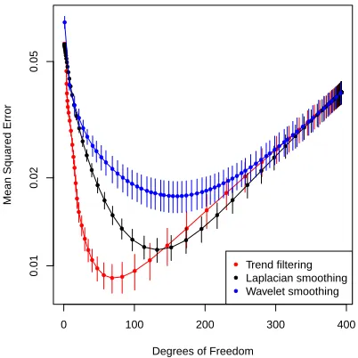
Graph trend filtering, Laplacian smoothing, and wavelet smoothing each have their own regu-larization parametersλ, and these parameters are not generally on the same scale. Therefore, in our comparisons we use effective degrees of freedom (df) as a common measure for the complexities of the fitted models. The top right panel of Figure 1 shows the graph trend filtering estimate with 68 df. We see that it adaptively fits the sharp peaks in the center of the graph, and smooths out the sur-rounding regions appropriately. The graph Laplacian estimate with 68 df (bottom left), substantially oversmooths the high peaks in the center, while at 132 df (bottom middle), it begins to detect the high peaks in the center, but undersmooths neighboring regions. Wavelet smoothing performs quite poorly across all df values—it appears to be most affected by the level of noise in the observations. As a more quantitative assessment, Figure 2 shows the mean squared errors between the es-timates and the true underlying signal. The differences in performance here are analogous to the univariate case, when comparing trend filtering to smoothing splines (Tibshirani, 2014). At smaller df values, Laplacian smoothing, due to its global considerations, fails to adapt to local differences across nodes. Trend filtering performs much better at low df values, and yet it matches Laplacian smoothing when both are sufficiently complex, i.e., in the overfitting regime. This demonstrates that the local flexibility of trend filtering estimates is a key attribute.

(3)

True signal Noisy observations Graph trend filtering, 68 df ● ● ● ● ● ● ● ● ● ● ● ● ● ● ● ● ● ● ● ● 0.056 0.111 0.167 0.223 0.278 0.334 0.389 0.445 0.501 0.556 0.612 0.667 0.723 0.779 0.834 0.89 0.945 1.001 1.057 1.112

Laplacian smoothing, 68 df Laplacian smoothing, 132 df Wavelet smoothing, 160 df

Figure 1: Color maps for the Allegheny County example.

0 100 200 300 400

0.01

0.02

0.05

Degrees of Freedom

Mean Squared Error

● ● ● ● ● ● ● ● ● ● ● ● ● ● ● ● ● ● ● ● ● ● ● ● ● ● ● ● ● ● ● ● ● ● ● ● ● ● ● ● ● ● ● ● ● ● ● ● ● ● ● ● ● ● ● ● ● ● ● ● ● ● ● ● ● ● ● ● ● ● ● ● ● ● ● ● ● ● ● ● ● ● ● ● ● ● ● ● ● ● ● ● ● ● ● ● ● ● ● ● ● ● ● ● ● ● ● ● ● ● ● ● ● ● ● ● ● ● ● ● ● ● ● ● ● ● ● ● ● ● ● ● ● ● ● ● ● ● ● ● ● ● ● ● ● ● ● ● ● ● ● ● ● ● ● ● ● ● ● ● ● ● ● ● ● ● ● ● ● ● ● ● ● ● ● ● ● ● ● ● ● ● ● ● ● ● ● ● ● ● ● ● ● ● ● ● ● ● ● ● ● ● ● ● ● ● ● ● ● ● ● ● ● ● ● ● ● ● ● ● ● ● ● ● ● ● ● ● ● ● ● ● ● ● ● ● ● ● ● ● ● ● ● ● ● ● ● ● ● ● ● ● ● ● ● ● ● ● ● ● ● ● ● ● ● Trend filtering Laplacian smoothing Wavelet smoothing

(4)

trend filtering estimator. Section 4 examines computational approaches, and Section 5 looks at a number of both real and simulated data examples. Section 6 presents asymptotic error bounds for graph trend filtering. Section 7 concludes with a discussion. As for notation, we writeXAto extract the rows of a matrixX ∈_Rm×n_{that correspond to a subset}_A_{⊆ {}₁_{, . . . m}_}_{, and}_X

−Ato extract the complementary rows. We use a similar convention for vectors:xAandx−Adenote the components of a vectorx∈_Rm_{that correspond to the set}_A_{and its complement, respectively. We write}_row(_X₎ andnull(X) for the row and null spaces ofX, respectively, and X†for the pseudoinverse of X, withX†= (X>X)†X>whenXis rectangular.

2. Trend Filtering on Graphs

In this section, we motivate and formally define graph trend filtering.

2.1 Review: Univariate Trend Filtering

We begin by reviewing trend filtering in the univariate setting, where discrete difference operators play a central role. Suppose that we observe y = (y1, . . . yn) ∈ Rn across input locations x =

(x1, . . . xn) ∈ Rn; for simplicity, suppose that the inputs are evenly spaced, say, x = (1, . . . n).

Given an integerk≥0, thekth order trend filtering estimateβˆ= ( ˆβ1, . . .βˆn)is defined as

ˆ

β= argmin

β∈_Rn

1

2ky−βk

2

2+λkD(k+1)βk1, (1)

whereλ≥ 0is a tuning parameter, andD(k+1)is the discrete difference operator of order k+ 1. Whenk= 0, problem (1) employs the first difference operator,

D(1)=



   

−1 1 0 . . . 0

0 −1 1 . . . 0

..

. . .. ...

0 0 . . . −1 1



   

. (2)

ThereforekD(1)βk₁=Pn−1

i=1 |βi+1−βi|, and the 0th order trend filtering estimate in (1) reduces to the 1-dimensional fused lasso estimator (Tibshirani et al., 2005), also called 1-dimensional total variation denoising (Rudin et al., 1992). Fork≥1the operatorD(k+1)is defined recursively by

D(k+1)=D(1)D(k), (3)

withD(1)above denoting the(n−k−1)×(n−k)version of the first difference operator in (2). In words,D(k+1)_{is given by taking first differences of}_{kth differences. The interpretation is hence that}

problem (1) penalizes the changes in thekth discrete differences of the fitted trend. The estimated componentsβˆ1, . . .βˆnexhibit the form of akth order piecewise polynomial function, evaluated over the input locationsx1, . . . xn. This can be formally verified (Tibshirani, 2014; Wang et al., 2014) by examining a continuous-time analog of (1).

2.2 Trend Filtering over Graphs

(5)

definition in (1), we define thekth ordergraph trend filtering(GTF) estimateβˆ= ( ˆβ1, . . .βˆn)by

ˆ

β= argmin

β∈_Rn

1

2ky−βk

2

2+λk∆(k+1)βk1. (4)

In broad terms, this problem (like univariate trend filtering) is a type of generalized lasso problem (Tibshirani and Taylor, 2011), in which the penalty matrix∆(k+1)is a suitably definedgraph differ-ence operator, of orderk+ 1. In fact, the novelty in our proposal lies entirely within the definition of this operator.

When k = 0, we define first order graph difference operator∆(1) in such a way it yields the graph-equivalent of a penalty on local differences:

k∆(1)βk₁= X

(i,j)∈E

|βi−βj|.

so that the penalty term in (4) sums the absolute differences across connected nodes inG. To achieve this, we let∆(1) ∈ {−1,0,1}m×nbe the oriented incidence matrix of the graphG, containing one row for each edge in the graph; specifically, ife`= (i, j), then∆(1)has`th row

∆(1)_` = (0, . . .−1 ↑

i , . . .1

↑

j

, . . .0), (5)

where the orientations of signs are arbitrary. Like trend filtering in the 1d setting, the 0th order graph trend filtering estimate coincides with the fused lasso (total variation regularized) estimate overG (Hoefling, 2010; Tibshirani and Taylor, 2011; Sharpnack et al., 2012).

Fork≥1, we use a recursion to define the higher order graph difference operators, in a manner similar to the univariate case. The recursion alternates in multiplying by the first difference operator ∆(1)_{and its transpose (taking into account that this matrix not square):}

∆(k+1) =

(

(∆(1))>∆(k)=Lk+12 for oddk

∆(1)∆(k)=DLk2 for evenk.

(6)

Above, we abbreviated the oriented incidence matrix∆(1) byDofG, and exploited the fact that L=D>Dis one representation for the graph Laplacian matrix. Note that∆(k+1) ∈_Rn×n_{for odd} k, and∆(k+1) _∈

Rm×nfor evenk.

An important point is that our defined graph difference operators (5), (6) reduce to the univariate ones (2), (3) in the case of a chain graph (in which V = {1, . . . n} andE = {(i, i+ 1) : i = 1, . . . n−1}), modulo boundary terms. That is, whenkis even, if one removes the firstk/2rows and lastk/2rows of∆(k+1) for the chain graph, then one recoversD(k+1); whenkis odd, if one removes the first and last(k+ 1)/2rows of∆(k+1)for the chain graph, then one recoversD(k+1). Further intuition for our graph difference operators is given next.

2.3 Piecewise Polynomials over Graphs

(6)

the components ofβ(Tibshirani, 2014; Wang et al., 2014). Since the components ofβcorrespond to (real-valued) input locationsx = (x1, . . . xn), the interpretation of a piecewise polynomial here is unambiguous. But for a graph, one might ask: does sparsity of∆(k+1)βmean that the components ofβ are piecewise polynomial? And what does the latter even mean, as the components ofβ are defined over the nodes? To address these questions, we intuitivelydefinea piecewise polynomial over a graph, and show that it implies sparsity under our constructed graph difference operators.

• Piecewise constant (k = 0): we say that a signalβ is piecewise constant over a graphGif many of the differencesβi−βjare zero across edges(i, j)∈EinG. Note that this is exactly the property associated with sparsity of∆(1)β, since∆(1)=D, the oriented incidence matrix ofG.

• Piecewise linear (k= 1):we say that a signalβhas a piecewise linear structure overGifβ satisfies

βi−

1 ni

X

(i,j)∈E

βj = 0,

for many nodes i ∈ V, where ni is the number of nodes adjacent to i. In words, we are requiring that the signal components can be linearly interpolated from its neighboring values at many nodes in the graph. This is quite a natural notion of (piecewise) linearity: requiring thatβibe equal to the average of its neighboring values would enforce linearity at βi under an appropriate embedding of the points in Euclidean space. Again, this is precisely the same as requiring∆(2)β to be sparse, since∆(2) =L, the graph Laplacian.

• Piecewise polynomial (k≥2):We say thatβhas a piecewise quadratic structure overGif the first differencesαi−αj of the second differencesα= ∆(2)βare mostly zero, over edges

(i, j) ∈ E. Likewise, β has a piecewise cubic structure over G if the second differences αi−_n1

i

P

(i,j)∈Eαj of the second differencesα = ∆(2)βare mostly zero, over nodesi∈V. This argument extends, alternating between leading first and second differences for even and oddk. Sparsity of∆(k+1)β in either case exactly corresponds to many of these differences being zero, by construction.

In Figure 3, we illustrate the graph trend filtering estimator on a 2d grid graph of dimension 20×20, i.e., a grid graph with 400 nodes and 740 edges. For each of the casesk = 0,1,2, we generated synthetic measurements over the grid, and computed a GTF estimate of the corresponding order. We chose the 2d grid setting so that the piecewise polynomial nature of GTF estimates could be visualized. Below each plot, the utilized graph trend filtering penalty is displayed in more explicit detail.

2.4 `1 versus`2Regularization

It is instructive to compare the graph trend filtering estimator, as defined in (4), (5), (6) to Laplacian smoothing (Smola and Kondor, 2003). Standard Laplacian smoothing uses the same least squares loss as in (4), but replaces the penalty term withβ>Lβ. A natural generalization would be to allow for a power of the Laplacian matrixL, and definekth order graph Laplacian smoothing according to

ˆ

β = argmin

β∈Rn

(7)

GTF withk= 0 GTF withk= 1 ● ● ● ● ● ● ● ● ● ● ● ● ● ● ● ● ● ● ● ● ● ● ● ● ● ● ● ● ● ● ● ● ● ● ● ● ● ● ● ● ● ● ● ● ● ● ● ● ● ● ● ● ● ● ● ● ● ● ● ● ● ● ● ● ● ● ● ● ● ● ● ● ● ● ● ● ● ● ● ● ● ● ● ● ● ● ● ● ● ● ● ● ● ● ● ● ● ● ● ● ● ● ● ● ● ● ● ● ● ● ● ● ● ● ● ● ● ● ● ● ● ● ● ● ● ● ● ● ● ● ● ● ● ● ● ● ● ● ● ● ● ● ● ● ● ● ● ● ● ● ● ● ● ● ● ● ● ● ● ● ● ● ● ● ● ● ● ● ● ● ● ● ● ● ● ● ● ● ● ● ● ● ● ● ● ● ● ● ● ● ● ● ● ● ● ● ● ● ● ● ● ● ● ● ● ● ● ● ● ● ● ● ● ● ● ● ● ● ● ● ● ● ● ● ● ● ● ● ● ● ● ● ● ● ● ● ● ● ● ● ● ● ● ● ● ● ● ● ● ● ● ● ● ● ● ● ● ● ● ● ● ● ● ● ● ● ● ● ● ● ● ● ● ● ● ● ● ● ● ● ● ● ● ● ● ● ● ● ● ● ● ● ● ● ● ● ● ● ● ● ● ● ● ● ● ● ● ● ● ● ● ● ● ● ● ● ● ● ● ● ● ● ● ● ● ● ● ● ● ● ● ● ● ● ● ● ● ● ● ● ● ● ● ● ● ● ● ● ● ● ● ● ● ● ● ● ● ● ● ● ● ● ●● ● ● ● ● ● ● ● ● ● ● ● ● ● ● ● ● ● ● ● ● ● ● ● ● ●● ● ● ● ● ● ● ●● ● ● ● ● ● ● ● ● ● ● ● ● ● ● ● ● ● ● ● ● ● ● ● ● ● ● ● ● ● ● ● ● ● ● ● ● ● ● ● ● ● ● ● ● ● ● ● ● ● ● ● ● ● ● ● ● ● ● ● ● ● ● ● ● ● ● ● ● ● ● ● ● ● ● ● ● ● ● ● ● ● ● ● ● ● ● ● ● ● ● ● ● ● ● ● ● ● ● ● ● ● ● ● ● ● ● ● ● ● ● ● ● ● ● ● ● ● ● ● ● ● ● ● ● ● ● ● ● ● ● ● ● ● ● ● ● ● ● ● ● ● ● ● ● ● ● ● ● ● ● ● ● ● ● ● ● ● ● ● ● ● ● ● ● ● ● ● ● ● ● ● ● ● ● ● ● ● ● ● ● ● ● ● ● ● ● ● ● ● ● ● ● ● ● ● ● ● ● ● ● ● ● ● ● ● ● ● ● ● ● ● ● ● ● ● ● ● ● ● ● ● ● ● ● ● ● ● ● ● ● ● ● ● ● ● ● ● ● ● ● ● ● ● ● ● ● ● ● ● ● ● ● ● ● ● ● ● ● ● ● ● ● ● ● ● ● ● ● ● ● ● ● ● ● ● ● ● ● ● ● ● ● ● ● ● ● ● ● ● ● ● ● ● ● ● ● ● ● ● ● ● ● ● ● ● ● ● ● ● ● ● ● ● ● ● ● ● ● ● ● ● ● ● ● ● ● ● ● ● ● ● ● ● ● ● ● ● ● ● ● ● ● ● ● ● ● ● ● ● ● ● ● ● ● ● ● ● ● ● ● ● ● ● ● ● ● ● ●● ● ● ● ● ●●● ● ● ● ● ● ● ● ●● ● ● ● ●●● ● ● ● ● ● ●● ● ● ● ● Penalty: X

(i,j)∈E

|βi−βj|

n X i=1 ni

βi−

1 ni

X

j:(i,j)∈E βj

GTF withk= 2

● ● ● ● ● ● ● ● ● ● ● ● ● ● ● ● ● ● ● ● ● ● ● ● ● ● ● ● ● ● ● ● ● ● ● ● ● ● ● ● ● ● ● ● ● ● ● ● ● ● ● ● ● ● ● ● ● ● ● ● ● ● ● ● ● ● ● ● ● ● ● ● ● ● ● ● ● ● ● ● ● ● ● ● ● ● ● ● ● ● ● ● ● ● ● ● ● ● ● ● ● ● ● ● ● ● ● ● ● ● ● ● ● ● ● ● ● ● ● ● ● ● ● ● ● ● ● ● ● ● ● ● ● ● ● ● ● ● ● ● ● ● ● ● ● ● ● ● ● ● ● ● ● ● ● ● ● ● ● ● ● ● ● ● ● ● ● ● ● ● ● ● ● ● ● ● ● ● ● ● ● ● ● ● ● ● ● ● ● ● ● ● ● ● ● ● ● ● ● ● ● ● ● ● ● ● ● ● ● ● ● ● ● ● ● ● ● ● ● ● ● ● ● ● ● ● ● ● ● ● ● ● ● ● ● ● ● ● ● ● ● ● ● ● ● ● ● ● ● ● ● ● ● ● ● ● ● ● ● ● ● ● ● ● ● ● ● ● ● ● ● ● ● ● ● ● ● ● ● ● ● ● ● ● ● ● ● ● ● ● ● ● ● ● ● ● ● ● ● ● ● ● ● ● ● ● ● ● ● ● ● ● ● ● ● ● ● ● ● ● ● ● ● ● ● ● ● ● ● ● ● ● ● ● ● ● ● ● ● ● ● ● ● ● ● ● ● ● ● ● ● ● ● ● ●● ● ● ● ● ● ● ● ● ● ● ● ● ● ● ● ● ●● ● ● ● ● ● ● ● ● ● ● ●● ● ● ● ● ● ● ● ●● ● ● ● ● ● X

(i,j)∈E ni

βi−

1 ni

X

`:(i,`)∈E β`

−nj

βj −

1 nj

X

`:(j,`)∈E β`

Figure 3: Graph trend filtering estimates of ordersk = 0,1,2on a 2d grid. The utilized`1 graph

(8)

The above penalty term can be written askL(k+1)/2βk2

2 for oddk, andkDLk/2βk22 for evenk; i.e.,

this penalty is exactlyk∆(k+1)βk2

2for the graph difference operator∆(k+1)defined previously.

As we can see, the critical difference between graph Laplacian smoothing (7) and graph trend filtering (4) lies in the choice of penalty norm:`2in the former, and`1in the latter. The effect of the

`1 penalty is that the GTF program can set many (higher order) graph differences to zero exactly,

and leave others at large nonzero values; i.e., the GTF estimate can simultaneously be smooth in some parts of the graph and wiggly in others. On the other hand, due to the (squared)`2penalty, the

graph Laplacian smoother cannot set any graph differences to zero exactly, and roughly speaking, must choose between making all graph differences small or large. The relevant analogy here is the comparison between the lasso and ridge regression, or univariate trend filtering and smoothing splines (Tibshirani, 2014), and the suggestion is that GTF can adapt to the proper local degree of smoothness, while Laplacian smoothing cannot. This is strongly supported by the examples given throughout this paper.

2.5 Related Work

Some authors from the signal processing community, e.g., Bredies et al. (2010); Setzer et al. (2011), have studied total generalized variation (TGV), a higher order variant of total variation regulariza-tion. Moreover, several discrete versions of these operators have been proposed. They are often similar to the construction that we have. However, the focus of these works is mostly on how well a discrete functional approximates its continuous counterpart. This is quite different from our con-cern, as a signal on a graph (say a social network) may not have any meaningful continuous-space embedding at all. In addition, we are not aware of any study on the statistical properties of these regularizers. In fact, our theoretical analysis in Section 6 may be extended to these methods too.

3. Properties and Extensions

We first study the structure of graph trend filtering estimates, then discuss interpretations and exten-sions.

3.1 Basic Structure and Degrees of Freedom

We describe the basic structure of graph trend filtering estimates and present an unbiased estimate for their degrees of freedom. Let the tuning parameterλbe arbitrary but fixed. By virtue of the`1

penalty in (4), the solutionβˆsatisfiessupp(∆(k+1)βˆ) = Afor some active setA (typicallyAis smaller whenλis larger). Trivially, we can reexpress this as∆(₋k_A+1)βˆ= 0, orβˆ∈null(∆(₋k_A+1)). Therefore, the basic structure of GTF estimates is revealed by analyzing the null space of the sub-operator∆(₋k_A+1).

Lemma 1 Assume without a loss of generality thatGis connected (otherwise the results apply to each connected component ofG). LetD, Lbe the oriented incidence matrix and Laplacian matrix ofG. For evenk, letA ⊆ {1, . . . m}, and letG−A denote the subgraph induced by removing the edges indexed byA(i.e., removing edgese`,`∈A). LetC1, . . . Csbe the connected components of G−A. Then

null(∆(₋k_A+1)) = span{₁}+ (L†)k2span{1C

(9)

where 1 = (1, . . .1) ∈ _Rn_{, and} _1C

1, . . .1Cs ∈ R

n _{are the indicator vectors over connected}

components. For oddk, letA⊆ {1, . . . n}. Then

null(∆(₋k_A+1)) = span{₁}+{(L†)k+12 v:v₋_A= 0}.

The proof of Lemma 1 appears in the Appendix. The lemma is useful for a few reasons. First, as motivated above, it describes the coarse structure of GTF solutions. When k = 0, we can see (as (L†)0/2=I) that βˆwill indeed be piecewise constant over groups of nodesC1, . . . Cs of G. Fork = 2,4, . . ., this structure is smoothed by multiplying such piecewise constant levels by (L†)k/2. Meanwhile, fork = 1,3. . ., the structure of the GTF estimate is based on assigning nonzero values to a subsetAof nodes, and then smoothing through multiplication by(L†)(k+1)/2. Both of these smoothing operations, which depend onL†, have interesting interpretations in terms of to the electrical network perspective for graphs. This is developed in the next subsection.

A second use of Lemma 1 is that it leads to a simple expression for the degrees of freedom, i.e., the effective number of parameters, of the GTF estimateβ. From results on generalized lasso prob-ˆ lems (Tibshirani and Taylor, 2011, 2012), we havedf( ˆβ) =E[nullity(∆(−kA+1))], withA denoting the support of∆(k+1)β, andˆ nullity(X)the dimension of the null space of a matrixX. Applying Lemma 1 then gives the following.

Lemma 2 Assume thatGis connected. Letβˆdenote the GTF estimate at a fixed but arbitrary value ofλ. Under the normal error modely ∼ N(β0, σ2I), the GTF estimateβˆhas degrees of freedom given by

df( ˆβ) =

(

E[max{|A|,1}] oddk,

E[number of connected components of G−A] evenk.

HereA= supp(∆(k+1)βˆ)denotes the active set ofβˆ.

As a result of Lemma 2, we can form simple unbiased estimate for df( ˆβ); for kodd, this is max{|A|,1}, and forkeven, this is the number of connected components ofG−A, whereAis the support of∆(k+1)β. When reporting degrees of freedom for graph trend filtering (as in the exampleˆ in the introduction), we use these unbiased estimates.

3.2 Electrical Network Interpretation

Lemma 1 reveals a mathematical structure for GTF estimatesβ, which satisfyˆ βˆ∈null(∆(₋k_A+1)) for some setA. It is interesting to interpret the results using the electrical network perspective for graphs (Vishnoi, 2012). In this perspective, we imagine replacing each edge in the graph with a resistor of value 1. Ifu ∈ _Rn _{describes how much current is going in at each node in the graph,} thenv=Ludescribes the induced voltage at each node. Provided that1>c= 0, which means that the total accumulation of current in the network is 0, we can solve for the current values from the voltage values:u=L†v.

The odd case in Lemma 1 asserts that

null(∆(₋k_A+1)) = span{₁}+{(L†)k+12 v:v₋_A= 0}.

(10)

vector by a constant amount). Fork = 3, we assign a sparse number of nodes a nonzero voltage, solve for the induced current, and thenrepeat this: we relabel the induced current as input voltages to the nodes, and compute the new induced current. This process is again iterated fork= 5,7, . . ..

The even case in Lemma 1 asserts that

null(∆(₋k_A+1)) = span{₁}+ (L†)k2span{1C

1, . . .1Cs}.

For k = 2, this result says that GTF estimates are given by choosing a partitionC1, . . . Csof the nodes, and assigning a constant input voltage to each element of the partition. We then solve for the induced current (and potentially shift this by an overall constant amount). The process is iterated fork= 4,6, . . .by relabeling the induced current as input voltage.

The comparison between the structure of estimates for k = 2andk = 3is informative: in a sense, the above tells us that 2nd order GTF estimates will besmootherthan 3rd order estimates, as a sparse input voltage vector need not induce a current that is piecewise constant over nodes in the graph. For example, an input voltage vector that has only a few nodes with very large nonzero values will induce a current that is peaked around these nodes, but not piecewise constant.

3.3 Extensions

Several extensions of the proposed graph trend filtering model are possible. Trend filtering over a weighted graph, for example, could be performed by using a properly weighted version of the edge incidence matrix in (5), and carrying forward the same recursion in (6) for the higher order difference operators. As another example, the Gaussian regression loss in (4) could be changed to another suitable likelihood-derived losses in order to accommodate a different data type fory, say, logistic regression loss for binary data, or Poisson regression loss for count data.

In Section 5.2, we explore a modest extension of GTF, where we add a strongly convex prior term to the criterion in (4) to assist in performing graph-based imputation from partially observed data over the nodes. In Section 5.3, we investigate a modification of the proposed regularization scheme, where we add a pure`1 penalty onβin (4), hence forming a sparse variant of GTF. Other

potentially interesting penalty extensions include: mixing graph difference penalties of various or-ders, and tying together several denoising tasks with a group penalty. Extensions such as these are easily built, recall, as a result of the analysis framework used by the GTF program, wherein the esti-mate defined through direct regularization via an analyzing operator, the`1-based graph difference

penaltyk∆(k+1)_β_k 1.

4. Computation

Graph trend filtering is defined by a convex optimization problem (4). In principle this means that, at least for small or moderately sized problems, its solutions can be reliably computed using a variety of standard algorithms. In order to handle larger scale problems, we describe two specialized algorithms that improve on generic procedures by taking advantage of the structure of∆(k+1)_.

4.1 A Fast ADMM Algorithm

(11)

even and oddkare

min

β,z∈Rn 1

2ky−βk

2

2+λkDzk1 s.t. z=L k 2x,

min

β,z∈Rn 1

2ky−βk

2

2+λkzk1 s.t. z=L k+1

2 x,

respectively. Recall that Dis the oriented incidence matrix and L is the graph Laplacian. The augmented Lagrangian is

1

2ky−βk

2

2+λkSzk1+

ρ 2kz−L

q_β₊_u_k2 2−

ρ 2kuk

2 2,

whereS = D orS = I depending on whetherk is even or odd, and likewiseq = k/2orq = (k+ 1)/2. ADMM then proceeds by iteratively minimizing the augmented Lagrangian over β, minimizing overz, and performing a dual update overu. Theβ andzupdates are of the form, for someb,

β←(I+ρL2q)−1b, (8)

z←argmin

x∈_Rn

1

2kb−xk

2 2+

λ

ρkSxk1, (9)

The linear system in (8) is well-conditioned, sparse, and can be solved efficiently using the pre-conditioned conjugate gradient method. This involves only multiplication with Laplacian matrices. For a small enough choices ofρ > 0(the augmented Lagrangian parameter), the system in (8) is diagonally dominant, special Laplacian/SDD solvers can be applied, which run in almost linear time (Spielman and Teng, 2004; Koutis et al., 2011; Kelner et al., 2013).

ForS =I, the update in (9) is simply given by soft-thresholding, and forS =D, it is given by graph TV denoising, i.e., given by solving a graph fused lasso problem. Note that this subproblem has the exact structure of the graph trend filtering problem (4) withk = 0. A direct approach for graph TV denoising is available based on parametric max-flow (Chambolle and Darbon, 2009), and this algorithm is empirically much faster than its worst-case complexity (Boykov and Kolmogorov, 2004). In the special case that the underlying graph is a grid, a promising alternative method em-ploys proximal stacking techniques (Barbero and Sra, 2014).

4.2 A Fast Newton Method

As an alternative to ADMM, a projected Newton-type method (Bertsekas, 1982; Barbero and Sra, 2011) can be used to solve (4) via its dual problem:

ˆ

v= argmin

v∈Rr

ky−(∆(k+1))>vk2

2 s.t. kvk∞≤λ.

The solution of (4) is then given byβˆ=y−(∆(k+1))>v. (For univariate trend filtering, Kim et al.ˆ (2009) adopt a similar strategy, but instead use an interior point method.) The projected Newton method performs updates using a reduced Hessian, so abbreviating ∆ = ∆(k+1), each iteration boils down to

(12)

for some a, b and set of indices I. The linear system in (10) is always sparse, but conditioning becomes an issue askgrows (note that the same problem does not occur in (8) because of the addi-tion of the identity matrixI). We have found empirically that a preconditioned conjugate gradient method works quite well for (10) fork= 1, but struggles for largerk.

4.3 Computation Summary

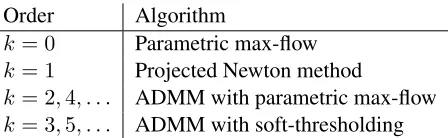
In our experience, the following algorithms work well for the various orderkof graph trend filtering. We remark that ordersk= 0,1,2are of most practical interest (and solutions of polynomial order k≥3are less likely to be sought in practice).1

Order Algorithm

k= 0 Parametric max-flow k= 1 Projected Newton method

k= 2,4, . . . ADMM with parametric max-flow k= 3,5, . . . ADMM with soft-thresholding

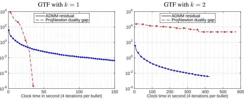
Figure 4 compares performances of the described algorithms on a moderately large simulated example, using a 2d grid graph. We see that whenk= 1, the projected Newton method converges faster than ADMM (superlinear versus at best linear convergence). When k = 2, the story is reversed, as the projected Newton iterations quickly become stagnant, and the ADMM enjoys better convergence.

5. Examples

In this section, we present a variety of examples of running graph trend filtering on real graphs.

5.1 Trend Filtering over the Facebook Graph

In the Introduction, we examined the denoising power of graph trend filtering in a spatial setting. Here we examine the behavior of graph trend filtering on a nonplanar graph: the Facebook graph from the Stanford Network Analysis Project (http://snap.stanford.edu). This is com-posed of 4039 nodes representing Facebook users, and 88,234 edges representing friendships, col-lected from real survey participants; the graph has one connected component, but the observed degree sequence is very mixed, ranging from 1 to 1045 (refer to McAuley and Leskovec (2012) for more details).

We generated synthetic measurements over the Facebook nodes (users) based on three different ground truth models, so that we can precisely evaluate and compare the estimation accuracy of GTF, Laplacian smoothing, and wavelet smoothing. For the latter, we again used the spanning tree wavelet design of Sharpnack et al. (2013a), because it performed among the best of wavelets designs in all data settings considered here. Results from other wavelet designs are presented in

(13)

GTF withk = 1 GTF withk = 2

Clock time in second (4 iterations per bullet)

0 50 100 150

10-6 10-4 10-2 100 102 104

ADMM residual ProjNewton duality gap

Clock time in second (4 iterations per bullet)

0 100 200 300 400 500 600

10-4 10-2 100 102 104 106

ADMM residual ProjNewton duality gap

Figure 4: Convergence plots for projected Newton method and ADMM for solving GTF withk= 1 andk= 2. The algorithms are all run on a 2d grid graph (an512×512image) with 262,144 nodes and 523,264 edges. For projected Newton, we plot the duality gap across iterations; for ADMM, we plot the average of the primal and dual residuals (which also serves as a valid suboptimality bound in the ADMM framework).

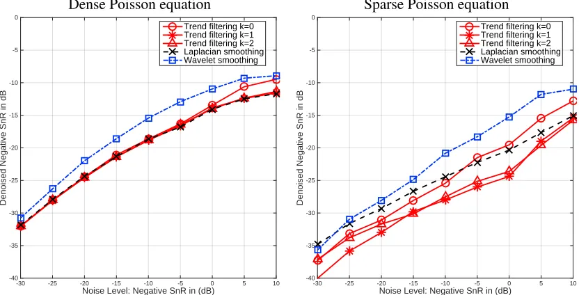
the Appendix. The three ground truth models represent very different scenarios for the underlying signalx, each one favorable to different estimation methods. These are:

1. Dense Poisson equation:we solved the Poisson equationLx=bforx, wherebis arbitrary and dense (its entries were i.i.d. normal draws).

2. Sparse Poisson equation: we solved the Poisson equationLx = bforx, wherebis sparse and has 30 nonzero entries (again i.i.d. normal draws).

3. Inhomogeneous random walk: we ran a set of decaying random walks at different starter nodes in the graph, and recorded inxthe total number of visits at each node. Specifically, we chose 10 nodes as starter nodes, and assigned each starter node a decay probability uniformly at random between 0 and 1 (this is the probability that the walk terminates at each step instead of travelling to a neighboring node). At each starter node, we also sent out a varying number of random walks, chosen uniformly between 0 and 1000.

In each case, the synthetic measurements were formed by adding noise tox. We note that model 1 is designed to be favorable for Laplace smoothing; model 2 is designed to be favorable for GTF; and in the inhomogeneity in model 3 is designed to be challenging for Laplacian smoothing, and favorable for the more adaptive GTF and wavelet methods.

(14)

Dense Poisson equation Sparse Poisson equation

Noise Level: Negative SnR in (dB)

-30 -25 -20 -15 -10 -5 0 5 10

Denoised Negative SnR in dB

-40 -35 -30 -25 -20 -15 -10 -5 0

Trend filtering k=0 Trend filtering k=1 Trend filtering k=2 Laplacian smoothing Wavelet smoothing

-30 -25 -20 -15 -10 -5 0 5 10

-40 -35 -30 -25 -20 -15 -10 -5 0

Inhomogeneous random walk

-30 -25 -20 -15 -10 -5 0 5 10

-40 -35 -30 -25 -20 -15 -10 -5 0

Figure 5: Performance of GTF and others for three generative models on the Facebook graph. The x-axis shows the negative SnR:10 log₁₀(nσ2/kxk2

2), wheren = 4039,xis the underlying signal,

andσ2is the noise variance. Hence the noise level is increasing from left to right. The y-axis shows the denoised negative SnR:10 log₁₀(MSE/kxk2

2), where MSE denotes mean squared error, so the

(15)

5.2 Graph-Based Transductive Learning over UCI Data

Graph trend filtering can used for graph-based transductive learning, as motivated by the work of Talukdar and Crammer (2009); Talukdar and Pereira (2010), who rely on Laplacian regulariza-tion. Consider a semi-supervised learning setting, where we are given only a small number of seed labels over nodes of a graph, and the goal is to impute the labels on the remaining nodes. Write O ⊆ {1, . . . n} for the set of observed nodes, and assume that each observed label falls into {1, . . . K}. Then we can define the modified absorption problem under graph trend filtering regularization (MAD-GTF) by

ˆ

B = argmin

B∈_Rn×K

K X

j=1

X

i∈O

(Yij−Bij)2+λ K X

j=1

k∆(k+1)Bjk1+

K X

j=1

kRj −Bjk22. (11)

The matrixY ∈ Rn×K is an indicator matrix: each observed rowi ∈ O is described byYij = 1 if classj is observed andYij = 0otherwise. The matrixB ∈ Rn×K contains fitted probabilities,

withBij giving the probability that nodeiis of classj. We writeBj for itsjth column, and hence the middle term in the above criterion encourages each set of class probabilities to behave smoothly over the graph. The last term in the above criterion ties the fitted probabilities to some given prior weightsR ∈ _Rn×K_{. In principle}_{could act as a second tuning parameter, but for simplicity we} taketo be small and fixed, with any >0guaranteeing that the criterion in (11) is strictly convex, and thus has a unique solutionBˆ. The entries ofBˆ need not be probabilites in any strict sense, but we can still interpret them as relative probabilities, and imputation can be performed by assigning each unobserved nodei /∈Oa class labeljsuch thatBˆij is largest.

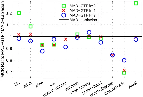
0.7 0.8 0.9 1 1.1 1.2

MCR Ratio: MAD−GTF / MAD−Laplacian

iris _adult _wine car

breast−cancer abalone

wine−qualitypoker−hand

heart−diseaseinternet−ads yeast MAD−GTF k=0

MAD−GTF k=1 MAD−GTF k=2 MAD−Laplacian

Figure 6: Ratio of the misclassification rate of MAD-GTF to MAD-Laplacian, for graph-based imputation, on the 11 most popular UCI classification data sets.

(16)

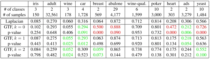
iris adult wine car breast abalone wine-qual. poker heart ads yeast

# of classes 3 2 3 4 2 29 6 10 2 2 10

# of samples 150 32,561 178 1,728 569 4,177 1,599 3,000 303 3,279 1,484 Laplacian 0.085 0.270 0.060 0.316 0.064 0.872 0.712 0.814 0.208 0.306 0.566 GTF,k= 0 0.102 0.293 0.055 0.294 0.500 0.888 0.709 0.801 0.472 0.212 0.726

p-value 0.254 0.648 0.406 0.091 0.000 0.090 0.953 0.732 0.000 0.006 0.000

GTF,k= 1 0.087 0.275 0.055 0.293 0.063 0.874 0.713 0.813 0.175 0.218 0.563 p-value 0.443 0.413 0.025 0.012 0.498 0.699 0.920 0.801 0.134 0.054 0.636 GTF,k= 2 0.084 0.259 0.052 0.309 0.059 0.865 0.738 0.774 0.175 0.244 0.552

p-value 0.798 0.482 0.024 0.523 0.073 0.144 0.479 0.138 0.301 0.212 0.100

Table 1: Misclassification rates of MAD-Laplacian and MAD-GTF for imputation in the UCI data sets. We also compute p-values over the 10 repetitions for each data set (10 draws of nodes to serve as seed labels) via paired t-tests. Cases where MAD-GTF achieves significantly better misclassifica-tion rate, at the 0.1 level, are highlighted ingreen; cases where MAD-GTF achieves a significantly worse miclassification rate, at the 0.1 level, are highlighted inred.

to have heterogeneous smoothness over the graph, then replacing the Laplacian regularizer with the GTF-designed one might lead to better performance. As a broad comparison of the two meth-ods, we ran them on the 11 most popular classification data sets from the UCI Machine Learning repository (http://archive.ics.uci.edu/ml/).2 For each data set, we constructed a5 -nearest-neighbor graph based on the Euclidean distance between provided features, and randomly selected 5 seeds per class to serve as the observed class labels. Then we set = 0.01, used prior weightsRij = 1/K for alliandj, and chose the tuning parameterλover a wide grid of values to represent the best achievable performance by each method, on each experiment. Figure 6 and Table 1 summarize the misclassification rates from imputation using Laplacian and MAD-GTF, averaged over 10 repetitions of the randomly selected seed labels. We see that MAD-GTF withk = 0(basically a graph partition akin to MRF-based graph cut, using an Ising model) does not seem to work as well as the smoother alternatives. Importantly, MAD-GTF with k = 1and k= 2both perform at least as well, and sometimes better, than MAD-Laplacian on each one of the UCI data sets. Recall that these data sets were selected entirely based on their popularity, and not at all on the belief that they might represent favorable scenarios for GTF (i.e., not on the prospect that they might exhibit some heterogeneity in the distribution of class labels over their respective graphs). Therefore, the fact that MAD-GTF nonetheless performs competitively in such a broad range of experiments is convincing evidence for the utility of the GTF regularizer.

5.3 Event Detection with NYC Taxi Trips Data

We illustrate a sparse variant of our proposed regularizers, given by adding a pure`1 penalty to the

coefficients in (4), as in

ˆ

β = argmin

β∈_Rn

1

2ky−βk

2

2+λ1k∆(k+1)βk1+λ2kβk1. (12)

We call thissparse graph trend filtering, now with two tuning parametersλ1, λ2 ≥ 0. Under the

proper tuning, the sparse GTF estimate will be zero at many nodes in the graph, and will otherwise

(17)

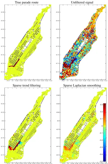
deviate smoothly from zero. This can be useful in situations where the observed signal represents a difference between two smooth processes that are mostly similar, but exhibit (perhaps significant) differences over a few regions of the graph. Here we apply it to the problem of detecting events based on abnormalities in the number of taxi trips at different locations of New York city. This data set was kindly provided by authors of Doraiswamy et al. (2014), who obtained the data from NYC Taxi & Limosine Commission.3 Specifically, we consider the graph to be the road network of Manhattan, which contains 3874 nodes (junctions) and 7070 edges (sections of roads that connect two junctions). For measurements over the nodes, we used the number of taxi pickups and dropoffs over a particular time period of interest: 12:00–2:00 pm on June 26, 2011, corresponding to the Gay Pride parade. As pickups and dropoffs do not generically occur at road junctions, we used interpolation to form counts over the graph nodes. A baseline seasonal average was calculated by considering data from the same time block 12:00–2:00 pm on the same day of the week across the nearest eight weeks. Thus the measurements y were then taken to be the difference between the counts observed during the Gay Pride parade and the seasonal averages.

Note that the nonzero node estimates from sparse GTF applied toy, after proper tuning, mark events of interest, because they convey substantial differences between the observed and expected taxi counts. According to descriptions in the news, we know that the Gay Pride parade was a giant march down at noon from 36th St. and Fifth Ave. all the way to Christopher St. in Greenwich Village, and traffic was blocked over the entire route for two hours (meaning no pickups and dropoffs could occur). We therefore hand-labeled this route as a crude “ground truth” for the event of interest, illustrated in the left panel of Figure 7.

In the bottom two panels of Figure 7, we compare sparse GTF with k = 0(i.e., the sparse graph fused lasso) and a sparse variant of Laplacian smoothing, obtained by replacing the first regularization term in (12) byβ>Lβ. For a qualitative visual comparison, the smoothing parameter λ1was chosen so that both methods have 200 degrees of freedom (without any sparsity imposed).

The sparsity parameter was then set asλ2 = 0.2. Similar to what we have seen already, GTF is able

to better localize its estimates around strong inhomogenous spikes in the measurements, and is able to better capture the event of interest. The result of sparse Laplacian smoothing is far from localized around the ground truth event, and displays many nonzero node estimates throughout distant regions of the graph. If we were to decrease its flexibility (increase the smoothing parameter λ1 in its

problem formulation), then the sparse Laplacian output would display more smoothness over the graph, but the node estimates around the ground truth region would also be grossly shrunken.

6. Estimation Error Bounds

In this section, we assume thaty ∼ N(β0, σ2I), and study asymptotic error rates for graph trend

filtering. (The assumption of a normal error model could be relaxed, but is used for simplicity). Our analysis actually focuses more broadly on the generalized lasso problem

ˆ

β= argmin

β∈Rn 1

2ky−βk

2

2+λk∆βk1, (13)

(18)

True parade route Unfiltered signal

Sparse trend filtering Sparse Laplacian smoothing

(19)

where∆ ∈ _Rr×n _{is an arbitrary linear operator, and} _r _{denotes its number of rows. Throughout,} we specialize the derived results to the graph difference operator∆ = ∆(k+1), to obtain concrete statements about GTF over particular graphs. All proofs are deferred to the Appendix.

6.1 Basic Error Bounds

Using similar arguments to the basic inequality for the lasso (Buhlmann and van de Geer, 2011), we have the following preliminary bound.

Theorem 3 LetMdenote the maximum`2norm of the columns of∆†. Then for a tuning parameter valueλ= Θ(M√logr), the generalized lasso estimateβˆin(13)has average squared error

kβˆ−β0k22

n =OP

nullity(∆)

n +

M√logr

n · k∆β0k1

.

Recall that nullity(∆) denotes the dimension of the null space of∆. For the GTF operator ∆(k+1) of any orderk, note that nullity(∆(k+1)) is the number of connected components in the underlying graph.

When both k∆β0k1 = O(1) and nullity(∆) = O(1), Theorem 3 says that the estimate βˆ

converges in average squared error at the rate M√logr/n, in probability. This theorem is quite general, as it applies to any linear operator∆, and one might therefore think that it cannot yield fast rates. Still, as we show next, it does imply consistency for graph trend filtering in certain cases.

Corollary 4 Consider the trend filtering estimatorβˆof orderk, and the choice of the tuning pa-rameterλas in Theorem 3. Then:

1. for univariate trend filtering (i.e., essentially GTF on a chain graph),

kβˆ−β0k22

n =OP

r

logn

n ·n

k_k_D(k+1)_β 0k1

!

;

2. for GTF on an Erdos-Renyi random graph, with edge probability p, and expected degree

d=np≥1,

kβˆ−β0k22

n =OP

p

log(nd)

ndk+12

· k∆(k+1)β0k1

!

;

3. for GTF on a Ramanujand-regular graph, andd≥1,

kβˆ−β0k22

n =OP

p

log(nd)

ndk+12

· k∆(k+1)β0k1

!

.

Cases 2 and 3 of Corollary 4 stem from the simple inequalityM ≤ k∆†k₂, the largest singular value of∆†. When∆ = ∆(k+1)_{, the GTF operator of order}_k_{+ 1}_{, we have}

k(∆(k+1))†k₂≤1/λmin(L)(k+1)/2,

whereλmin(L) is the smallest nonzero eigenvalue of the LaplacianL (also known as the Fiedler

(20)

but for the particular graphs in question, it is well-controlled. When k∆(k+1)β0k1 is bounded,

cases 2 and 3 of the corollary show that the average squared error of GTF converges at the rate p

log(nd)/(nd(k+1)/2). Askincreases, this rate is stronger, but so is the assumption thatk∆(k+1)β0k1

is bounded.

Case 1 in Corollary 4 covers univariate trend filtering (which, recall, is basically the same as GTF over a chain graph; the only differences between the two are boundary terms in the construction of the difference operators). The result in case 1 is based on direct calculation ofM, using specific facts that are known about the univariate difference operators. It is natural in the univariate setting to assume thatnkkD(k+1)β0k1is bounded (this is the scaling that would linkβ0to the evaluations of a

piecewise polynomial functionf0 over[0,1], withTV(f0(k))bounded). Under such an assumption,

the above corollary yields a convergence rate ofplogn/nfor univariate trend filtering, which is not tight. A more refined analysis shows the univariate trend filtering estimator to converge at the minimax optimal raten−(2k+2)/(2k+3), proved in Tibshirani (2014) by using a connection between univariate trend filtering and locally adaptive regression splines, and relying on sharp entropy-based rates for locally adaptive regression splines from Mammen and van de Geer (1997). We note that in a pure graph-centric setting, the latter strategy is not generally applicable, as the notion of a spline function does not obviously extend to the nodes of an arbitrary graph structure.

In the next subsections, we develop more advanced strategies for deriving fast GTF error rates, based on incoherence, and entropy. These can provide substantial improvements over the basic error bound established in this subsection, but are only applicable to certain graph models. Fortunately, this includes common graphs of interest, such as regular grids. To verify the sharpness of these alternative strategies, we will show that they can be used to recover optimal rates of convergence for trend filtering in the 1d setting.

6.2 Strong Error Bounds Based on Incoherence

A key step in the proof of Theorem 3 argues, roughly speaking, that

>∆†∆x≤ k(∆†)>k∞k∆xk1 =OP(M

p

logrk∆xk₁), (14)

where∼ N(0, σ2I). The second bound holds by a standard result on maxima of Gaussians (recall thatM is largest`2 norm of the columns of∆†). The first bound above uses Holder’s inequality;

note that this applies to any,∆, i.e., it does not use any information about the distribution of, or the properties of∆. The next lemma reveals a potential advantage that can be gained from replacing the bound (14), stemming from Holder’s inequality, with a “linearized” bound.

Lemma 5 Denote∼ N(0, σ2_I₎_{, and assume that}

max

x∈S∆(1)

>x−A

kxk2

=O_P(B), (15)

whereS_∆(1) = {x ∈ row(∆) : k∆xk₁ ≤ 1}. With λ= Θ(A), the generalized lasso estimateβˆ

satisfies

kβˆ−β0k22

n =OP

nullity(∆)

n +

B2

n +

A

n · k∆β0k1

.

The inequality in (15) is referred to as a “linearized” bound because it implies that for x ∈

S∆(1),

(21)

and the right-hand side is a linear function ofkxk₂. Indeed, for A = M√2 logr and B = 0, this encompasses the bound in (14) as a special case, and the result of Lemma 5 reduces to that of Theorem 3. But the result in Lemma 5 can be much stronger, ifA, B can be adjusted so thatAis smaller thanM√2 logr, andBis also small. Such an arrangement is possible for certain operators ∆; e.g., it is possible under an incoherence-type assumption on∆.

Theorem 6 Letq= rank(∆), and letξ1 ≤. . .≤ξqdenote the singular values of∆, in increasing order. Also letu1, . . . uq be the corresponding left singular vectors. Assume that these vectors are incoherent:

kuik∞≤µ/

√

n, i= 1, . . . q,

for some constantµ≥1. Fori0 ∈ {1, . . . q}, let

λ= Θ



µ v u u t

logr n

q X

i=i0+1

1 ξ2

i 

.

Then the generalized lasso estimateβˆhas average squared error

kβˆ−β0k22

n =OP





nullity(∆)

n +

i0

n +

µ n

v u u t

logr n

q X

i=i0+1

1

ξ_i2 · k∆β0k1 

.

Theorem 6 is proved by leveraging the linearized bound (15), which holds under the incoherence condition on the singular vectors of ∆. Compared to the basic result in Theorem 3, the result in Theorem 6 is clearly stronger as it allows us to replaceM—which can grow like the reciprocal of the minimum nonzero singular value of ∆—with something akin to the average reciprocal of larger singular values. But it does, of course, also make stronger assumptions (incoherence). It is interesting to note that the functional in the theorem, Pq_i₌_i₀₊₁ξ_i−2, was also determined to play a leading role in error bounds for a graph Fourier based scan statistic in the hypothesis testing framework (Sharpnack et al., 2013b).

Applying the above theorem to the GTF estimator requires knowledge of the singular vectors of ∆ = ∆(k+1), the(k+ 1)st order graph difference operator. The validity of an incoherence assump-tion on these singular vectors depend on the graphGin question. When kis odd, these singular vectors are eigenvectors of the LaplacianL; when kis even, they are left singular vectors of the edge incidence matrixD. Loosely speaking, these vectors will be incoherent when neighborhoods of different vertices look roughly the same. Most social networks will have this property for the bulk of their vertices (i.e., with the exception of a small number of high degree vertices). Grid graphs also have this property. First, we consider trend filtering over a 1d grid, i.e., a chain (which, recall, is essentially equivalent to univariate trend filtering).

Corollary 7 Consider the GTF estimatorβˆof order k, over a chain graph, i.e., a 1d grid graph. Letting

λ= Θ

n22kk+1+3_(log_n₎ 1

2k+3k_∆(k+1)_β₀k

−2k+1 2k+3 1

,

the estimatorβˆ(here, essentially, the univariate trend filtering estimator) satisfies

kβˆ−β0k22

n =OP

n−22kk+2+3_(log_n₎ 1 2k+3 ·

nkk∆(k+1)β0k1

(22)

We note that the above corollary essentially recovers the optimal rate of convergence for the univariate trend filtering estimator, for all ordersk. (To be precise, it studies GTF on a chain graph instead, but this is basically the same problem.) Whennkk∆(k+1)β0k1 is assumed to be bounded,

a natural assumption in the univariate setting, the corollary shows the estimator to converge at the rate n−(2k+2)/(2k+3)(logn)1/(2k+3). Ignoring the log factor, this matches the minimax optimal rate as established in Tibshirani (2014); Wang et al. (2014). Importantly, the proof of Corollary 7, unlike that used in previous works, is free from any dependence on univariate spline functions; it is completely graph-theoretic, and only uses on the incoherence properties of the 1d grid graph. The strength of this approach is its wider applicability, which we demonstrate by moving up to 2d grids.

Corollary 8 Consider the GTF estimator βˆ of orderk, over a 2d grid graph, of size √n×√n. Letting

λ= Θ

n22kk+1+5(logn) 1

2k+5k∆(k+1)β₀k

−2k+1 2k+5 1

,

the estimatorβˆsatisfies

kβˆ−β0k22

n =OP

n−22kk+4+5_(log_n₎ 1 2k+5 ·

nk2k∆(k+1)β₀k₁

₂_k4₊₅ .

The 2d result in Corollary 8 is written in a form that mimics the 1d result in Corollary 7, as we claim that the analog of boundedness ofnk_k_∆(k+1)_β

0k1in 1d is boundedness ofnk/2k∆(k+1)β0k1

in 2d.4 Thus, under the appropriate boundedness condition, the 2d rate shows improvement over the 1d rate, which makes sense, since regularization here is being enforced in a richer manner. It is worthwhile highlighting the result fork= 0in particular: this says that, when the sum of absolute discrete differencesk∆(1)β0k1is bounded over a 2d grid, the 2d fused lasso (i.e., 2d total variation

denoising) has error raten−4/5. This is faster than then−2/3 rate for the 1d fused lasso, when the sum of absolute differenceskD(1)_β

0k1 is bounded. Rates for higher dimensional grid graphs (for

allk) follow from analogous arguments, but we omit the details.

6.3 Strong Error Bounds Based on Entropy

A different “fractional” bound on the Gaussian contrast>x, overx∈ S∆(1),provides an alternate

route to deriving sharper rates. This style of bound is inspired by the seminal work of van de Geer (1990).

Lemma 9 Denote∼ N(0, σ2I), and assume that for a constantw <2,

max

x∈S∆(1)

>x

kxk1₂−w/2 =OP(K), (16)

where recallS_∆(1) ={x∈row(∆) :k∆xk₁ ≤1}. Then with

λ= Θ

K1+2w/2 _{· k}_∆_β 0k

−1₁₊−w/_w/2₂

1

,

(23)

the generalized lasso estimateβˆsatisfies

kβˆ−β0k22

n =OP

nullity(∆)

n +

K

2 1+w/2

n · k∆β0k

w 1+w/2 1

!

.

The main motivation for bounds of the form (16) is that they follow from entropy bounds on the setS∆(1). Recall that for a setS, the covering numberN(δ, S,k · k) is the fewest number of

balls of radiusδthat coverS, with respect to the normk · k. The log covering or entropy number is logN(δ, S,k·k). In the next result, we make the connection between between entropy and fractional bounds precise; this follows closely from Lemma 3.5 of van de Geer (1990).

Theorem 10 Suppose that there exist a constantw <2such that fornlarge enough,

logN(δ,S_∆(1),k · k₂)≤E

√

n δ

w

, (17)

forδ >0, whereE can depend onn. Then the fractional bound in(16)holds withK=√Enw/4, and as a result, for

λ= Θ

E

1 1+w/2_n

w/2 1+w/2_k_∆_β

0k

−1−w/2

1+w/2 1

,

the generalized lasso estimateβˆhas average squared error

kβˆ−β0k22

n =OP

nullity(∆)

n +E

1 1+w/2_n−

1

1+w/2 _{· k}_∆_β 0k

w 1+w/2 1

.

To make use of the result in Theorem 10, we must obtain an entropy bound as in (17), on the setS∆(1). The literature on entropy numbers is rich, and there are various methods for computing

entropy bounds, any of which can be used for these purposes as long as the bounds fit the form of (17), as required by the theorem. For bounding the entropy of a set likeS∆(1), two common

techniques are to use a characterization of the spectral decay of∆†, or an analysis of the correlations between columns of∆†. For a nice review of such strategies and their applications, we refer the reader to Section 6 of van de Geer and Lederer (2013) and Section 14.12 of Buhlmann and van de Geer (2011). We do not pursue either of these two strategies in the current paper. We instead consider a third, somewhat more transparent strategy, based on a covering number bound of the columns of∆†.

Lemma 11 Letg1, . . . grdenote the “atoms” associated with the operator∆, i.e., the columns of

∆†, and letG={±gi :i= 1, . . . r}denote the symmetrized set of atoms. Suppose that there exists constantsζ, C0 with the following property: for eachj = 1, . . .2r, there is an arrangement ofj balls having radius at most

C0

√

nj−1/ζ,

with respect to the norm k · k₂, that covers G. Then the entropy bound in (17) is met withw = 2ζ/(2 +ζ)andE=O(1). Therefore, the generalized lasso estimateβˆ, with

λ= Θ

n

ζ 2+2ζ_k_∆_β

0k

− 1

1+ζ 1

,

satisfies

kβˆ−β0k22

n =OP

nullity(∆)

n +n

−₂₊₂2+ζ_ζ

· k∆β0k

ζ 1+ζ 1

(24)

The entropy-based results in this subsection (Lemma 9, Theorem 10, and Lemma 11) may appear more complex than those involving incoherence in the previous subsection (Lemma 5 and Theorem 6). Indeed, the same can be said of their proofs, which can be found in the Appendix. But after all this entropy machinery has all been established, it can actually be remarkably easy to use, say, Lemma 11 to produce sharp results. We conclude by giving an example.

Corollary 12 Consider the 1d fused lasso, i.e., the GTF estimator withk= 0over a chain graph. In this case, we have ∆ =D(1)_{, the univariate difference operator, and the symmetrized set}_G _of atoms can be covered byjballs with radius at mostp2n/j, forj = 1, . . .2(n−1). Hence, with

λ= Θ(n1/3kD(1)β0k

−1/3

1 ), the 1d fused lasso estimateβˆsatisfies

kβˆ−β0k22

n =OP

n−2/3· kD(1)β0k21/3

.

This corollary rederives the optimal convergence rate of n−2/3 for the univariate fused lasso, assuming boundedness of kD(1)β0k1, as has been already shown in Mammen and van de Geer

(1997); Tibshirani (2014). Like Corollary 7 (but unlike previous works), its proof does not rely on any special facts about 1d functions of bounded variation. It only uses a covering number bound on the columns of the operator(D(1))+, a strategy that, in principle, extends to many other settings (graphs). It is worth emphasizing just how simple this covering number construction is, compared to the incoherence-based arguments that lead to the same result; we invite the curious reader to compare the proofs of Corollaries 7 and 12.

7. Discussion

In this work, we proposed graph trend filtering as a useful alternative to Laplacian and wavelet smoothers on graphs. This is analogous to the usefulness of univariate trend filtering in nonpara-metric regression, as an alternative to smoothing splines and wavelets (Tibshirani, 2014). We have documented empirical evidence for the superior local adaptivity of the`1-based GTF over the `2

-based graph Laplacian smoother, and the superior robustness of GTF over wavelet smoothing in high-noise scenarios. Our theoretical analysis provides a basis for a deeper understanding of the estimation properties of GTF. More precise theoretical characterizations involving entropy will be the topic of future work, as will comparisons between the error rates achieved by GTF and other common estimators, such as Laplacian smoothing. These extensions, and many others, are well within reach.

ACKNOWLEDGMENTS

The authors would like to thank Harish Doraiswamy, Nivan Ferreira, Theodoros Damoulas and Claudio Silva for sharing the pre-processed NYC taxi data, Jeff Irion and Naoki Saito for their help with the implementation of the graph wavelet algorithms, as well as the associate editor and anonymous reviewers for the valuable feedback.

(25)

Appendix A. Additional Analysis from Alternative Wavelet Designs

We provide detailed comparisons to a few recently proposed wavelet approaches for graph smooth-ing.

A.1 Allegheny County Example

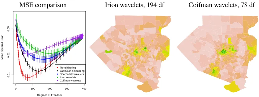
In addition to considering the wavelet design of Sharpnack et al. (2013a) for the Allegheny County example, we also considered designs of Coiman and Maggioni (2006)—a classic method that builds diffusion wavelets on a graph, and Irion (2015)—a more recent graph wavelet construction. In con-trast to Sharpnack et al. (2013a), which produces a single signal-independent orthogonal basis for a graph, both Coiman and Maggioni (2006); Irion (2015) build wavelet packets from a given graph structure. A wavelet packet is an overcomplete basis indexed by a hierarchical data structure that can be used to generate an exponential number of orthogonal bases. This construction is computa-tionally expensive as it typically involves computing eigendecompositions of large matrices. Once the wavelet packet has been constructed, for each input signal that one observes over the graph in question, one runs a “best basis” algorithm to choose a particular orthogonal basis from the wavelet packet by optimizing a particular cost function of the eventual wavelet coefficients. This is based on a message-passing-like dynamic programming algorithm, and can be quite efficient. Lastly, the denoising procedure is defined as usual (e.g., as in Donoho and Johnstone (1995)), namely, one performs the basis transformation, soft-thresholds (or hard-thresholds) the coefficients, and then reconstructs the denoised signal.

In our experiments, we used the wavelet implementations released by the authors of Coiman and Maggioni (2006); Irion (2015) with their default settings. In particular, the former implementation of Coiman and Maggioni (2006) builds wavelets from a diffusion operator constructed from the adjacency matrix of a graph, and the cost function for the best basis is defined by the`1 norm of

the wavelet coefficients. The latter implementation of Irion (2015) uses a more exhaustive search, building wavelet packets through a hierarchical partitioning and eigentransform of three different Laplacian matrices and a fourth generalized Haar-Walsh transform (GHWT), then choosing the best basis from all four collections by optimizing a meta cost function of the`p norm of wavelet coefficients overp ∈ {0.1,0.2, . . .2}. This is the “cumulative relative error” defined in equation (7.5) of Irion (2015).

(26)

MSE comparison Irion wavelets, 194 df Coifman wavelets, 78 df

0 100 200 300 400

0.01

0.02

0.05

Degrees of Freedom

Mean Squared Error

● ● ● ● ● ● ● ● ● ● ● ● ● ● ● ● ● ● ● ● ● ● ● ● ● ● ● ● ● ● ● ● ● ● ● ● ● ● ● ● ● ● ● ● ● ● ● ● ● ● ● ● ● ● ● ● ● ● ● ● ● ● ● ● ● ● ● ● ● ● ● ● ● ● ● ● ● ● ● ● ● ● ● ● ● ● ● ● ● ● ● ● ● ● ● ● ● ● ● ● ● ● ● ● ● ● ● ● ● ● ● ● ● ● ● ● ● ● ● ● ● ● ● ● ● ● ● ● ● ● ● ● ● ● ● ● ● ● ● ● ● ● ● ● ● ● ● ● ● ● ● ● ● ● ● ● ● ● ● ● ● ● ● ● ● ● ● ● ● ● ● ● ● ● ● ● ● ● ● ● ● ● ● ● ● ● ● ● ● ● ● ● ● ● ● ● ● ● ● ● ● ● ● ● ● ● ● ● ● ● ● ● ● ● ● ● ● ● ● ● ● ● ● ● ● ● ● ● ● ● ● ● ● ● ● ● ● ● ● ● ● ● ● ● ● ● ● ● ● ● ● ● ● ● ● ● ● ● ● ● ● ● ● ● ● ● ● ● ● ● ● ● ● ● ● ● ● ● ● ● ● ● ● ● ● ● ● ● ● ● ● ● ● ● ● ● ● ● ● ● ● ● ● ● ● ● ● ● ● ● ● ● ● ● ● ● ● ● ● ● ● ● ● ● ● ● ● ● ● ● ● ● ● ● ● ● ● ● ● ● ● ● ● ● ● ● ● ● ● ● ● ● ● ● ● ● ● ● ● ● ● ● ● ● ● ● ● ● ● ● ● ● ● ● ● ● ● ● ● ● ● ● ● ● ● ● ● Trend filtering Laplacian smoothing Sharpnack wavelets Irion wavelets Coifman wavelets

Figure 8: Additional wavelet analysis of the Allegheny County example.

A.2 Facebook Graph Example

Again, we consider the designs of Coiman and Maggioni (2006); Irion (2015) for the Facebook graph example of Section 5.1. Due to practical reasons, we had to change some of the default settings in the implementations provided by the authors of these wavelet methods; in the wavelet implementation of Coiman and Maggioni (2006), we took the power of the diffusion operator to be 1 instead of 4 (since the latter choice threw an error in the provided code); and in the wavelet implementation of Irion (2015), we used another “best basis” algorithm that only searches within the basis collection from the GHWT eigendecomposition, as the original algorithm was too slow due to the larger scale considered in this example. (In most examples in Irion (2015), the chosen bases come from the GHWT eigendecomposition.) We view these changes as minor, because when the same changes were applied to the methods of Coiman and Maggioni (2006); Irion (2015) on the smaller Allegheny County example, there are no obvious differences in the results.

Figure 9 shows the results for the two new wavelet methods on the Facebook graph simulation, using the same setup as in Figure 5. Once again, we find that the spanning tree wavelets of Sharp-nack et al. (2013a) perform better or on par with the other two wavelet methods across essentially all scenarios.

Appendix B. Proofs of Theoretical Results

Here we present proofs of our theoretical results presented in Sections 3 and 6.

B.1 Proof of Lemma 1

For evenk, we have∆(k+1)=DLk/2, so ifAdenotes a subset of edges, then∆(₋k_A+1)=D−ALk/2. Recall that for a connected graph, null(L) = span{1}, and the same is true for any power ofL. This means that we can write

(27)

Dense Poisson equation Sparse Poisson equation

-30 -25 -20 -15 -10 -5 0 5 10

-40 -35 -30 -25 -20 -15 -10 -5 0

Trend filtering k=0 Trend filtering k=1 Trend filtering k=2 Laplacian smoothing Sharpnack wavelets Coifman wavelets Irion wavelets

-30 -25 -20 -15 -10 -5 0 5 10

-40 -35 -30 -25 -20 -15 -10 -5 0

Inhomogeneous random walk

-30 -25 -20 -15 -10 -5 0 5 10

-40 -35 -30 -25 -20 -15 -10 -5 0

Figure 9: Additional wavelet analysis of the Facebook graph example.

Note that if1>u= 0, thenv=Lk2u ⇐⇒ u= (L†) k