Consistent Model Selection Criteria on High Dimensions

(1)

Consistent Model Selection Criteria on High Dimensions

Yongdai Kim [email protected]

Department of Statistics Seoul National University Seoul 151-742, Korea

Sunghoon Kwon [email protected]

School of Statistics University of Minnesota Minneapolis, MN 55455, USA

Hosik Choi [email protected]

Department of Informational Statistics Hoseo University

Chungnam 336-795, Korea

Editor: Xiaotong Shen

Abstract

Asymptotic properties of model selection criteria for high-dimensional regression models are stud-ied where the dimension of covariates is much larger than the sample size. Several sufficient condi-tions for model selection consistency are provided. Non-Gaussian error distribucondi-tions are considered and it is shown that the maximal number of covariates for model selection consistency depends on the tail behavior of the error distribution. Also, sufficient conditions for model selection consistency are given when the variance of the noise is neither known nor estimated consistently. Results of simulation studies as well as real data analysis are given to illustrate that finite sample performances of consistent model selection criteria can be quite different.

Keywords: model selection consistency, general information criteria, high dimension, regression

1. Introduction

Model selection is a fundamental task for high-dimensional statistical modeling where the number of covariates can be much larger than the sample size. In such cases, classical model selection criteria such as the Akaike information criterion or AIC (Akaike, 1973), the Bayesian information criterion or BIC (Schwarz, 1978) and cross validations or generalized cross validation (Craven and Wahba, 1979; Stone, 1974) tend to select more variables than necessary. See, for example, Broman and Speed (2002) and Casella et al. (2009). Also, Yang and Barron (1998) discussed severe selection bias of AIC which damages predictive performance for high-dimensional models.

(2)

sample size. Some sparse penalized approaches including the LASSO (Least Absolute Shrinkage and Selection Operator) (Tibshirani, 1996) and SCAD (Smoothly Clipped Absolute Deviation) (Fan and Li, 2001) are proven to be consistent for high-dimensional models. See Zhao and Yu (2006) for the LASSO and Kim et al. (2008) for the SCAD.

In this paper, we study asymptotic properties of a large class of model selection criteria based on the generalized information criterion (GIC) considered by Shao (1997). The class of GICs is large enough to include many well known model selection criteria such as the AIC, BIC, modified BIC by Wang et al. (2009), risk inflation criterion (RIC) by Foster and George (1994), modified risk inflation criterion (MRIC) by Foster and George (1994), corrected RIC by Zhang and Shen (2010). Also, as we will show, the extended BIC by Chen and Chen (2008) is asymptotically equivalent to a GIC.

We give sufficient conditions for a given GIC to be consistent. Our sufficient conditions are general enough to include cases where the error distribution can be other than Gaussian and the variance of the error distribution is not consistently estimated. For a case of the Gaussian error distribution with consistent estimator of the variance, our sufficient conditions include most of the previously proposed consistent model selection criteria such as the modified BIC (Wang et al., 2009), extended BIC (Chen and Chen, 2008) and corrected RIC (Zhang and Shen, 2010).

For high-dimensional models, it is not practically feasible to find the best model among all pos-sible submodels since the number of submodels are too large. A simple remedy is to find a sequence of submodels with increasing complexities (e.g., increasing number of covariates) and find the best model among them using a given model selection criterion. Examples of constructing a sequence of submodels are the forward selection procedure and solution paths of penalized regression ap-proaches. Our sufficient conditions are still valid as long as the sequence of submodels includes the true model with probability converging to 1. We discuss more on these issues in Section 4.1.

The paper is organized as follows. In Section 2, the GIC is introduced. In Section 3, sufficient conditions for the consistency of GICs are given. Various remarks about application of GICs to real data analysis are given in Section 4. In Section 5, results of simulations as well as a real data analysis are presented, and concluding remarks follow in Section 6.

2. Generalized Information Criterion

Let

L

₌_{₍_y₁_,x₁₎_{, . . . ,}₍_yn,xn₎_}_{be a given data set of independent pairs of response and covariates,} where yi∈R and xi∈Rpn.Suppose the true regression model for(y,x)is given as

y=x′β∗+ε,

whereβ∗_∈Rpn_,_E₍ε_{) =}_{0 and Var}₍ε_{) =}σ2_._{For simplicity, we assume that}σ2_{is known. For unknown}

σ2_,_{see Section 4.2.} Let Yn= (y1, . . . ,yn)

′

and Xn be the n×pn dimensional design matrix whose jth column is Xnj= (x1 j, . . . ,xn j)

′

.For givenβ_∈Rpn_,_let

Rn(β) =_kYn₋Xnβ_k2,

where_{k · k}is the Euclidean norm. For a given subsetπ_{⊂ {}1, . . . ,pn_},let ˆ

(3)

For a given sequence of positive numbers{λn},the GIC indexed by{λn}, denoted by GICλn, gives a sequence of random subsets ˆπ_λ_n of_{1, . . . ,pn_}defined as

ˆ

π_λ_n =argmin_π_⊂{₁_,...,p_n_}Rn(βˆ_π) +λn|π|σ2,

where_|π_|is the cardinality ofπ.The AIC corresponds toλn=2,the BIC toλn=log n,the RIC of

Foster and George (1994) toλn=2 log pn,the RIC of Zhang and Shen (2010) toλn=2(log pn+

log log pn).Shao (1997) studied the asymptotic properties of the GIC focusing on the AIC and BIC.

When pnis large, it would not be wise to search all possible subsets of{1, . . . ,pn}.Instead, we

set an upper bound on the cardinality ofπ,say snand search the optimal model among submodels

whose cardinalities are smaller than sn. Chen and Chen (2008) considered a similar model selection

procedure. Let

M

sn ₌_{π_{⊂ {}₁_{, . . . ,}_pn_}_:_|π_{| ≤}_sn_}_._{We define the restricted GIC}

λn as ˆ

π_λn=argminπ∈MsnRn(βˆπ) +λn|π|σ

2_. ₍₁₎

The restricted GIC is the same as the GIC if sn=pn.In the following, we will only consider the

restricted GIC and suppress the term “restricted” unless there is any confusion.

3. Consistency of GIC on High Dimensions

Letπ∗_n=_{j :_|β∗_j_{| 6}=0_}.We say that the GIC_λ_n is consistent if Pr(πˆ_λ_n =π∗_n)_→1

as n_→∞.In this section, we prove the consistency of the GIC_λ_n under regularity conditions. For a given subsetπof_{1, . . . ,pn},let Xπ= (Xnj,j∈π)be the n× |π|matrix whose columns

consist of Xnj,j∈π.For a given symmetric matrix A,letξ(A)be the smallest eigenvalue of A. 3.1 Regularity Conditions

We assume the following regularity conditions.

• A1 : There exists a positive constant M1such that Xnj′Xnj/n≤M1for all j=1, . . . ,pnand all

n.

• A2 : There is a positive constant M2such thatξ(X

′ π∗

nXπ∗n/n)≥M2for all n.

• A3 : There exist positive constants c1and M3such that 0≤c1<1/2 andρn≥M3n−c1,where

ρn= inf

π:|π|≤sn

ξ(X′_πX_π/n).

• A4 : There exist positive constants c2and M4such that 2c1<c2≤1 and

n(1−c2)/2_min

j∈π∗

n

|β∗j| ≥M4.

(4)

Condition A1 assumes that the covariates are bounded. Condition A2 means that the design matrix of the true model is well posed. Condition A3 is called the sparse Riesz condition and used in Chen and Chen (2008), Zhang (2010) and Kim and Kwon (2012). Condition A4 and A5 allow the nonzero regression coefficients to converge to 0 and the number of signal variables to diverge, respectively.

Remark 1 Condition A3 implies that sn≤n.

3.2 The Main Theorem

The following theorem proves consistency of the GIC_λ_n.The proofs are deferred to Appendix.

Theorem 2 Suppose E(ε2k₎_<∞_{for some integer k}_>₀_._Ifλ

n=o(nc2−c1) and pn/(λnρn)k→0, then the GIC_λ_n is consistent.

In Theorem 2, pn can diverge only polynomially fast in n since pn=o(λnk) =o(nkc2).Since k

can be considered as a degree of tail lightness of the error distribution, we can conclude that the lighter the tail of the error distribution is, the more covariates the GIC_λ_n is consistent with. When

ε is Gaussian, the following theorem proves that the GIC_λ_n can be consistent when pn diverges

exponentially fast.

Theorem 3 Suppose ε _∼ N(0,σ2₎_. _If _λ

n = o(nc2−c1),snlog pn = o(nc2−c1) and

λn−2 log pn−log log pn→∞,then the GICλn is consistent.

In the following, we give three examples for (i) fixed pn,(ii) polynomially diverging pn and

(iii) exponentially diverging pn. For simplicity, we let c1 =0 (i.e., ρn≥M3 >0), c2=1 (i.e., minj∈π∗

n|β∗j|>0) and c3=0 (i.e., qnis fixed). In addition, we let snbe fixed.

Example 1 Consider a standard case where pnis fixed and n goes to infinity. Theorem 2 implies that the GIC_λ_n is consistent if λn/n→0 and λn→∞ regardless of the tail lightness (i.e., k) of the error distribution, provided the variance exists. The BIC, which is the GIC with λn=log n, satisfies these conditions and hence is consistent. Note that the AIC does not satisfy the conditions in Theorem 2. Any GIC with λn =nc,0<c<1 is consistent, which suggests that the class of consistent model selection criteria is quite large. See Shao (1997) for more discussions.

Example 2 Consider a case of pn=nγ,γ>0. The GIC with λn=nξ,0<ξ<1 andγ<kξ is consistent. That is, for larger pn,we need largerλn for consistency, which is reasonable because we need to be more careful not to overfit when pnis large. When the error distribution is Gaussian, Theorem 3 can be compared with other previous results of consistency. First, the BIC (i.e., the GIC with λn=log n) is consistent when γ<1/2.For 0<γ<1,Theorem 3 implies that the modified BIC of Wang et al. (2009), which is a GIC withλn=log log pnlog n,is consistent. Chen and Chen (2008) proposed a model selection criterion called the extended BIC given by

ˆ

πeBIC₌_argmin

π⊂{1,...,pn},|π|≤KRn( ˆ

βπ) +_|π_|σ2log n+2κσ2log

pn

|π|

for some K>0 and 0_≤κ_≤1,and proved that the extended BIC is consistent whenκ>1₋1/(2γ). Since log pn

|π|

≍ |π|log pnfor|π| ≤K,we have

|π|σ2log n+2γσ2log

pn

|π|

(5)

Hence, Theorem 3 confirms the result of Chen and Chen (2008).

Example 3 When the error distribution is Gaussian, the GIC can be consistent for exponentially increasing pn (i.e., ultra-high dimensional cases). The GIC withλn=nξ,0<ξ<1 is consistent when pn=O(exp(αnγ)) for 0<γ<ξ andα>0.Also, it can be shown by Theorem 3 that the extended BIC withγ=1 is consistent with pn=O(exp(αnγ))for 0<γ<1/2.The consistency of the corrected RIC of Zhang and Shen (2010) can be confirmed by Theorem 3, but the regularity conditions for Theorem 3 are more general than those of Zhang and Shen (2010).

4. Remarks

Remarks regarding to applications of the GIC to real data analysis are given.

4.1 Construction of Sub-Models

For high-dimensional models, it is computationally infeasible to search the optimal model among all possible submodels. A simple remedy is to construct a sequence of submodels and select the optimal model among the sequence of submodels. Examples of constructing a sequence of submodels are the forward selection (Wang, 2009) and the solution path of a sparse penalized estimator obtained by, for example, the Lars algorithm (Efron et al., 2004) or the PLUS algorithm (Zhang, 2010). The following algorithm exemplifies the model selection procedure with the GIC and a sparse penalized regression approach.

• For a given sparse penalty Jη(t) indexed by η_≥0, find the solution path of a penalized estimator_{βˆ(η):η>0_},where

ˆ

β(η) =argmin_β Rn(β) +

p

∑

j=1

J_η(_|βj|) !

.

The LASSO corresponds to Jη(t) =ηt and the SCAD penalty corresponds to J_η(t) = ηtI(0_≤0<η)

+

aη(t₋η)₋(t2₋η2)/2

a₋1 +η

2

I(η_≤t<aη)

+

(a₋1)η2 2 +η

2

I(t_≥aη)

for some a>2.

• Let S(η) =_{j : ˆβ(η)j6=0}andϒ={η: S(η)6=S(η−),|S(η)| ≤sn}.

• Apply the GIC_λ_n to S(η),η_∈ϒto select the optimal model. That is, let ˆπ_λ_n=S(η∗₎_where

η∗₌_argmin

η∈ϒ

Rn(βˆη) +λn|S(η)|

and

ˆ

(6)

It is easy to see that a consistent GIC is still consistent with a sequence of sub-models as long as the sequence of submodels includes the true model with probability converging to 1. For the LASSO solution path, Zhao and Yu (2006) proved the selection consistency under the irrepresentable con-dition, which is almost necessary (Zou, 2006). However, the irrepresentable condition is hardly satisfied for high-dimensional models. The consistency of the solution path of a nonconvex penal-ized estimator with either the SCAD penalty or minimax concave penalty is proved by Zhang (2010) and Kim and Kwon (2012). By combining Theorem 4 of Kim and Kwon (2012) and Theorem 2 of the current paper, we can prove the consistency of the GIC with the solution path of the SCAD penalty or minimax concave penalty, which is formally stated in the following theorem.

Theorem 4 Condition A3 is replaced by A3’, where

• A3’: There exist positive constants c1and M3such that 0≤c1<1/2 andρn≥M3nc1/2.

Suppose E(ε2k₎_<_∞_{for some integer k}_>₀_._{If p}

n=o(nk(c2/2−c1)),the under the regularity conditions A1 to A5 with A3 being replaced by A3’, the solution path of the SCAD or minimax concave penalty included the true model with probability converging to 1, and hence the GIC_λ_n withλn=o(nc2−c1) is consistent with the solution path of the SCAD or minimax concave penalty.

Remark 5 Condition A3’ is a technical modification needed for Theorem 4 of Kim and Kwon (2012). Note that A3 is weaker than A3’, which is an advantage of using the l0 penalty rather

than nonconvex penalties which are linear around 0.

Remark 6 Theorem 3 can be modified similarly for the GIC with the solution path of the SCAD or minimax concave penalty, since Theorem 4 of Kim and Kwon (2012) can be modified accordingly for the Gaussian error distribution.

4.2 Estimation of the Variance

To use the GIC in practice, we need to knowσ2.Ifσ2is unknown, we can replace it by its estimate. Theorems 2 and 3 are still valid as long asσ2 is estimated consistently. When pnis fixed, we can

estimateσ2consistently by the mean squared error of the full model. For high-dimensional data, it is not obvious how to estimateσ2.However, a weaker condition can be put on an estimator ˆσ2of

σ2_{for the GIC to be consistent. Suppose that}

0<rin f =lim inf

ˆ

σ2

σ2 ≤lim sup ˆ

σ2

σ2 =rsup<∞ (2)

with probability 1. This condition essentially assumes that ˆσ2is neither too small nor too large. It is not difficult to show that Theorem 2 is still valid with ˆσ2 satisfying (2). This, however, is not true for Theorem 3. A slightly weak version of Theorem 3 which only requires (2) is given in the following theorem.

Theorem 7 Suppose ε_∼N(0,σ2₎_._{Let ˆ}σ2 _{be an estimator of} σ2 _{satisfying (2). If} λ

n=o(nc2−c1) andλn−2M1log pn/ρnrin f →∞,then the GICλn with the estimated variance is consistent.

The corrected RIC, the GIC withλn=2(log pn+log log pn), does not satisfy the condition in

(7)

4.3 The Size of sn

For condition A5, sn should be large enough so that qn≤sn.In many cases, sncan be sufficiently

large for practical purposes. For example, suppose_{xi,i≤n}are independent and identically

dis-tributed pndimensional random vectors such that E(x1) =0 and Var(x1) =Σ= [σjk].For a given

ρ>0,let s∗be the largest integer such that the smallest eigenvalue ofΣη= [σjk,j,k_∈η]is greater than ρfor any η_{⊂ {}1, . . . ,pn} with|η| ≤s∗.For example, whenΣis compound symmetry, that

is σj j =1 and σjk =ν for j6=k and ν∈[0,1), the smallest eigenvalue of Ση is 1−ν for all

η_{⊂ {}1, . . . ,pn_}and hence s∗=pn if 1₋ν>ρ.Let A=Ση−X′_ηXη/n.By the inequality (2) in Greenshtein and Ritov (2004), we have

sup

j,k

n

∑

i=1

xi jxik/n−σjk

=Op r

log n

n !

,

and hence sup_jk|ajk|=Op( p

log n/n),where ajk is the(j,k)entry of A.Since the largest

eigen-value of A is bounded by _|η_|Op(plog n/n), the smallest eigenvalue of Xη′Xη/n is greater than

ρ− |η|Op(

p

log n/n)if_|η_{| ≤}s∗.So, we can let sn=min{nc,s∗}for c<1/2. 5. Numerical Analysis

In this section, we investigate finite sample performance of various GICs by simulation experiments as well as real data analysis. We consider the five GICs whose correspondingλns are given as

• GIC1(=BIC) :λ( 1)

n =log n,

• GIC2:λ(n2)=p1n/3,

• GIC3:λ(n3)=2 log pn,

• GIC4:λ(n4)=2(log pn+log log pn),

• GIC5:λ(n5)=log log n log pn,

• GIC6:λ(n6)=log n log pn.

The GIC1 is the BIC. By Theorem 2, the GIC2 can be consistent when E(ε8)<∞. That is, the GIC2 can be consistent when the tail of the error distribution is heavier than that of the Gaussian distribution. The GIC3and GIC4are the RIC of Foster and George (1994) and the corrected RIC of Zhang and Shen (2010). The GIC5and GIC6are consistent when the error distribution is Gaussian.

5.1 Simulation 1

The first simulation model is

y=x′β∗+ε

where x= (x1, . . . ,xp)

′

is a multivariate Gaussian random vector with mean 0 and covariances of xk

and xlbeing 0.5|k−l|. Theεis a random variable with mean 0 andσ2=4.Forβ∗= (3,1.5,0,0,2,0

′

p−5)

′

(8)

Li (2001). We consider two distributions forε: the Gaussian distribution and the t-distribution with 3 degrees of freedom multiplied by a positive constant to make the variance be 4.

First, we compare performances of the GICs applied to all possible submodels with those ap-plied to submodels constructed by the solution path of a sparse penalized approach. For a sparse penalized approach, we use the SCAD penalty with the PLUS algorithm (Zhang, 2010). Table 1 summarizes the results when p=10 and n=100 based on 300 repetitions of the simulation. In the table, ‘Signal’, ‘Noise’, ‘PTM’ and ‘Error (s.e.)’ represent the average number of variables included in the selected model among the signal variables, the average number of variables included in the selected model among noisy variables, the proportion of the true model being exactly identified, and the average of the squared Euclidean distance of ˆβπˆ_λ_n formβ∗ with the standard error in the parenthesis, respectively. From Table 1, we can see that the results based on the SCAD solution path are almost identical to those based on the all possible search, which suggests that the model selection with the SCAD solution path is a promising alternative to all possible search.

Submodels Criterion Signal Noise PTM Error (s.e.) All GIC1 3 0.22 0.80 0.220(0.013) GIC2 3 0.92 0.39 0.371(0.018) GIC3 3 0.22 0.80 0.220(0.013) GIC4 3 0.09 0.91 0.190(0.016) GIC5 3 0.39 0.67 0.267(0.016) GIC6 3 0.02 0.98 0.158(0.015) SCAD GIC1 3 0.21 0.80 0.218(0.013) GIC2 3 0.93 0.40 0.367(0.018) GIC3 3 0.21 0.80 0.218(0.013) GIC4 3 0.10 0.90 0.191(0.016) GIC5 3 0.39 0.67 0.266(0.016) GIC6 3 0.03 0.97 0.163(0.015)

Table 1: Comparison of the 6 GICs with the all possible search and SCAD solution path when

p=10 and n=100.

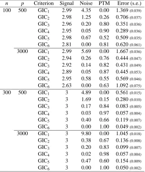
For simulation with high-dimensional models, we consider p=500 and p=3000.The results of prediction accuracy and variable selectivity for n=100 and n=300 with the error distribution being the Gaussian and t-distributions are presented in Tables 2 and 3, respectively. We use the SCAD solution path to construct a sequence of submodels. The values are the averages based on 300 repetitions of the simulation.

First of all, the GIC1 (the BIC) is the worst in terms of prediction accuracy for p=500 and

(9)

n p Criterion Signal Noise PTM Error (s.e.) 100 500 GIC1 2.99 4.35 0.00 1.369(0.039) GIC2 2.98 1.25 0.26 0.706(0.037) GIC3 2.96 0.20 0.80 0.351(0.036) GIC4 2.95 0.05 0.90 0.289(0.036) GIC5 2.98 0.67 0.52 0.509(0.035) GIC6 2.81 0.00 0.81 0.620(0.061) 3000 GIC1 2.99 5.69 0.00 1.667(0.036) GIC2 2.94 0.26 0.76 0.444(0.047) GIC3 2.92 0.14 0.82 0.431(0.049) GIC4 2.89 0.05 0.87 0.445(0.053) GIC5 2.95 0.58 0.55 0.569(0.046) GIC6 2.63 0.00 0.63 1.092(0.075) 300 500 GIC1 3 4.89 0.00 0.561(0.015) GIC2 3 1.69 0.15 0.280(0.010) GIC3 3 0.17 0.84 0.083(0.005) GIC4 3 0.03 0.97 0.057(0.004) GIC5 3 0.40 0.66 0.119(0.007) GIC6 3 0.00 1.00 0.049(0.002) 3000 GIC1 3 9.80 0.00 1.045(0.018) GIC2 3 0.38 0.67 0.136(0.008) GIC3 3 0.20 0.83 0.099(0.007) GIC4 3 0.02 0.98 0.057(0.004) GIC5 3 0.47 0.60 0.154(0.009) GIC6 3 0.00 1.00 0.050(0.002)

Table 2: Comparison of the 6 GICs with Simulation 1 when the error follows the Gaussian distri-bution.

selection criteria specialized for high-dimensional models are necessary for optimal prediction and variable selection, (ii) finite sample performances of consistent GICs are quite different, and (iii) the tail lightness of the error distribution does not affect seriously to relative performances of model selection criteria.

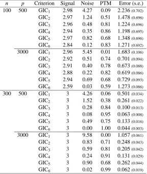
5.2 Simulation 2

We consider a more challenging case by modifying the model for Simulation 1. We divide the p components ofβ∗into continuous blocks of size 20. We randomly select 5 blocks and assign the value(3,1.5,0,0,2,0′₁₅)/1.5 to each block. The entries in other blocks are set to be zero.

(10)

Table 3: Comparison of the 6 GICs with Simulation 1 when the error follows the t-distribution.

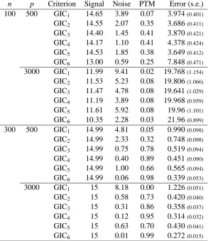
5.3 Real Data Analysis

We analyze the data set used in Scheetz et al. (2006), which consists of gene expression levels of 18,975 genes obtained from 120 rats. The main objective of the analysis is to find genes that are correlated with gene TRIM32 known to cause Bardet-Biedl syndromes. As was done by Huang et al. (2008), we first select 3000 genes with the largest variance in expression level, and then choose the top p genes that have the largest absolute correlation with gene TRIM32 among the selected 3000 genes.

We compare prediction accuracies of the 6 GICs with the submodels obtained from the SCAD solution path. Each data set was divided into two parts, training and test data sets, by randomly selecting 2/3 observations and 1/3 observations, respectively. We use the training data set to select the model and estimate the regression coefficients, and use the test data set to evaluate the prediction performance.

(11)

Table 4: Comparison of the 6 GICs with Simulation 2 when the error follows the Gaussian distri-bution.

nonzero coefficients is equal to pmax, and to estimate the error variance by the mean squared error

of the selected model. Following the results of Scheetz et al. (2006), Chiang et al. (2006), Huang et al. (2008), and Kim et al. (2008), we guess that a reasonable model size would be in between 20 and 40. Table 6 compares the 6 GICs with the number of pre-screened genes being p=500 and

p=3000, when the error variance is estimated with pmax being 20, 30 and 40, respectively. All

values are the arithmetic means of the results from 100 replicated random partitions. In the table, ‘Nonzero’ denotes the number of nonzero coefficients in the selected model and ‘Error (s.e.)’ is the prediction error on the test data set and the standard error in the parenthesis obtained on the test data. For p=500,the lowest prediction error is achieved by the GIC2and the GIC3, GIC4and GIC5 perform reasonably well with pmax=20.For p=3000,the lowest prediction error is achieved by

the GIC5with pmax=20.So, we choose pmax=20 for estimation of the error variance.

As argued by Yang (2005), the standard error obtained by random partition could be misleading. As a supplement, we draw the box plots of the 100 prediction errors of the 6 GICs with pmax=20

(12)

n p Criterion Signal Noise PTM Error (s.e.) 100 500 GIC1 14.65 3.89 0.07 3.974(0.401) GIC2 14.55 2.07 0.35 3.686(0.411) GIC3 14.40 1.45 0.41 3.870(0.421) GIC4 14.17 1.10 0.41 4.378(0.424) GIC5 14.53 1.85 0.38 3.649(0.412) GIC6 13.00 0.59 0.25 7.848(0.471) 3000 GIC1 11.99 9.41 0.02 19.768(1.154) GIC2 11.53 5.23 0.08 19.806(1.066) GIC3 11.47 4.78 0.08 19.641(1.029) GIC4 11.19 3.89 0.08 19.968(0.959) GIC5 11.61 5.92 0.08 19.96(1.101) GIC6 10.35 2.28 0.03 21.96(0.899) 300 500 GIC1 14.99 4.81 0.05 0.990(0.098) GIC2 14.99 2.33 0.32 0.748(0.098) GIC3 14.99 0.75 0.78 0.519(0.094) GIC4 14.99 0.40 0.89 0.451(0.090) GIC5 14.99 1.00 0.66 0.565(0.094) GIC6 14.99 0.06 0.98 0.339(0.053) 3000 GIC1 15 8.18 0.00 1.226(0.051) GIC2 15 0.58 0.73 0.420(0.040) GIC3 15 0.31 0.86 0.358(0.037) GIC4 15 0.12 0.95 0.314(0.032) GIC5 15 0.63 0.70 0.430(0.041) GIC6 15 0.01 0.99 0.272(0.015)

Table 5: Comparison of the 6 GICs with Simulation 2 when the error follows the t-distribution.

GIC3 and GIC5 have lower prediction errors than the GIC4 and GIC6 while the formers tend to select more variables than necessary in the simulation studies. This observation suggests that there might be many signal genes whose impacts on the response variable are relatively small.

6. Concluding Remarks

The range of consistent model selection criteria is rather large, and it is not clear which one is better with finite samples. It would be interesting to rewrite the class of GICs as_{λn=αnlog pn:αn>

0_}.The GIC3, GIC5 and GIC6 correspond toαn=2,αn=log log n and αn=log n,respectively.

When the rue model is expected to be very sparse, it would be better to letαn be rather large (e.g.,

αn=log n), while a smallerαn(e.g.,αn=2 orαn=log log n) would be better when many signal

covariates with small regression coefficients are expected to exist. The relation of the GICs with largerαnwith those with smallerαnwould be similar to the relation between the AIC and BIC for

(13)

pmax=20

p

500 3000

Error (s.e.) Nonzero Error (s.e.) Nonzero GIC1 0.742(0.038) 15.91 0.766(0.036) 18.62 GIC2 0.649(0.028) 10.95 0.686(0.035) 3.91 GIC3 0.656(0.031) 6.99 0.697(0.035) 3.69 GIC4 0.677(0.034) 5.57 0.719(0.037) 2.78 GIC5 0.664(0.030) 9.76 0.667(0.032) 4.92 GIC6 0.732(0.038) 3.03 0.792(0.039) 1.82

pmax=30

p

500 3000

Error (s.e.) Nonzero Error (s.e.) Nonzero GIC1 0.890(0.035) 27.26 0.868(0.039) 26.07 GIC2 0.825(0.038) 21.77 0.698(0.031) 14.04 GIC3 0.752(0.029) 17.53 0.696(0.031) 13.25 GIC4 0.722(0.029) 15.19 0.691(0.034) 10.76 GIC5 0.800(0.030) 20.29 0.729(0.032) 15.99 GIC6 0.688(0.030) 11.31 0.683(0.034) 5.53

pmax=40

p

500 3000

Error (s.e.) Nonzero Error (s.e.) Nonzero GIC1 1.040(0.077) 34.54 0.936(0.041) 33.80 GIC2 0.916(0.036) 29.59 0.892(0.041) 27.27 GIC3 0.859(0.035) 25.10 0.878(0.040) 26.37 GIC4 0.846(0.039) 23.02 0.846(0.038) 25.00 GIC5 0.890(0.035) 28.20 0.910(0.040) 28.60 GIC6 0.763(0.029) 18.69 0.800(0.037) 21.02

Table 6: Comparison of the 6 GICs with the gene expression data. The bold face numbers represent the lowest prediction errors among the 6GICs.

Estimation of σ2 is an open question. We may use the BIC-like criterion by assuming the Gaussian distribution:

ˆ

π_λn=argminπ⊂{1,...,pn}log(Rn(βˆπ)/n) +λn|π|.

If Rn(βˆπ)/n is bounded above from ∞ and below from 0 in probability (uniformly in π and n),

(14)

0.5 1.0 1.5 2.0

GIC1 GIC2 GIC3 GIC4 GIC5 GIC6

(a) p=500

0.5 1.0 1.5 2.0

GIC1 GIC2 GIC3 GIC4 GIC5 GIC6

(b) p=3000

Figure 1: The boxplot of the prediction errors when (a) p=500 and (b) p=3000 with pmax=20.

For consistency, the smallest eigenvalue of the design matrix of the true model is assumed to be sufficiently large (i.e., condition A2). However, it is frequently observed for large dimensional data that some covariates are highly correlated and they affect the output similarly. In this case, selecting some covariates and ignoring the others, which is done by a standard model selection method, is not optimal. See Zou and Hastie (2005) for an example. It would be interesting to develop consistent model selection methods for such cases.

Acknowledgments

This research was supported by the National Research Foundation of Korea grant number 20100012671 funded by the Korea government.

Appendix A. Proof of Theorem 2

Without loss of generality, we letπ∗_n=_{1, . . . ,qn_}.Let ˆβ∗=βˆπ∗

n.Let ˆYπ=Xnβˆπand ˆYn∗=Xnβˆπ∗n. We let β∗= (β(1)∗_,_β(2)∗₎_,_where _β(1)∗ _∈_Rqn _and β(2)∗ _∈_Rpn−qn_._{Let C}

n=X

′

nXn/n and C(ni,j)= Xn(i)′Xn(j)/n for i,j=1,2.We need the following two lemmas.

Lemma 8

max

j≤qn| ˆ

β∗

j−β∗j|=op(n−(1−c2)/2).

Proof. Let zj=√n(βˆ∗j−β∗j).For proving Lemma 8, we will show

max

j≤qn|

(15)

Write

z= (C(n1,1))−1 X(n1)′εn

√

n =H

(1)′ εn,

where z= (z1, . . . ,zqn)

′

,εn= (ε1, . . . ,εn)

′

and H(1)′ = (h₁(1), . . . ,h(q1n))

′

= (C(n1,1))−1X(1)

′

n /√n.Since H(1)′H(1)= (C(n1,1))−1,A2 of the regularity conditions implieskh(j1)k22≤1/M2for all j≤qn.Hence, E(zj)2k<∞for all j≤qnsince E(εi)2k<∞.Thus

Pr(_|zj|>t) =O(t−2k).

For anyη>0,we can write

Pr(_|zj|>ηnc2/2for some j=1, . . . ,qn) ≤ qn

∑

j=1

Pr(_|zj|>ηnc2/2)

≤

qn

∑

j=1 1

ηn−c2k

= 1

ηqnn−c2k≤

1

ηn−(c2−c3)k→0,

which completes the proof.

Lemma 9

max

qn<j≤pn|

<Yn₋Yˆ_n∗,X_nj>_|=op(pnλnρn).

Proof. Note that

(<Yn₋Yˆ_n∗,X_nj>,j=qn+1, . . . ,pn) = X(n2)′

Yn₋X(n1)βˆ∗(1)

= X(n2)′

Yn−X(n1)

1

n(C

(1,1)

n )−1X(1)

′

n Yn

= X(n2)′

X(n1)β∗(1)+εn−X(n1)

1

n(C

(1,1)

n )−1X(1)

′

n (X(n1)β∗(1)+εn)

= X(n2)′

I₋1 nX

(1)

n (C(n1,1))−1X(1)

′

n

εn.

Hence, we have

<Yn−Yˆn∗,Xnj> /

√

n=h(_j2)′εn for j=qn+1, . . . ,pn, (3)

where h(_j2)is the j₋qncolumn vector of H(2)and

H(2)′ =Cn(2,1)(C(n1,1))−1

1 √

nX

(1)′

n −

1 √

nX

(2)′

n .

Note that

H(2)′H(2)=1

nX

(2)′

n

I₋X(n1)(X(1)

′

n X(n1))−1X(1)

′

n

(16)

Since the all eigenvalues of I₋X(n1)(X(1)

′

n X(n1))−1X(1)

′

n are between 0 and 1, we havekh(_j2)k2₂≤M1 for all j=qn+1, . . . ,pn.Hence, E(ξj)2k<∞,whereξj=<Yn−Yˆn∗,X

j

n > /√n,and so Pr(_|ξj|>t) =O(t−2k).

Finally, for anyη>0,

Pr

|<Yn−_Yˆ∗

n,Xnj>|>η p

nλnρnfor some j=qn+1, . . . ,pn

= Pr

|ξj|>η p

λnρnfor some j=qn+1, . . . ,pn

≤

pn

∑

j=qn+1 Pr

|ξj|>η p

λnρn

= (pn−qn)O

1 (λnρn)k

=O

pn

(λnρn)k

→0,

which completes the proof.

Proof of Theorem 2. For anyπ,we can write

Rn(βˆπ) +λn|π|σ2−Rn(βˆ∗)−λn|π∗n|σ2

=₋2∑pn

j=qn+1 ˆ

βπ,j<Yn−Yˆn∗,Xj>+(βˆπ−βˆ∗)

′

(X′_nXn)(βˆπ−βˆ∗) +λn(|π| − |π∗n|)σ2.

By Condition A3,

(βˆπ−βˆ∗)′(X_n′Xn)(βˆπ−βˆ∗)_≥

∑

j∈π∪π∗

nρn(βˆπ,j−βˆ∗j)2.

Hence, we have for anyπ_∈

M

sn_,

Rn(βˆπ) +λn|π|σ2−Rn(βˆ∗)−λn|π∗n|σ2≥

∑

j∈π∪π∗

n

wj,

where

wj=−2 ˆβπ,j<Yn−Yˆn∗,Xnj>I(j6∈π∗n) +nρn(βˆπ,j−βˆ∗j)2+λn(I(j∈π−π∗n)−I(j∈π∗n−π))σ2.

For j∈π∗

n−π,we have wj=nρnβˆ∗j2−λnσ2.Let

An={nρnβˆ∗j2−λnσ2>0,j=1, . . . ,qn}. (4)

Then, Pr(An)_→1 by Lemma 8 and Conditions A3 and A4. For j_∈π₋π∗_n

wj = −2 ˆβπ,j<Yn−Yˆn∗,Xnj>+nρnβˆ2π,j+λnσ2

≥ −<Yn−Yˆn∗,Xnj>2/(nρn) +λnσ2.

Let

(17)

Then, Pr(Bn)_→1 by Lemma 9. For j_∈π_∩π∗_n,

wj=nρn(βˆπ,j−βˆ∗j)2≥0.

To sum up, on An∩Bn,

Rn(βˆπ) +λn|π|σ2−Rn(βˆ∗)−λn|π∗n|σ2>0

for allπ₆=π∗_n.Since Pr(An_∩Bn)_→1,the proof is done.

Appendix B. Proof of Theorem 3

For givenπ_{⊂ {}1, . . . ,pn},let Mπbe the projection operator onto the space spanned by(X(j),j∈π).

That is, M_π=X_π(X′_πX_π)−1_X′

πprovided Xπis of full rank. Let Xnβ∗n=µnand I be the n×n identity

matrix. Without loss of generality, we assumeσ2=1.

Lemma 10 There existsη>0 such that for anyπ_∈

M

sn _withπ∗

n*π,

µ′_n(I₋Mπ)µ_n_≥η_|π−_|nc2−c1_,

whereπ−=π∗

n−π.

Proof. For givenπ_∈

M

sn _withπ∗

n*π,we have µ′_n(I₋Mπ)µ_n

= inf

α∈R|π|k

X_π−β∗_π−−Xπαk2

= inf

α∈R|π|(β

∗′ π−,α

′

)(X_π−,Xπ) ′

(X_π−,Xπ)(β∗ ′ π−,α

′

)′

≥ nkβ∗π−k2ρn

≥ M3M4|π−|nc2−c1,

whereβ∗_π−= (β∗j,j∈π−)and the last inequality is due to Condition A4.

Lemma 11 For givenπ_{⊂ {}1, . . . ,pn_},let

Zπ= µ ′

n(I−Mπ)εn p

µ′_n(I₋M_π)µ_n.

Then

max

π∈Msn|Zπ|=Op( p

snlog pn).

Proof. Note that Zπ∼N(0,1)for allπ_∈

M

sn_._Since

(18)

for some C>0,we have Pr

max

π∈Msn|Zπ|>t

≤

∑

π∈Msn

C exp(₋t2/2)

≤ C psn

n exp(−t2/2).

Hence, if we let t=√wsnlog pn,

Pr

max

π∈Msn|Zπ|>t

≤C exp((₋w/2+1)snlog pn)→0

as w_→∞.

Lemma 12

max

π∈Msnε

′

nMπεn=Op(snlog pn).

Proof. For givenπ_{⊂ {}1, . . . ,pn},let r(p)be the rank of Xπ.Note thatε

′

nMπεn∼χ2(r(π))where

χ2₍_k₎_{is the chi-square distribution with degree of freedom k}_._{It is easy to see that (see, for example,} Yang 1999)

Pr(ε′_nMπεn≥t)≤exp

−t−₂r(π) _r₍t_π₎ r(π)/2

. (7)

Hence

Pr

max

π∈Msnε

′

nMπεn≥t

≤

sn

∑

k=1

pn

k

Pr(Wk≤t),

where Wk∼χ2(k).Since Pr(Wk≥t)≤Pr(Wsn≥t),we have

Pr

max

π∈Msne

′

nMπen≥t

≤ Pr(Wsn ≥t)

sn

∑

k=1

pn

k

≤ Pr(Wsn ≥t)p

sn

n. (8)

The proof is done by applying (7) to (8).

Proof of Theorem 3. First, we will show that Pr(π∗

n *πˆλn)→0.For given π⊂ {1, . . . ,pn},let

Rn(π) =Rn(βˆπ).Note that Rn(π) =Y

′

n(I−Mπ)Yn.Forπ+π∗n,Lemmas 10, 11 and 12 imply Rn(π)−Rn(π∗n) +λn(|π| − |π∗n|)σ2

= µ′_n(I₋M_π)µ_n+2µ′_n(I₋M_π)εn+ε

′

n(Mπ∗−Mπ)εn+λn(|π| − |π∗n|)σ2

≥ η|π−|nc2−c1₋₂pη_|π−_|_nc2−c1_Op(p_sn_{log p}_n)−_Op(_sn_{log p}_n)− |π−|λn, whereπ−=π∗

n−π.Since snlog pn≤o(nc2−c1)andλn=o(nc2−c1),the proof is done.

It remains to show that the probability of inf

π∈Msn_,_π_!_π∗

n

(19)

converges to 1. By Theorem 1 of Zhang and Shen (2010), the probability of (9) is larger than

2₋

1+e1/2exp

−λn−₂logλn

pn−qn

,

which converges to 1 when 2 log pn−λn+logλn→ −∞.The equivalent condition with 2 log pn−

λn+logλn→ −∞isλn−2 log pn−log log pn→∞.

Appendix C. Proof of Theorem 4

By Theorem 4 of Kim and Kwon (2012), the solution path of the SCAD or minimax concave penalty include the true model with probability converging to 1. Since condition A3’ is stronger than condition A3, the GIC_λ_n withλn=o(nc2−c1)is consistent, and so is with the solution path of

the SCAD or minimax concave penalty.

Appendix D. Proof of Theorem 7

Let ˜Anand ˜Bnbe the sets defined in (4) and (5) except thatσ2is replaced by ˆσ2.It suffices to show that Pr(_A˜_n_∩_B˜_n₎_→₁_._{It is not difficult to prove Pr}₍_A˜_n₎_→_{1 by Lemma 8 and (2).}

For ˜Bn,sinceεi∼N(0,σ2),(3) implies <Yn−_Yˆ∗

n,Xnj> /

√

n∼N(0,σ2

j)

whereσ2_j_≤σ2M1.By (6), we have Pr(_B˜c

n) ≤ Pr(<Yn−Yˆn∗,Xnj>2>nρnλnσˆ2for some j=qn+1, . . . ,pn)

≤ C pnexp(₋ρnrin fλn/2M1).

Hence, as long as 2M1log pn/(ρnrin f)−λn→ −∞,Pr(B˜cn)→0 and the proof is done.

References

H. Akaike. Information theory and an extension of the maximum likelihood principle. In B. N. Petrox and F. Caski, editors, Second International Symposium on Information Theory, volume 1, pages 267–281. Budapest: Akademiai Kiado, 1973.

K. W. Broman and T. P. Speed. A model selection approach for the identification of quantitative trait loci in experimental crosses. Journal of the Royal Statistical Society, Ser. B, 64:641–656, 2002.

G. Casella, F. J. Giron, M. L. Martinez, and E. Moreno. Consistency of bayesian procedure for variable selection. The Annals of Statistics, 37:1207–1228, 2009.

(20)

A. P. Chiang, J. S. Beck, H.-J. Yen, M. K. Tayeh, T. E. Scheetz, R. Swiderski, D. Nishimura, T. A. Braun, K.-Y. Kim, J. Huang, K. Elbedour, R. Carmi, D. C. Slusarski, T. L. Casavant, E. M. Stone, and V. C. Sheffield. Homozygosity mapping with snp arrays identifies a novel gene for bardet-biedl syndrome (bbs10). Proc. Nat. Acad. Sci., 103:6287–6292, 2006.

P. Craven and G. Wahba. Smoothing noisy data with spline functions: Estimating the correct degree of smoothing by the method of generalized cross validation. Numer. Math., 31:377–403, 1979. B. Efron, T. Hastie, I. Johnstone, and R. Tibshirani. Least angle regression. The Annals of Statistics,

32:407–499, 2004.

J. Fan and R. Li. Variable selection via nonconcave penalized likelihood and its oracle properties.

Journal of the American Statistical Association, 96:1348–1360, 2001.

D. P. Foster and E. I. George. The risk inflation criterion for multiple regression. The Annals of

Statistics, 22:1947–1975, 1994.

E. Greenshtein and Y. Ritov. Persistence in high-dimensional linear predictor selection and the virtue of overparametrization. Bernoulli, 10:971–988, 2004.

J. Huang, S. Ma, and C-H. Zhang. Adaptive lasso for sparse high-dimensional regression models.

Statistica Sinica, 18:1603–1618, 2008.

Y. Kim and S. Kwon. The global optimality of the smoothly clipped absolute deviation penalized estimator. Biometrika, forthcoming, 2012.

Y. Kim, H. Choi, and H. Oh. Smoothly clipped absolute deviation on high dimensions. Journal of

the American Statistical Association, 103:1665–1673, 2008.

T. E. Scheetz, K.-Y. A. Kim, R. E. Swiderski, A. R. Philp1, T. A. Braun, K. L. Knudtson, A. M. Dorrance, G. F. DiBona, J. Huang, T. L. Casavant, V. C. Sheffield, and E. M. Stone. Regulation of gene expression in the mammalian eye and its relevance to eye disease. Proceedings of the

National Academy of Sciences, 103:14429–14434, 2006.

G. Schwarz. Estimating the dimension of a model. The Annals of Statistics, 6:461–464, 1978. J. Shao. An asymptotic theory for linear model selection. Statistica Sinica, 7:221–264, 1997. M. Stone. Cross-validatory choice and assessment of statistical predictions (with discussion).

Jour-nal of the Royal Statistical Society, Ser. B, 39:111–147, 1974.

R. J. Tibshirani. Regression shrinkage and selection via the LASSO. Journal of the Royal Statistical

Society, Ser. B, 58:267–288, 1996.

H. Wang. Forward regression for ultra-high dimensional variable screening. Journal of the American

Statistical Association, 104:1512–1524, 2009.

H. Wang, B. Li, and C. Leng. Shrinkage tuning parameter selection with a diverging number of parameters. Journal of the Royal Statistical Society, Ser. B, 71:671–683, 2009.

(21)

Y. Yang. Can the strengths of aic and bic be shared? a conflict between model identification and regression estimation. Biometrika, 92:937–950, 2005.

Y. Yang and A. R. Barron. An asymptotic property of model selection criteria. IEEE Transanctions

in Information Theory, 44:95–116, 1998.

C.-H. Zhang. Nearly unbiased variable selection under minimax concave penalty. The Annals of

Statistics, 38:894–942, 2010.

Y. Zhang and X. Shen. Model selection procedure for high-dimensional data. Statistical Analysis

and Data Mining, 3:350–358, 2010.

P. Zhao and B. Yu. On model selection consistency of lasso. Journal of Machine Learning Reserach, 7:2541–2563, 2006.

H. Zou. The adaptive lasso and its oracle properties. Journal of the American Statistical Association, 101:1418–1429, 2006.

H. Zou and T. Hastie. Regularization and variable selection via the elastic net. Journal of the Royal

Statistical Society, Ser. B, 67:301–320, 2005.