Cervical Cancer and HIV Diseases Co-dynamics with Optimal Control and Cost Effectiveness

doi: 10.11648/j.pamj.20170604.14

ISSN: 2326-9790 (Print); ISSN: 2326-9812 (Online)

Cervical Cancer and HIV Diseases Co-dynamics with

Optimal Control and Cost Effectiveness

Geomira George Sanga

1, *

, Oluwole Daniel Makinde

2

, Estomih Shedrack Massawe

1

,

Lucy Namkinga

3

1

Department of Mathematics, University of Dar es Salaam, Dar es Salaam, Tanzania 2

Faculty of Military Science, Stellenbosch University, Saldanha, South Africa 3

Department of Molecular Biology and Biotechnology, University of Dar es Salaam, Dar es Salaam, Tanzania

Email address:

gmtisi@gmail.com (G. G. Sanga), makinded@gmail.com (O. D. Makinde), estomihmassawe@yahoo.com (E. S. Massawe), odulajalucy@yahoo.com (L. Namkinga)

*

Corresponding author

To cite this article:

Geomira G. Sanga, Oluwole D. Makinde, Estomih S. Massawe, Lucy Namkinga. Cervical Cancer and HIV Diseases Co-dynamics with Optimal Control and Cost Effectiveness. Pure and Applied Mathematics Journal. Vol. 6, No. 4, 2017 pp. 124-136.

doi: 10.11648/j.pamj.20170604.14

Received: June 22, 2017; Accepted: July 7, 2017; Published: August 4, 2017

Abstract:

The deterministic model for co-infection of cervical cancer and HIV (Human Immunodeficiency Virus) diseases is formulated and rigorously analyzed. The optimal control theory is employed to the model to study the level of effort is needed to control the transmission of co-infection of cervical cancer and HIV diseases using three controls; prevention, screening and treatment control strategies. Numerical solutions show a remarkable decrease of infected individuals with HPV (Human Papilloma Virus) infection, cervical cancer, cervical cancer and HIV, cervical cancer and AIDS (Acquire Immunodeficiency Syndrome), HIV infection and AIDS after applying the combination of the optimal prevention, screening and treatment control strategies. However, Incremental Cost-Effective Ratio (ICER) shows that the best control strategy of minimizing cervical cancer among HIV-infected individuals with low cost is to use the combination of prevention and treatment control strategies.

Keywords:

HPV Infection, HIV Infection, Cervical Cancer, Optimal Control, Cost-Effectiveness

1. Introduction

Cervical cancer is a major cause of morbidity and mortality among women in sub-Saharan countries and about 70% of cervical cancers are caused by Human Papillomavirus (HPV) types 16 and 18 which are transmitted sexually through body contact. Some studies have shown that HIV-infected women after being infected with HPV infection have a high risk to progress to HPV-related cervical diseases and invasive cervical cancer than women without having HIV infection [1, 2, 3].

The aim of this work is to study the effect of incorporating three optimal control strategies to the co-infection model of cervical cancer and HIV diseases. In [15] formulated co-infection model of cervical cancer and HIV diseases but the findings of this paper differ from the work presented in [15]

because the co-infection model incorporates three optimal control strategies; prevention, screening, and treatment.

2. Optimal Control Analysis

Here, we introduce optimal control strategies to the co-infection model of cervical cancer and HIV disease as presented in [15]. The co-infection model in [15] is developed as follows:

The total population of individuals at any time t, denoted as Nis categorized into ten compartments according to the individual’s status of infection as follows: Susceptible individuals

( )

S , HIV-infected individuals no HPV infection

( )

Ih , AIDS individuals no HPV infection

( )

Dhl , Unscreened

infectious individuals showing the impact of HPV infection without HIV infection

( )

I_ps , Individuals with cervical cancer

no HIV infection, Unscreened HPV infected individuals with HIV infection

( )

I_hpu , Screened infectious individuals

showing the impact of HPV infection with HIV infection

( )

Ihps , HIV-infected individuals with cervical cancer

( )

Ihc

and AIDS individuals with cervical cancer

(

D_hlc

)

. Thus,

( ) ( )

h

( )

hpu

( )

hps

( )

pu

( )

ps

( )

hc

( )

c

( )

hl

( )

hlc

( )

N t =S t +I t +I t +I t +I t +I t +I t +I t +D t +D t

The rates of transferring between different compartments are as described in Table 1.

Table 1. Description of parameters and their values for the model of co-infection HIV and cervical cancer diseases.

Parameter Description Value Reference

µ Natural mortality rate 0.01584yr-1 _[11]

1

ω Natural recovered rate for HIV-infected individuals with HPV infection 0.7yr-1 _[12]

2

ω Natural recovered rate for HPV unscreened infected individuals 0.366yr-1 _Estimated

2

σ Treatment rate for HPV screened infected individuals with only HPV infection. 0.2000yr-1 _Estimated

1

σ Treatment rate for HPV screened infected individuals with HPV and HIV infections. 0.2200yr-1 _Estimated

1

α Progression rate from HPV unscreened infected individuals with HIV infection to

HPV screened infected individuals with HIV infection. 0.1000yr

-1 _Estimated

2

α Progression rate from HPV screened infected individuals with HIV infection to

cervical cancer individuals with HIV infection. 0.1286yr

-1 _Estimated

3

α Progression rate from cervical cancer individuals with HIV infection to AIDS

individuals with cervical cancer. 0.1640yr

-1 _Estimated

4

α Progression rate from HPV unscreened infected individuals to HPV screened

infected individuals. 0.1100yr

-1 _Estimated

5

α Progression rate from HPV screened infected individuals to cervical cancer

individuals. 0.127100yr

-1 _[12]

6

α Progression rate from HPV unscreened infected individuals with HIV infection to

cervical cancer individuals with HIV infection. 0.1300yr

-1 _Estimated

7

α Progression rate from HIV infected individuals to AIDS individuals. 0.1160yr-1 _[4]

Progression rate from HPV unscreened infected individuals to cervical cancer

individuals. 0.1200yr

-1 _Estimated

pu

d The death rate due to HPV infection for HPV unscreened infected individuals. Close to zero [12]

ps

d The death rate due to impact of HPV infection for HPV screened infected

individuals. 0.0002 Estimated

c

d Death rate due to cervical cancer 0.037yr-1 _[13]

hpu

d The death rate due to HIV and impact of HPV infection for HPV unscreened infected

individuals with HIV infection. 0.0003yr

-1 _Estimated

hps

d The death rate due to HIV and impact of HPV infection for HPV screened infected

individuals with HIV infection. 0.0005yr

-1 _Estimated

hc

d Death rate due to cervical cancer and HIV 0.0493yr-1 _Estimated

hlc

d Death rate due to cervical cancer and AIDS 0.1848yr-1 _Estimated

h

d Death rate due to HIV 0.0070yr-1 _Estimated

hl

d Death rate due to AIDS 0.1584yr-1 _[14]

1

η Infectivity rate of HIV infection 1.0000 Estimated

2

η Infectivity rate of AIDS 1.0029 Estimated

3

η Infectivity rate for HPV unscreened infected individuals with HIV infection. 1.0054 Estimated

4

η Infectivity rate for HPV screened infected individuals with HIV infection. 1.0040 Estimated

5

η Infectivity rate for cervical cancer individuals with HIV infection 1.1152 Estimated

6

η Infectivity rate for cervical cancer individuals with AIDS 1.1240 Estimated

7

η Infectivity rate for HPV unscreened infected individuals 1.016 Estimated

8

η Infectivity rate for HPV screened infected individuals 1.0130 Estimated

9

η Infectivity rate for cervical cancer individuals 1.0510 Estimated

H

β Probability of transmission HIV infection

HC

β Probability of transmission both HIV and HPV infections 0<β_HC<1

C

β Probability of transmission HPV infection 0<βC<1

The mathematical model is defined by the following system of ordinary differential equations:

(

)

2 pu 2 ps H HC C

dS

I I S

dt = +

π ω

+

σ

−

µ λ

+ +

λ

+

λ

(

)

1 1 7

h

H hpu hps h C h

dI

S I I d I

dt =

λ

+

ω

+

σ

−

µ

+ +

α

+

λ

(

1 6 1

)

hpu

HC C h H pu hpu hpu

dI

S I I d I

dt =

λ

+

λ

+

λ

−

α α ω µ

+ + + +

(

2 4 8

)

pu

C H pu pu pu

dI

S I d I

dt =

λ

−

λ

−

ω µ

+ + +

α α

+

(

)

4 2 5

ps

pu H ps ps

dI

I d I

dt =α − λ +σ +α + +µ (1)

(

)

1 2 1

hps

hpu H ps hps hps

dI

I I d I

dt =

α

+

λ

−

µ

+ +

α σ

+

(

)

2 6 3

hc

hps hpu hc hc

dI

I I d I

dt =

α

+

α

−

µ

+ +

α

(

)

8 5

c

pu ps c c

dI

I I d I

dt =

α

+

α

−

µ

+

(

)

7

hl

h hl hl

dD

I d D

dt =

α

−

µ

+

(

)

3

hlc

hc hlc hlc

dD

I d D

dt =

α

−

µ

+

where

(

1 2

)

H

H h hl

q

I D

N

β

λ = η +η with

η

₂ >

η

₁

(

3 4 5 6

)

HC

HC hpu hps hc hlc

q

I I I D

N

β

λ = η +η +η +η with

η η η η

₆ > ₅ > ₃ > ₄

(

7 8 9

)

C

C pu ps c

q

I I I

N

β

λ = η +η +η with

η η

₉> ₇ >

η

₈.

Hence, the system (1) is modified by introducing time-dependent control; u t1

( )

represents prevention control strategy

(Education campaign and health hygiene practice), u t2

( )

represents the treatment of early stages of cervical cancer and u t3

( )

represents screening individuals showing an impact of HPV infection leads to cervical cancer. The following system of equations is obtained

(

2 2

)

ps 2 pu

(

1 1

)(

H HC C

)

dS

u I I u S S

dt = +

π

+

σ

+

ω

− −

λ

+

λ

+

λ

−

µ

(

1 1

)

(

) (

2 1

)

1

(

7

)

h

H C h hps hpu h h

dI

u S I u I I d I

dt = −

λ

−

λ

+ +

σ

+

ω

−

α

+ +

µ

(

1 1

)

(

)

(

3 1

)

(

6 1

)

hpu

HC H pu C h hpu hpu hpu

dI

u S I I u I d I

(

1 1

)

(

)

(

3 4

)

(

8 2

)

pu

C H hpu hpu pu hpu

dI

u S I u I d I

dt = −

λ

−

λ

− +

α

−

α

+ +

ω µ

+

(

3 1

)

(

1 1

)

(

2 1

)

(

2

)

hps

hpu H ps hps hps hps

dI

u I u I u I d I

dt = +α + − λ − +σ − α + +µ

(

3 4

)

(

1 1

)

(

2 2

)

(

5

)

ps

pu H ps ps ps ps

dI

u I u I u I d I

dt = +α − − λ − +σ − α + +µ

(

)

2 6 3

hc

hps hpu hc hc

dI

I I d I

dt =

α

+

α

−

µ

+ +

α

(

)

5 8

c

ps pu c c

dI

I I d I

dt =

α

+

α

−

µ

+

(

)

7

hl

h hl hl

dD

I d D

dt =

α

−

µ

+

(

)

3

hlc

hc hlc hlc

dD

I d D

dt =

α

−

µ

+ (2)

The objective functional is defined as follows

1 2 3

2

2 2

3

1 2

1 2 3 1 2 3 4 1 2 3

, , 0 ( , , ) lim

2 2 2

f

t

hpu pu hps ps

u u u

u

u u

J u u u = _A I +A I +A I +A I +B +B +B _dt

 

∫

(3)

where A_i and B_j for i=1, 2, 3, 4 and j=1, 2, 3are positive

weights. The term

2 1 1 2

B u

represents the cost of control effort

on prevention strategy against HPV infection,

2 2 2 2

B u

represents the cost of control effort on screening individuals with or without HIV infection having HPV infection and

2 3 3 2

B u

represents the cost of control effort on treating

individuals having cervical cancer with or without HIV infection. The main goal of introducing time-dependent controls in the co-infection model is to prevent women not to acquire HPV infection which leads to cervical cancer and to minimize infected women showing the impact of HPV infection lead to cervical cancer while minimizing the cost of

controls u t1

( )

, u t2

( )

and u t3

( )

as in [5, 6, 7]. The goal is

to seek an optimal control u1*, * 2

u and u3* numerically such

that

(

* * *

)

{

(

)

}

1, 2, 3 min 1, 2, 3 | 1, 2, 3

J u u u = J u u u u u u ∈Ω (4)

where Ω =

{

(

u u u₁, ₂, ₃

)

such that ,u u u1 2, 3 measurable with

1 2 1

0≤u ≤1, 0≤u ≤1 and 0≤u ≤1 for t∈_0,t_f_

}

is the control

set. The necessary conditions that an optimal must satisfy come from the Pontryagin’s maximum principle [8]. This principle converts

( )

2 and

( )

3 into theproblem of

minimizing point-wise Hamiltonian,H, with respect to u₁,

2

u and u₃.

2

2 2

3

1 2

1 2 3 4 1 2 3

2 2 2

hpu pu hps ps

u

u u

H =A I +A I +A I +A I +B +B +B

(

)

(

)(

)

(

2 2 2 1 1

)

S ps pu H HC C

M

π

u

σ

I

ω

I u

λ

λ

λ

S

µ

S

+ + + + − − + + −

(

)(

) (

)

(

)

(

1 1 2 1 1 7

)

h

I H C h hps hpu h h

M u

λ

S

λ

I u

σ

I

ω

I

α

d

µ

I

+ − − + + + − + +

(

)

(

)

(

)

(

)

(

1 1 3 1 6 1

)

hpu

I HC H pu C h hpu hpu hpu

M u

λ

S

λ

I

λ

I u

α

I

α

d

ω µ

I

+ − + + − + − + + +

(

)

(

)

(

)

(

)

(

1 1 3 4 8 2

)

pu

I C H hpu hpu pu hpu

M u

λ

S

λ

I u

α

I

α

d

ω µ

I

(

)

(

)

(

)

(

)

(

3 1 1 1 2 1 2

)

hps

I hpu H ps hps hps hps

M u

α

I u

λ

I u

σ

I

α

d

µ

I

+ + + − − + − + +

(

)

(

)

(

)

(

)

(

3 4 1 1 2 2 5

)

ps

I pu H ps ps ps ps

M u

α

I u

λ

I u

σ

I

α

d

µ

I

+ + − − − + − + +

(

)

(

2 6 3

)

hc

I hps hpu ch hc

M

α

I

α

I

µ

d

α

I

+ + − + +

(

)

(

5 8

)

c

I ps pu c c

M

α

I

α

I

µ

d I

+ + − +

(

)

(

7

)

hl

D h hl hl

M α I µ d D

+ − +

(

)

(

3

)

hlc

D hc hlc hlc

M α I µ d D

+ − + (5)

where, M_S, MI_h, MI_hpu, MI_pu, MI_hps, MI_ps,MIhc, MIc , MDhl and MDhlc are the co-state variables or the adjoint variables.

Theorem: For the optimal control triples

u

₁*,

u

*₂ and

u

*₃ that minimize J u u u

(

1, 2, 3

)

over Ω, there exist adjoint variables

S

M , MIh, MIhpu, MIpu, MIhps,

ps I M , hc I M , c I M , hl D

M and hlc D M satisfying j dM H dt j − _∂ =

∂ (6)

where j= S , I_h , I_hpu , I_pu , I_hps , I_hc , I_c , D_hl , D_hlc and with transversality condition

( )

h

( )

hpu

( )

pu

( )

hps

( )

ps

( )

hc

( )

c

( )

hl

( )

S I I I I I I I D f

M t =M t =M t =M t =M t =M t =M t =M t =M t

( )

0

hlc D f M t = = and,

(

)

(

)

(

)

(

)

(

)

(

)

* 1 1 1,

max 0, min 1 hps ps H hpu pu

hpu pu hpu h

ps H I I H I S pu H I I

HC I S C I S C H I I

I M M S M M I M M

u

B _{S M M S M M I M M}

λ λ λ

λ λ λ

          _{− + − + −}  =  _  _  _  _ + − + − + −      _{ }    (7)

(

) (

)

(

)

* 2 2 1 max 0, min 1,

hps h ps

hps I I ps I S

u I M M I M M

B

  

 

=   − + − 

  

  (8)

(

) (

)

(

)

* 3 3 1 max 0, min 1,

hpu hps pu ps

hpu I I pu I I

u I M M I M M

B

  

 

=   − + − 

  

  (9)

Proof. Corollary 4.1 of Freming and Riches [9] gives the existence of an optimal control due to the convexity of the integrand J with respect to u₁ , u₂ and u₃ a priori boundedness of the state solutions and the Lipchitz property

of the state system with respect to the state variables. Differentiating Hamiltonian functions with respect to state variables gives differential equations governing the adjoint variables as follows;

(

1 1

)

(

hps ps

)

pu H

(

1 1

)

(

Ihpu Ipu

)

ps H I I S

S

I u M M

I u M M

dM M

dt N N

λ λ

µ − − − −

− = + +

(

)

(

)

(

1

)

(

)

(

)

(

)

1 1

1

1 hpu h 1

hpu h

h C I I

HC S I H S I

I u M M

u M M u M M

N

λ

λ − − λ

(

)

(

)

(

1

)

(

)

(

1

)

(

)

1

1 1

1 h hpu

hps

HC I S

H I S

C S I

S u M M

S u M M

u M M

N N

λ

λ

λ

− − − −

+ − − + + .

(

)

(

1

)

1

(

)

(

1

)

(

)

7

1 1

ps hps hps ps

h

hl h

ps H I I ps H I I

I

D I h

I q u M M I u M M

dM

M M d

dt N N

β η

λ

α

µ

− − − −

− = + + + +

(

)

(

)

(

)

(

)

(

)

(

)

1 1 1 ps 1 1 1 pu hpu 1 1 hpu

H S I pu H I I HC I S

S q u M M I q u M M S u M M

N N N

β η

− −

β η

− − −

λ

−

+ + +

(

1 1

)

(

hpu hps

)

(

1 1

)

(

hpu h

)

(

1 1

)

(

h

)

pu H I I h C I I H I S

I u M M I u M M S u M M

N N N

λ

− −

λ

− −

λ

− −

+ + +

(

)

(

)

(

1

)

(

)

1

1

1 pu

h hpu

C I S

C I I

S u M M

u M M

N

λ

λ

− −

+ − − +

(

)

(

)

(

)

(

)

(

)

1 6 3 1 1

hpu

hc hpu hps hpu h

hpu hpu

I

I I I hpu I I I I

dM

A M M M d u M M M M

dt α µ α ω

− = − + − + + + + − + −

(

1 1

)

(

hps ps

)

(

1 1

)

(

h

)

(

1 1

)

3

(

hpu

)

ps H I I H I S HC S I

I u M M S u M M Sq u M M

N N N

λ

λ

β η

− − − − − −

+ + +

(

1 1

)

(

hpu pu

)

(

1 1

)

(

hpu h

)

(

1 1

)

(

hpu

)

pu H I I C h I I HC I S

I u M M I u M M S u M M

N N N

λ

λ

λ

− − − − − −

+ + +

(

1 1

)

(

pu

)

C I S

S u M M

N

λ

− −

+ .

(

)

(

1

)

(

)

(

1

)

(

)

2 8

1 1

hps ps hpu pu

pu

pu c

ps H I I pu H I I

I

I I

I u M M I u M M

dM

A M M

dt N N

λ

λ

α

− − − −

− = − + − + +

(

)

(

)

(

)

(

)

(

) (

)

1 7 1 2 1 1 h hpu

pu pu hpu pu

h C I I

I pu H I I I S

I u q M M

M d u M M M M

N

β η

µ

λ

ω

− − + + + + − − + −

(

)

(

)

(

)

(

)

(

)

(

)

1 1 3 4 1 1

hpu h hpu

ps pu

h C I I HC I S

I I

I u M M S u M M

u M M

N N

λ

λ

α

− − − −

+ + + − +

(

1 1

)

C

(

Ipu S

)

(

1 1

)

H

(

Ih S

)

(

1 1

)

C 7

(

S Ipu

)

S u M M S u M M Sq u M M

N N N

λ

λ

β η

− − − − − −

+ + +

(

)

(

1

)

(

)

(

1

)

(

)

3 2

1 _{ps h} 1

hps h

hps hc

ps H I I

I h I S

I I

I u M M

dM S u M M

A M M

dt N N

λ

λ

α

− − − −

− = − + − + +

(

)

(

)

(

)

(

)

(

)

(

)

(

)

1 1 3 1 1 1

hpu h hpu pu

hps h hps

h C I I pu H I I

I I I hps

I u M M I u M M

u M M M d

N N

λ

λ

σ

µ

− − − −

(

1 1

)

HC 4

(

S I_hpu

)

C

(

1 1

)

(

I_pu S

)

(

1 1

)

HC

(

I_hpu S

)

Sq u M M S u M M S u M M

N N N

β η

λ

λ

− − − − − −

+ + +

(

)

(

)

(

)

(

)

4 5 2 1

ps

ps hc ps ps

I

I I I ps I S

dM

A M M M d u M M

N α µ σ

− = − + − + + + + −

(

)

₍

₎

₍

₎

1

1 1

(1 )

(1 ) (1 )

hps ps

ps hps hpu pu

ps H I I

H I I pu H I I

I u M M

u M M u I M M

N

λ

λ

λ

− − + + − − + − −

(

)

(

)

(

)

1 8 1 1

(1 ) (1 ) (1 )

pu pu hpu h

C S I C I S h C I I

S u q M M S u M M I u M M

N N N

β η

λ

λ

− − − − − −

+ + +

(

)

(

)

(

)

1 8 1 1

(1 ) _{h hpu} (1 ) (1 ) _hpu

h

h C I I H I S HC I S

I u q M M S u M M S u M M

N N N

β η

λ

λ

− − − − − −

+ + +

(

)

(

)

(

1

)

(

)

(

1

)

(

)

3

1 _{hps ps} 1

h hc

hc hc hlc

ps H I I H I S

I

I ch I D

I u M M S u M M

dM

M d M M

dt N N

λ

λ

µ

α

− − − −

− = + + − + +

(

)

(

)

(

)

(

)

(

)

5 hpu 1 1 hpu 1 1 hpu

HC S I HC I S C I S

Sq M M S u M M S u M M

N N N

β η

−

λ

− −

λ

− −

+ + +

(

1 1

)

(

hpu pu

)

(

1 1

)

(

hpu h

)

pu H I I h C I I

I u M M I u M M

N N

λ

− −

λ

− −

+ +

(

)

(

)

(

)

(

)

(

)

(

)

9 1 1 pu 1 1 hpu pu 1 1 pu

C S I pu H I I C I S

S q u M M I u M M S u M M

N N N

β η

− −

λ

− −

λ

− −

+ + +

(

)

(

)

(

)

(

)

9 1 1 h hpu 1 1 hpu h

h C I I h C I I

I q u M M I u M M

N N

β η

− −

λ

− −

+ +

(

)

2

(

1 1

)

(

ps hps

)

(

1 1

)

(

hps ps

)

hl

hl

ps h I I ps H I I

D

hl D

I q u M M I u M M

dM

d M

dt N N

β η

λ

µ

− − − −

− = + + +

(

)

(

)

(

)

(

)

(

1

)

(

)

2 1 1 h 1 1 h HC 1 Ihpu S

H S I H I S S u M M

S q u M M S u M M

N N N

λ

β η

− −

λ

− − − −

+ + +

(

1 1

)

(

hpu h

)

(

1 1

)

(

hpu pu

)

2

(

1 1

)

(

pu hpu

)

h C I I pu H I I pu H I I

I u M M I u M M I q u M M

N N N

λ − − λ − − β η − −

+ + + S C

(

1 u1

)

(

MIpu MS

)

N

λ

− −

+

(

)

(

1 1

)

(

hps ps

)

(

1 1

)

(

h

)

hlc

hlc

ps H I I H I S

D

hlc D

u I M M S u M M

dM

d M

dt N N

λ

λ

µ

− − − −

− = + + + (10)

Optimality equations

( )

7 -

( )

9 are obtained by computing partial derivative of the Hamiltonian equation

( )

5 with

(

)

(

hps ps

)

(

1

1

)

(

h

)

(

1

1

)

(

hpu

)

c c

ps H I I H I S HC I S

I

I c

I

M

M

S

u

M

M

S

u

M

M

dM

M

d

dt

N

N

N

λ

λ

λ

µ

−

−

−

−

−

respect to each control variables as follows

0

i

H u

∂ =

∂ for i=1, 2, 3

Solving for u1*, * 2

u and u3*, subject to the constraints,

provides the characterization equations

( )

7 -

( )

9 . In the next part, the numerical solutions of optimality system are discussed.

3. Numerical Solutions

In order to obtain optimal control solutions, the optimality system which consists of two systems namely; the state system and the adjoint system is solved. In solving state equations using forward fourth order Runge-Kutta, an initial guess of all controls over time are made and the initial value of state variables are introduced. Having the solution of state functions and the value of optimal controls, the adjoint equations are solved using backward fourth order

Runge-Kutta by using transversality condition. In this simulation, the weights are chosen be A₁=80 , A₂ =75 , A₃ =50 ,

4 45

A = ,B₁=100,B₂ =110andB₃=120. Other parameter descriptions and values used in getting numerical results of the co-infection model of cervical cancer and HIV diseases are presented in Table 1. Control strategies are formed and studied numerically as follows

3.1. Strategy I: Combination of Prevention and Treatment Control Strategies

The combination of prevention control strategy u1 and treatment control u₂ are used to optimize objective

Figure 1. The use of prevention and treatment control strategies. Figure 1: A - J are time series plot of different population whereQ₁= ≠u₁ 0,u₂≠0,u₃=0

with control and Q₂=

(

u₁=0,u₂=0,u₃=0

)

without control.

3.2. Strategy II: Combination of Prevention Control Strategy and Screening Strategy

The combination of prevention control strategy, u₁, and

screening control strategy, u3, are used to optimize objective

Figure 2. The useprevention and screening control strategies. Figure 2: A - J are time series plot of different population whereQ₁= ≠u₁ 0,u₂=0,u₃≠0with control and Q₂=

(

u₁=0,u₂=0,u₃=0

)

without control.

3.3. Strategy III: Combination of Screening and Treatment Control Strategies

The combination of treatment control u2 and screening control u3 are used to optimize objective functional while

Figure 3. The use of screening and treatment control strategies. Figure 3: A - J are time series plot of different population whereQ1= =u1 0,u2≠0,u3≠0with

control and Q2=

(

u1=0,u2=0,u3=0

)

without control.

3.4. Strategy IV: Combination of Prevention, Treatment and Screening Control Strategies

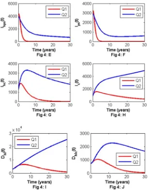
The combination of prevention control strategy, treatment control strategy u2, and screening control strategy u3 are used to optimize objective functional. Results illustrates that

Figure 4. Showing impact of using all control strategies. Figure 4: A - J are time series plot of different population whereQ₁= ≠u₁ 0,u₂≠0,u₃≠0with control and Q2=

(

u1=0,u2=0,u3=0

)

without control.

4. Cost-effectiveness Analysis

Here, Incremental Cost Effectiveness Ratio (ICER) is used to quantify the cost-effectiveness of different strategies. This approach is useful to understand which strategy saves a lot of averted species while spending low cost. This technique is needed to compare more than one competing interventions strategies incrementally, one intervention should be compared with the next less effective alternative [10]. The ICER formula is given by

Difference in intervention cost ICER=

Difference in the total number of infection averted The total number of infection averted is obtained by calculating the difference between the total number of new cases of individuals having HPV infection without control and the total number of new cases of individuals having HPV infection with control.

Table 2. Calculation of ICER after arranging the number of total infections averted in ascending order.

Strategy Total Cost ($) Total infections

Averted ICER

Strategy III $2,480.00 64,637.00 0.0384

Strategy II $2,770.20 75,510.00 0.0266

Strategy I $3,090.00 91,109.00 0.0205

Strategy IV $4,383.30 93,870.00 0.4684

2, 480.50

ICER(Strategy III) 0.0384 64, 637.00

= = ,

2, 770.20 2, 480.50

ICER(Strategy II) 0.0266

75,510.00 64, 637.00

−

= =

− ,

3, 090.00 2, 770.20

ICER(Strategy I) 0.0205

91,109.00 75, 510.00 −

= =

− and

4,383.30 3, 090.00

ICER(Strategy IV) 0.4684

93,870.00 91,109.00 −

= =

− .

is less than ICER of strategy III. Hence strategy III is more costly and less effective than strategy II. Thus, strategy III is omitted and ICER is recalculated.

Table 3. Computation of ICER after dropping strategy III.

Strategy Total Cost($) TotalInfections Averted ICER

Strategy II $2,770.20 75,510.00 0.0367

Strategy I $ 3,090.00 91,109.00 0.0205

Strategy IV $4,383.30 93,870.00 0.4684

Comparing strategy II and strategy I, ICER of strategy I is less than ICER of strategy II. Thus, strategy II is omitted and the ICER is recalculated.

Table 4. Computation of ICER after dropping strategy II.

Strategy Total Cost($) TotalInfections Averted ICER

Strategy I $ 3,090.00 91,109.00 0.0339

Strategy IV $4,383.30 93,870.00 0.4684

By comparing strategy I and strategy IV, ICER of strategy I is less than ICER of strategy IV. Therefore, strategy IV is dropped and strategy I is considered.

Thus, according to Incremental Cost Effectiveness Ratio analysis, the combination of optimal prevention and treatment control strategies is the best way of minimizing cervical cancer among women with or without HIV infection in our community following the combination of all control strategies.

5. Conclusion

This paper designed and analyzed a deterministic model for co-infection of cervical cancer and HIV diseases. The optimal control theory was employed to the main model and analyzed using Potrayagin’s Maximum Principle. The different combination of three optimal control strategies; prevention, screening, and treatment were studied numerically. Also, cost-effectiveness analysis was performed and the following results were obtained

(a)The combination of optimal screening and treatment strategies is not much powerful way of controlling HPV infection and cervical cancer in the community compared with other combination of optimal control strategies as shown in Figure 3. Also, applying the combination of all control strategies (prevention, screening, and treatment) is the best way of minimizing co-infection of cervical cancer and HIV diseases in a community as shown in Figure 4.

(b)In the case of Incremental Cost Effectiveness Ratio analysis, the combination of optimal prevention and treatment strategies is the most cost-effective control to minimize cervical cancer among women with or without HIV infection. The second is the combination of all optimal control strategies; prevention, screening, and treatment. The third is the combination of optimal prevention and screening control strategies.

References

[1] S. E. Hawes, C. W. Critchlow, M. A. Faye Niang, M. B. Diouf, A. Diop, P. Toure, A. Aziz Kasse, B. Dembele, P. Salif Sow, A. M. Coll-Seck, J. M. Kuypers, N. B. Kiviat, H. S. E., C. C. W., F. N. M. A., D. M. B., D. A., T. P., K. A. A., D. B., S. P. S., C.-S. A. M., K. J. M., and K. N. B., “Increased risk of high-grade cervical squamous intraepithelial lesions and invasive cervical cancer among African women with human immunodeficiency virus type 1 and 2 infections,”J. Infect. Dis., 2003, vol. 188, no. 4, pp. 555–563.

[2] S. M. Mbulaiteye, E. T. Katabira, H. Wabinga, D. M. Parkin, P. Virgo, R. Ochai, M. Workneh, A. Coutinho, and E. A. Engels, “Spectrum of cancers among HIV-infected persons in Africa: The Uganda AIDS-Cancer registry match study,” Int. J. Cancer, 2006, vol. 118, no. 4, pp. 985–990.

[3] C. Ng’andwe, J. J. Lowe, P. J. Richards, L. Hause, C. Wood, and P. C. Angeletti, “The distribution of sexually-transmitted human papillomaviruses in HIV positive and negative patients in Zambia, Africa.,” BMC Infect. Dis., 2007, vol. 7, pp. 77. [4] B. Maregere, “Analysis of co-infection of human

immunodeficiency virus with human papillomavirus,” University of KwaZulu-Natal, 2014.

[5] K. O. Okosun and O. D. Makinde, “A co-infection model of malaria and cholera diseases with optimal control,” Math. Biosci., 2014, vol. 258, pp. 19–32.

[6] K. O. Okosun and O. D. Makinde, “Optimal control analysis of malaria in the presence of non-linear incidence rate,” Appl. Comput. Math., 2013, vol. 12, no. 1, pp. 20–32.

[7] K. O. Okosun, O. D. Makinde, and I. Takaidza, “Analysis of recruitment and industrial human resources management for optimal productivity in the presence of the HIV/AIDS epidemic,” J. Biol. Phys., 2013, vol. 39, no. 1, pp. 99–121. [8] S. Lenhart and J. T. Workman, Optimal control applied to

biological models dynamic optimization, 2007.

[9] W. H. Fleming and R. W. Rishel, Deterministic and stochastic optimal control, Springer-Verlag, Berlin Heidelberg New York, 1975.

[10] K. O. Okosun, O. D. Makinde, and I. Takaidza, “Impact of optimal control on the treatment of HIV/AIDS and screening of unaware infectives,” Appl. Math. Model., 2013, vol. 37, no. 6, pp. 3802–3820.

[11] “Tanzania-life expectance at birth.” [Online]. Available:

http://countryeconomy.com/demography/life-expectancy/tanzania. [Accessed: 09-Oct-2016].

[12] S. L. Lee and A. M. Tameru, “A mathematical model of human papillomavirus (HPV) in the united states and its impact on cervical cancer,” J. Cancer, 2012, vol. 3, no. 1, pp. 262–268. [13] R. Federation, S. Africa, and S. Lanka, “Cervical cancer

global crisis card,” Cerv. Cancer Free Coalit., 2013.

[14] “HIV and AIDS in Tanzania,” 2015. [Online]. Available: http://www.avert.org/professionals/hiv-around-world/sub-saharan-africa/tanzania. [Accessed: 09-Oct-2016].