Incremental Algorithms for Hierarchical Classification

Incremental Algorithms for Hierarchical Classification

Nicol`o Cesa-Bianchi [email protected]

Dipartimento di Scienze dell’Informazione Universit`a degli Studi di Milano

via Comelico 39 20135 Milano, Italy

Claudio Gentile [email protected]

Dipartimento di Informatica e Comunicazione Universit`a dell’Insubria

via Mazzini 5 21100 Varese, Italy

Luca Zaniboni [email protected]

Dipartimento di Tecnologie dell’Informazione Universit`a degli Studi di Milano

via Bramante 65 26013 Crema (CR), Italy

Editor: Michael Collins

Abstract

We study the problem of classifying data in a given taxonomy when classifications associated with multiple and/or partial paths are allowed. We introduce a new algorithm that incrementally learns a linear-threshold classifier for each node of the taxonomy. A hierarchical classification is obtained by evaluating the trained node classifiers in a top-down fashion. To evaluate classifiers in our multipath framework, we define a new hierarchical loss function, the H-loss, capturing the intuition that whenever a classification mistake is made on a node of the taxonomy, then no loss should be charged for any additional mistake occurring in the subtree of that node.

Making no assumptions on the mechanism generating the data instances, and assuming a linear noise model for the labels, we bound the H-loss of our on-line algorithm in terms of the H-loss of a reference classifier knowing the true parameters of the label-generating process. We show that, in expectation, the excess cumulative H-loss grows at most logarithmically in the length of the data sequence. Furthermore, our analysis reveals the precise dependence of the rate of convergence on the eigenstructure of the data each node observes.

Our theoretical results are complemented by a number of experiments on texual corpora. In these experiments we show that, after only one epoch of training, our algorithm performs much better than Perceptron-based hierarchical classifiers, and reasonably close to a hierarchical support vector machine.

Keywords: incremental algorithms, online learning, hierarchical classification, second order per-ceptron, support vector machines, regret bound, loss function

1. Introduction

as a taxonomy. That is, we assume that every data instance is labelled with a (possibly empty) set of class nodes and, whenever an instance is labelled with a certain node i, then it is also labelled with all the nodes on the path from the root of the tree where i occurs down to node i. A distinctive feature of our framework is that we also allow multiple-path labellings (instances can be labelled with nodes belonging to more than one path in the forest), and partial-path labellings (instances can be labelled with nodes belonging to a path that does not end on a leaf).

We introduce a new algorithm that incrementally learns a linear-threshold classifier for each node of the taxonomy. A hierarchical classification is then obtained by evaluating the node classi-fiers in a top-down fashion, so that the final labelling is consistent with the taxonomy.

The problem of hierarchical classification, especially of textual information, has been exten-sively investigated in past years (see, e.g., Dumais and Chen, 2000; Dekel et al., 2004, 2005; Gran-itzer, 2003; Hofmann et al., 2003; Koller and Sahami, 1997; McCallum et al., 1998; Mladenic, 1998; Ruiz and Srinivasan, 2002; Sun and Lim, 2001, and references therein). The on-line approach to hierarchical classification, which we analyze here, seems well suited when dealing with scenarios in which new data are produced frequently and in large amounts (e.g., data produced by newsfeeds— considered in this paper, or the speech data considered in Dekel et al., 2005).

An important ingredient in a hierarchical classification problem is the loss function used to evaluate the classifier’s performance. In pattern classification the zero-one loss is traditionally used. In a hierarchical setting this loss would simply count one mistake each time, on a given data instance, the set of class labels output by the hierarchical classifier is not perfectly identical to the set of true labels associated to that instance. Loss functions able to reflect the taxonomy structure have been proposed in the past (e.g., Dekel et al., 2004; Hofmann et al., 2003; Sun and Lim, 2001), but none of these losses works well in our framework where multiple and partial paths are allowed. In this paper we define a new loss function, the H-loss (hierarchical loss), whose simple definition captures the following intuition: “if a mistake is made at node i of the taxonomy, then further mistakes made in the subtree rooted at i are unimportant”. In other words, we do not require the algorithm be able to make fine-grained distinctions on tasks where it is unable to make coarse-grained ones.

For example, if an algorithm failed to label a document with the classSPORTS, then the algorithm

should not be charged more loss because it also failed to label the same document with the subclass

SOCCERand the sub-subclassCHAMPIONS LEAGUE.

We bound the theoretical performance of our algorithm using the H-loss. In our analysis, we make no assumptions on the mechanism generating the data instances; that is, we bound the H-loss of the algorithm for any arbitrary sequence of data instances. The hierarchical labellings associated to the instances, instead, are assumed to be independently generated according to a parametric stochastic process defined on the taxonomy.

in the forest. In general, the overall cumulative regret is seen to grow at most logarithmically in the length T of the data sequence.

From the theoretical point of view, the novelty of this line of research is twofold:

1. The use of hierarchically trained linear-threshold classifiers is common to several of the pre-vious approaches to hierarchical classification (e.g., Dumais and Chen, 2000; Dekel et al., 2004, 2005; Granitzer, 2003; Hofmann et al., 2003; Koller and Sahami, 1997; McCallum et al., 1998; Mladenic, 1998; Ruiz and Srinivasan, 2002; Sun and Lim, 2001). However, to our knowledge, this research is the first one to provide a rigorous performance analysis of hi-erarchical classification algorithms in the presence of multiple and partial path classifications.

2. The core of our analysis is a local cumulative regret bound showing that the instantaneous

regret of each node classifier vanishes at a rate 1/T . The precise dependence of the rate

of convergence on the eigenstructure of the data each node observes is a major contribution of this paper. This turns out to be similar in spirit to early (and classical) work in least-squares linear regression (e.g., Lai et al., 1979; Lai and Wei, 1982). But unlike these previous investigations, our analysis is not asymptotic in nature and studies a specific classification setting, instead of a regression one.

To support our theoretical findings we also describe some experiments concerning a more practical variant of the algorithm we actually analyze. These experiments use large corpora of textual data on which we test different batch and incremental classifiers. The experiments show that our on-line algorithm performs significantly better than Perceptron-based hierarchical classifiers. Furthermore, after only one epoch of training, our algorithm achieves a performance close to that of a hierar-chical support vector machine, the popular batch learning algorithm for which, to the best of our knowledge, no theoretical performance bounds are known in hierarchical classification frameworks. The paper is organized as follows. Section 2 defines the notation used throughout the paper. In Section 3 we introduce the H-loss function. Our hierarchical algorithm is described in Section 4. In Section 5 and 6 we define the data model, the learning model, and our theoretical performance measure: the cumulative regret. The analysis of our algorithm is carried out in Section 7, while in Section 8 we report on the experiments. Finally, in Section 9 we summarize our results and mention a few open questions.

2. Notation

We assume data elements are encoded as unit-norm vectors x_∈Rd, which we callinstances. A

multilabel for an instance x is any subset of the set_{1, . . . ,N} of all labels, including the empty set. We represent the multilabel of x with a vector v= (v1, . . . ,vN)∈ {0,1}N, where i∈ {1, . . . ,N}

belongs to the multilabel of x if and only if vi=1.

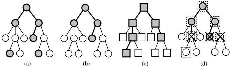
Ataxonomy G is a forest whose trees are defined over the set of labels. A multilabel v_{∈ {}0,1_}N

is said torespect a taxonomy G if and only if v is the union of one or more paths in G, where each

path starts from a root but need not terminate on a leaf, see Figure 1. We assume the data-generating

mechanism produces examples(x,v)such that v respects some fixed underlying taxonomy G with

N nodes (see Section 5). The set of roots in G is denoted byROOT(G). We usePAR(i)to denote the

2

2 33

5

5

4

6

6

7

7 ₈₈ 99

10 11

1 1 P(V1_|x)

P(V11_|V8,x)

P(V4_|V3,x)

Figure 1: A forest made of two disjoint trees. The nodes are tagged with the name of the

la-bels, so that in this case N = 11. According to our definition, the multilabel v=

(1,1,1,0,0,1,0,1,0,1,0) respects this taxonomy (since it is the union of paths 1_→2, 1_→3 and 6_→8_→10), while the multilabel v= (1,1,0,1,0,0,0,0,0,0,0) does not,

since 1_→2_→4 is not a path in the forest. Associated with each node i is a_{0,1_}

-valued random variable Vi distributed according to a conditional probability function

P(Vi|VPAR(i),x)—see Section 5.

We denote by_{φ_}the Bernoulli random variable which is 1 if and only if predicateφis true. In our analysis, we repeatedly use simple facts such as_{φ_∨ψ_}=_{φ_}+_{ψ_{∧ ¬}φ_{} ≤ {}φ_}+_{ψ_}and {φ}=_{φ_∧ψ_}+_{φ_{∧ ¬}ψ_{} ≤ {}φ_∧ψ_}+_{¬ψ_}, whereψis another predicate.

3. The H-Loss

Two very simple loss functions, measuring the discrepancy between the prediction multilabel_by=

(y1_b, . . . ,_byN)and the true multilabel v= (v1, . . . ,vN), are the zero-one loss`0/1(by,v) ={∃i :byi6=vi}

and the symmetric difference loss`_∆(_by,v) =_{by16=v1}+. . .+{ybN6=vN}. Note that the definition of

these losses is based on the set_{1, . . . ,N_}of labels without any additional structure. A loss function that takes into account a taxonomical structure defined over the set of labels is

`H(by,v) = N

∑

i=1

{ybi6=vi∧ybj=vj, j∈ANC(i)}.

This loss, which we call H-loss (hierarchical loss), can also be defined as follows: all paths in G from a root down to a leaf are examined and, whenever a node i is encountered such thatbyi 6=vi,

then 1 is added to the loss, while all the loss contributions in the subtree rooted at i are discarded. Note that, with this definition,`0/1≤`H≤`∆. A graphical representation of the H-loss and related

concepts is given in Figure 2.

In the next lemma we show an important (and intuitive) property of the H-loss: when the mul-tilabel v to be predicted respects a taxonomy G then there is no loss of generality in restricting to predictions which respect G. Formally, given a multilabel_by_{∈ {}0,1_}N_{, we define the G-truncation}

of_by as the multilabel_by0= (y_b0₁, . . . ,y_b0_N)_{∈ {}0,1_}N where, for each i=1, . . . ,N,y_b0_i=1 if and only if b

yi=1 andbyj =1 for all j∈ANC(i). Note that the G-truncation of any multilabel always respects

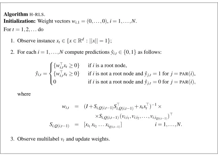
(a) (b) (c) (d)

Figure 2: A one-tree forest (repeated four times). Each node corresponds to a class in the taxonomy G, hence in this case N=12. Gray nodes are included in the multilabel under consid-eration, white nodes are not. (a) A generic multilabel which does not respect G; (b) its G-truncation. (c) A second multilabel that respects G. (d) Superposition of multilabel (b) on multilabel (c): Only the checked nodes contribute to the H-loss between (b) and (c). Hence the H-loss between multilabel (b) and multilabel (c) is 3. Here the zero-one loss between (b) and (c) is 1, while the symmetric difference loss equals 4.

Lemma 1 Let G be a taxonomy, v,_by_{∈ {}0,1_}N be two multilabels such that v respects G, and_by0 be the G-truncation of_by. Then

`H(by0,v)≤`H(by,v).

Proof. Since `H(by0,v) =∑Ni=1{yb0i6=vi∧by0j=vj,j∈ANC(i)} and`H(by,v) =∑Ni=1{byi6=vi∧byj=

vj, j∈ANC(i)}, it suffices to show that, for each i=1, . . . ,N,byi06=viandby0j=vj for all j∈ANC(i)

impliesybi6=viandbyj=vj for all j∈ANC(i).

Pick some i and supposey_b0_i6=vi andby0j=vj for all j∈ANC(i). Now supposeby0j=0 (and thus

vj=0) for some j∈ANC(i). Then vi=0 since v respects G. But this impliesby0i=1, contradicting

the fact that the G-truncation_by0 respects G. Therefore, it must be the case that_by0_j =vj =1 for all

j_∈ANC(i). Hence the G-truncation ofby left each node j∈ANC(i)unchanged, implyingbyj=vjfor

all j_∈ANC(i). But, since the G-truncation of_by does not change the value of a node i whose ancestors j are such thaty_bj=1, this also impliesbyi=by0i. Thereforebyi6=viand the proof is concluded.

4. A New Hierarchical Learning Algorithm

In this section we describe our on-line algorithm for hierarchical classification. Its theoretical per-formance is analyzed in Section 7.

The on-line learning model we consider is the following. In the generic time step t =1,2, . . .

instance xt is revealed to the algorithm which outputs the predictionbyt = (yˆ1,t, . . . ,yˆN,t)∈ {0,1}N.

This is viewed as a guess for the multilabel vt = (v1,t,v2,t, . . . ,vN,t) associated with the current

instance xt. After each prediction, the algorithm observes the true multilabel vt and adjusts its

parameters for the next prediction.

Our algorithm computes ˆy1,t, . . . ,yˆN,t using N linear-threshold classifiers, one for each node in

AlgorithmH-RLS.

Initialization: Weight vectors wi,1= (0, . . . ,0), i=1, . . . ,N. For t=1,2, . . .do

1. Observe instance xt∈ {x∈Rd :||x||=1};

2. For each i=1, . . . ,N compute predictions ˆyi,t ∈ {0,1}as follows:

ˆ yi,t =

  

 

{w>_i,txt≥0} if i is a root node,

{w>_i,txt≥0} if i is not a root node and ˆyj,t =1 for j=PAR(i),

0 if i is not a root node and ˆyj,t =0 for j=PAR(i),

where

wi,t = (I+Si,Q(i,t−1)Si>,Q(i,t₋1)+xtx>t )−1×

×Si,Q(i,t−1)(vi,i1,vi,i2, . . . ,vi,iQ(i,t−1))> S_i,Q(i,t−1) = [xi1xi2. . .xiQ(i,t−1)] i=1, . . . ,N.

3. Observe multilabel vt and update weights.

Figure 3: The hierarchical learning algorithmH-RLS.

0 then all of its descendants are labelled 0. Note that this evaluation scheme can only generate

multilabels that respect the underlying taxonomy.

Let w1, . . . ,wN be the weight vectors defining the linear-threshold classifiers used by the

algo-rithm. A feature of the learning process, which is also important for its theoretical analysis, is that the classifier at node i is only trained on the examples that are positive for its parent node. In other words, wiis considered for update only on those instances xt such that vPAR(i),t =1.

Let Q(i,t)denote the number of times theparent of node i observes a positive label up to time t, i.e., Q(i,t) =_|{1_≤s_≤t : vPAR(i),s=1}|. The weight vector wi,t stored at time t in node i is a

(conditional) regularized least squares estimator given by

wi,t=

I+Si,Q(i,t−1)Si>,Q(i,t₋1)+xtx>t

₋1

Si,Q(i,t−1)(vi,i1, . . . ,vi,iQ(i,t−1))>, (1) where I is the d_×d identity matrix, Si,Q(i,t−1)is the d×Q(i,t−1)matrix whose columns are the instances xi1, . . . ,xiQ(i,t−1), and(vi,i1, . . . ,vi,iQ(i,t−1))>is the Q(i,t−1)-dimensional (column) vector of the corresponding labels observed by node i.

The estimator in (1) is a slight variant of the regularized least squares estimator for

classifi-cation (Cesa-Bianchi et al., 2002; Rifkin et al., 2003) where we include the current instance xt in

the computation of wi,t (see, e.g., Azoury and Warmuth, 2001; Vovk, 2001, for analyses of

dual variable formulations of the algorithm are extensively discussed by Cesa-Bianchi et al. (2002) and Rifkin et al. (2003).

The pseudocode of our algorithm, which we callH-RLS(Hierarchical Regularized Least Squares)

is given in Figure 3.

5. A Stochastic Model for Generating Labels

While no assumptions are made on the mechanism generating the sequence x1,x2, . . .of instances, we base our analysis on the following stochastic model for generating the multilabel associated to an instance xt.

A probability distribution fGover the set of multilabels is associated to a taxonomy G as

fol-lows. Each node i of G is tagged with a_{0,1_}-valued random variable Vi distributed according to

a conditional probability functionP(Vi|VPAR(i),x). To model the dependency between the labels of nodes i and j=PAR(i)we assume

P(Vi=1|Vj=0,x) =0 (2)

for all nonroot nodes i and all instances x. For example, in the taxonomy of Figure 1 we have P(V4=1|V3=0,x) =0 for all x∈Rd. The quantity

fG(v|x) = N

∏

i=1

P(Vi=vi|Vj=vj,j=PAR(i),x)

thus defines a joint probability distribution on V1, . . . ,VNconditioned on x being the current instance.

This joint distribution puts zero probability on all multilabels v_{∈ {}0,1_}N which do not respect G. Through fG we specify an i.i.d. process{V1,V2, . . .}as follows. We assume that an arbitrary and unknown sequence of instance vectors x1,x2, . . .is fixed in advance, where kxtk=1 for all

t. The multilabel Vt is distributed according to the joint distribution fG(· |xt). We call each pair (xt,vt), where vt is a realization of Vt, anexample.

Let us now introduce a parametric model for fG. With each node i in the taxonomy, we associate

a unit-norm weight vector ui∈Rd. Then, we define the conditional probabilities for a nonroot node

i with parent j as follows:

P(Vi=1|Vj=1,x) =

1+u>_i x

2 . (3)

If i is a root node, the above simplifies to

P(Vi=1|x) =

1+u>_i x

2 .

Our choice of a linear model for Bernoulli random variables, as opposed to a more standard log-linear model, is mainly motivated by our intention of proving regret bounds with no assumptions on the way the sequence of instances is generated. Indeed, we are not aware of any analysis of logistic regression holding in a similar classification setup.

6. Regret and the Reference Classifier

Assuming the stochastic model described in Section 5, we compare the performance of our algo-rithm to the performance of the fixed hierarchical classifier built on the true parameters u1, . . . ,uN

governing the label-generating process. This reference hierarchical classifier has the same form as the classifiers generated byH-RLS. More precisely, let the multilabel y= (y1, . . . ,yN)for an instance

x be computed as follows:

yi=

    

{u>_i x_≥0_} if i is a root node,

{u>_i x_≥0_} if i is not a root and yj=1 for j=PAR(i),

0 if i is not a root and yj=0 for j=PAR(i).

(4)

To evaluate our algorithm against the reference hierarchical classifier defined in (4), we use the

cumulative regret. Given any loss function `(such as one of the three defined in Section 3), we

define the (instantaneous) regret of a classifier assigning label_by_t to instance xt as

E`(<sub>b</sub>y<sub>t</sub>,Vt)−E`(yt,Vt),

where y_t is the multilabel assigned by classifier (4), and the expectation is with respect the random draw of Vt(as specified in Section 5). We measure the performance ofH-RLSthrough its cumulative

regret on a sequence of T examples:

T

∑

t=1

E`(<sub>b</sub>y<sub>t</sub>,Vt)−E`(yt,Vt)

. (5)

The regret bound we prove in Section 7 holds when`=`H, and is shown to depend on the interaction

between the spectral structure of the data generating process and the structure of the taxonomy on which the process is applied.

7. Analysis

We now prove a bound on the cumulative regret ofH-RLSwith respect to the H-loss function`H.

Our analysis hinges on proving that for any node i, the estimated margin w>_i,txt is an asymptotically

unbiased estimator of the true margin u>_i xt, and then on using known large deviation arguments to

obtain the stated bound. For this purpose, we bound the variance of the margin estimator at each node and prove a bound on the rate at which the bias vanishes.

Theorem 2 Consider a taxonomy G with N nodes. Pick any set of model parameters u1, . . . ,uN∈

Rdsuch that_kuik=1 for i=1, . . . ,N, and pick any sequence of instance vectors x1,x2, . . .∈Rdsuch that_kxtk=1 for all t. Then the cumulative regret of the H-RLSalgorithm (described in Figure 3)

satisfies, for each T _≥1,

T

∑

t=1

E`H(byt,Vt)−E`H(yt,Vt)

≤16(1+1/e) N

∑

i=1 Ci

∆2

i

E "

d

∑

j=1

log(1+λi,j)

#

,

where

∆i,t=u>i xt, ∆2i = min t=1,...,T∆

2

i,t, Ci=|SUB(i)|,

Before delving into the proof, it is worth making a few comments.

Remark 3 Since H-RLS can be cast in dual variables, we can run it in any reproducing kernel Hilbert space (e.g., Sch¨olkopf and Smola, 2002). The regret bound contained in Theorem 2 remains true once we observe that the nonzero eigenvalues of S_i,Q(i,T)S>_i,Q(i,T) coincide with the nonzero eigenvalues of the Gram matrix S>_i,Q(i,T)Si,Q(i,T), and we replace the sum over all input dimensions d with the sum over the (at most T ) nonzero eigenvalues of S>_i,Q(i,T)Si,Q(i,T). We refer the reader to the work by Cesa-Bianchi et al. (2002) for additional details.

Remark 4 It is important to emphasize the interplay between the taxonomy structure and the process generating the examples, as expressed by the above regret bound. Recall that we de-note byλi,1, . . . ,λi,d the eigenvalues of matrix Si,Q(i,T)S>_i,Q(i,T). From the previous remark we have ∑d

j=1λi,j=trace S>_i,Q(i,T)Si,Q(i,T)

=Q(i,T)since_kxtk=1∀t, and

d

∑

j=1

log(1+λi,j)≤max

(

d

∑

j=1

log(1+µj) : d

∑

j=1

µj=Q(i,T)

)

=d log

1+Q(i,T)

d

.

Moreover, Q(i,T)is the sum of T Bernoulli random variables, where the t-th variable takes value

1 when the parent of the i-th node in the taxonomy observes label VPAR(i),t =1 at time t. The

probability of this event clearly equals

∏

j∈ANC(i)

1+∆j,t

2 . Thus E " d

∑

log(1+λi,j)

#

≤ dE

log

1+Q(i,T)

d

(6)

≤ d log

1+EQ(i,T)

d

(from Jensen’s inequality)

= d log  1+∑

T

t=1∏j∈ANC(i) _1+∆

j,t

2

d



. (7)

Bound (6) is obviously a log T cumulative regret bound, since Q(i,T)_≤T anyway. It is important, however, to see how the regret bound depends on the taxonomy structure. Let us focus on (7). If i is a root node thenEQ(i,T) =Q(i,T) =T (since a root node observes all labels). As we descend

along a path, EQ(i,T) tends to decrease with a rate depending on the margins achieved by the

ancestors of node i. Bound (7) thus makes explicit the contribution of node i to the overall regret. If i is a root node, then its contribution to the overall regret is roughly log T . On the other hand, the deeper is node i within the taxonomy the smaller is the contribution of node i to the overall regret. A very deep leaf node observes a possibly small subset of the instances, but it is also required to produce only a small subset of linear-threshold predictions, i.e., the associated weight vector wi,t

Remark 5 Nothing prevents us from generalizing the H-loss by associating fixed cost coefficients to each taxonomy node:

`H(by,v) = N

∑

i=1

ci{byi6=vi∧byj=vj,j∈ANC(i)},

where the cost coefficients ci are positive real numbers. It is straightforward to see that with this

definition of H-loss, the statement of Theorem 2 still holds, once we generalize the regret factors Cias Ci=∑k∈SUB(i)ck. Note that this would involve changes neither in our learning algorithm nor

in our reference predictor. In fact, we are measuring regret against a reference predictor that is not Bayes optimal for the data model at hand. This is not immediate to see when the cost coefficients ci

defining the H-loss are all set to 1 but, as we mentioned, it is generally evinced by the fact that both the reference predictor (4) and our learning algorithm do not depend on the ci.

Remark 6 From the proof of Theorem 2 below, the reader can see that there are several ways one can improve the bounds. In fact, we made no special effort to minimize the main constant 16(1+1/e) and, in general, we disregarded quite a lot of constant factors throughout. Moreover, though we decided to cast the bounds in terms of the worst-case margin∆2_i =mint=1,...,T∆2i,t, it is

straighforward to modify the proof to obtain a bound depending on some sort of average squared margin. Since this sharper bound would hide the clean dependence on the eigenstructure of the data, we decided not to pursue this optimization any further.

We are now ready to prove Theorem 2.

Proof of Theorem 2. We fix a node i and upper bound its contribution to the total instantaneous regret. Since for any four predicatesφ,ψ,χ,ζwe have_{φ_∧ψ_{} − {}χ_∧ζ_{} ≤ {}φ_∧ψ_{∧ ¬}χ_}+_{φ_∧ψ_∧

χ∧ ¬ζ}, we see that

{byi,t 6=Vi,t,∀j∈ANC(i) :ybj,t=Vj,t} − {yi,t6=Vi,t,∀j∈ANC(i) : yj,t =Vj,t}

≤byi,t6=Vi,t,yi,t=Vi,t,∀j∈ANC(i) :byj,t=Vj,t (8) +_byi,t 6=Vi,t,yi,t6=Vi,t,∀j∈ANC(i) :byj,t =Vj,t,∃j∈ANC(i): yj,t 6=Vj,t . (9)

We bound the two terms (8) and (9) separately. We can write:

(8) =_{byi,t 6=Vi,t,yi,t =Vi,t,∀j∈ANC(i) :ybj,t =Vj,t=1}

(since_byj,t=Vj,t =0 for some ancestor j impliesbyi,t =Vi,t=0)

≤ {byi,t 6=yi,t,

K

where we have introduced the short-hand

K

have

(9) =_{y_bi,t6=Vi,t,yi,t 6=Vi,t,∀j∈ANC(i) :ybj,t=Vj,t=1,∃j∈ANC(i) : yj,t6=Vj,t} =_{y_bi,t6=Vi,t,yi,t =6 Vi,t,∀j∈ANC(i) :ybj,t=Vj,t=1,∃j∈ANC(i) :ybj,t6=yj,t}

≤ {∃j_∈ANC(i) :byj,t6=yj,t,

K

≤

∑

j∈ANC(i)

{ybj,t 6=yj,t,

K

≤

∑

j∈ANC(i)

where the last inequality holds because

K

K

`H(byt,Vt)−`H(yt,Vt)

= N

∑

i=1

{byi,t 6=Vi,t,∀j∈ANC(i) :ybj,t=Vj,t} − {yi,t6=Vi,t,∀j∈ANC(i) : yj,t =Vj,t}

≤

N

∑

i=1j_∈ANC

∑

{byj,t6=yj,t,

K

= N

∑

i=1

{byi,t 6=yi,t,

K

∑

1

= N

∑

i=1

Ci{ybi,t6=yi,t,

K

We then take expectations and sum over t:

T

∑

t=1

E`H(byt,Vt)−E`H(yt,Vt)

≤

T

∑

t=1

N

∑

i=1

CiP(ybi,t=6 yi,t,

K

= N

∑

i=1 Ci

T

∑

t=1

P(y_bi,t6=yi,t,

K

Equation (10) is a conveniently simple upper bound on the cumulative regret. This allows us to focus on bounding from above the one-node cumulative expectation∑_tT₌₁P(_byi,t 6=yi,t,

K

For brevity, in the rest of this proof we use the notations∆i,t =u>i xt (the target margin on xt)

and∆bi,t=w>i,txt (the algorithm margin on xt). As we said earlier, our argument centers on proving

that for any node i,∆bi,t is an asymptotically unbiased estimator of∆i,t, and then on using known

large deviation techniques to obtain the stated bound. For this purpose, we need to study both the conditional bias and the conditional variance ofb∆i,t.

Recall Figure 3. Since the sequence x1,x2, . . . is fixed, the multilabel vectors Vt are

statisti-cally independent. Also, for any t =1,2, . . .and for any node i with parent j, the child’s labels Vi,i1, . . . ,Vi,iQ(i,t−1) are independent when conditioned on the parent’s labels Vj,1, . . . ,Vj,t−1. We use the notation

Ei,t=E[· |Vj,1, . . . ,Vj,t−1].

By definition of our parametric model (3) we haveEi,t[(Vi,i1, . . . ,Vi,iQ(i,t−1))>] =S>i,Q(i,t−1)ui.

Recall-ing the definition (1) of wi,t, this implies (for conciseness we write Q instead of Q(i,t−1))

Ei,t[∆bi,t] =u>i Si,QS>i,Q(I+Si,QS>i,Q+xtx>t )−1xt .

Note that

∆i,t=Ei,t[∆bi,t] +u>i (I+xtxt>)(I+Si,QS>i,Q+xtx>t )−1xt =Ei,t[b∆i,t] +Bi,t,

where Bi,t =u>i (I+xtx>t )(I+Si,QS>i,Q+xtxt>)−1xt is the conditional bias of wi,t. It is useful to

introduce the short-hand notation

Also, in order to stress the dependence1of ri,t on Q=Q(i,t−1), we denote it by ri,t,Q.

The conditional bias is bounded in the following lemma (proven in the appendix).

Lemma 7 With the notation introduced so far, we have

Bi,t ≤√ri,t,Q+|∆i,t|ri,t,Q.

As far as the conditional variance ofb∆i,t is concerned, from Figure 3 we see that

b ∆i,t=

Q

∑

k=1

Vi,ikZi,t,k,

where

Z>_i,t = (Zi,t,1, . . . ,Zi,t,Q) =S>i,Q

I+Si,QSi>,Q+xtxt>

−1

xt . (11)

The next lemma (proven in the appendix) handles the conditional variance_kZi,tk2.

Lemma 8 With the notation introduced so far, we have

kZi,tk2≤ri,t,Q.

Armed with these two lemmas, we proceed through our large deviation argument. We can write

{yˆi,t 6=yi,t,

K

≤ n∆bi,t∆i,t≤0,

K

o

≤ n|b∆i,t−∆i,t| ≥ |∆i,t|,

K

o

≤ n|b∆i,t+Bi,t−∆i,t| ≥ |∆i,t| − |Bi,t|,

K

o

≤ n|b∆i,t+Bi,t−∆i,t| ≥ |∆i,t|/2,

K

o

+_{|Bi,t| ≥ |∆i,t|/2,

K

We can further bound the second term of (12) by using Lemma 7. We obtain

n

|Bi,t| ≥ |∆i,t|/2,

K

o

≤ {√ri,t,Q+|∆i,t|ri,t,Q≥ |∆i,t|/2,

K

≤ ri,t,Q≥ |∆i,t|2/16∨ri,t,Q≥1/4,

K

K

1. As it turns out, many of the quantities appearing in the present proof, including the bias term Bi,t and the variance

vector Zi,tdefined later on, are algorithm-dependent, hence they do actually depend on Q=Q(i,t−1). However, this

dependence is made notationally explicit only for the quantity ri,t=ri,t,Qsince, we believe, this specific dependence

the equality following from the fact that |∆i,t|2/16≤1/16<1/4. We plug back into (12), take

expectations, and sum over t. We have

E "_T

∑

t=1

{yˆi,t6=yi,t,

K

# ≤ E "_T

∑

|b∆i,t+Bi,t−∆i,t| ≥ |∆i,t|/2,

K

o

+ri,t,Q≥ |∆i,t|2/16,

K

#

= E

"_T

∑

t=1

{

K

n

|∆bi,t+Bi,t−∆i,t| ≥ |∆i,t|/2

o# (13) +E "_T

∑

ri,t,Q≥ |∆i,t|2/16,

K

#

, (14)

where in (13) we used the fact that

K

We now bound the two expectations (13) and (14) separately. Let j=PAR(i). To bound the

first expectation, we exploit the fact that Vi,i1, . . . ,Vi,iQ are independent under the law Pi,t =P · |

Vj,1, . . . ,Vj,t−1

, and Zi,t,1, . . . ,Zi,t,Q defined in (11) are determined given Vj,1, . . . ,Vj,t−1. Hence, we can apply Chernoff-Hoeffding inequality (Hoeffding, 1963) to the sumb∆i,t =Vi,i1Zi,t,1+. . .+

Vi,iQZi,t,Q of independent random variables, where Ei,t[b∆i,t] =∆i,t−Bi,t and (Vi,i1Zi,t,1)

2_{+. . .+}

(Vi,iQZi,t,Q)

2_≤r

i,t,Qby Lemma 8. Recalling that∆2i =mint=1,...,T∆2i,t, we can write T

∑

t=1

{

K

|b∆i,t+Bi,t−∆i,t| ≥ |∆i,t|/2

≤2

T

∑

t=1

{

K

− ∆ 2

i

8 ri,t,Q

.

This quantity can be further upper bounded using the following lemma (proven in the appendix).

Lemma 9 Letα,M be positive constants. Then

max (

n

∑

t=1

e−α/at _{: a}

1≥0, . . . ,an≥0, n

∑

t=1 at=M

)

≤ M eα .

If we let

Mi= T

∑

t=1

{

K

∑

ri,t,Q

we immediately see that Lemma 9 implies

T

∑

t=1

{

K

− ∆ 2

i

8 ri,t,Q

=

∑

t :{Ki,t}=1

exp

− ∆ 2

i

8 ri,t,Q

≤ 8 e∆2

i

Mi.

Therefore,

(13)_≤ 16

To bound (14) we can argue as follows (note that, by definition, ri,t,Q≥0, since it is the value of a

quadratic form with a positive definite matrix):

Mi = T

∑

t=1

{

K

= T

∑

t=1

{ri,t,Q≥∆2i/16,

K

∑

t=1

{ri,t,Q<∆2i/16,

K

≥

T

∑

t=1

{ri,t,Q≥∆2i/16,

K

Hence

(14) =E "

T

∑

t=1

{ri,t,Q≥∆2i/16,

K

#

≤ 16_∆2

i

EMi.

We have thus obtained the following bound

T

∑

t=1

P(yˆi,t6=yi,t,

K

16(1+1/e)

∆2

i

EMi.

To conclude, we need to upper boundEMi. Observe that Miis a sum only over time steps t such that

{

K

we would like to relate Mito the spectral structure of the data correlation matrices Si,Q(i,T)S>i,Q(i,T), we can proceed through the standard upper bounding argument (Azoury and Warmuth, 2001; Cesa-Bianchi et al., 2002) given below.

Mi = T

∑

t=1

{

K

= T

∑

t=1

1₋det

(I+Si,Q(i,t−1)S>i,Q(i,t−1)) det(I+Si,Q(i,t)S>_i,Q(i,t))

!

(using Lemma 2, part 1, in Lai and Wei, 1982)

≤

T

∑

t=1

log det(I+Si,Q(i,t)S >

i,Q(i,t)) det(I+Si,Q(i,t₋1)S>i,Q(i,t−1))

(since 1₋x_{≤ −}log x for all x>0)

= logdet(I+Si,Q(i,T)S >

i,Q(i,T)) det(I)

= d

∑

j=1

log(1+λi,j).

Putting together as in (10) concludes the proof.

Our analysis of Theorem 2 is similar in spirit to the work of Lai et al. (1979) on least-squares regression. In particular, they also assume the sequence x1,x2, . . .be arbitrary while the real-valued labels yt are defined as yt =u>xt+εt, whereεt are i.i.d. random variables with finite variance.

loss, following the same lines as the proof of Theorem 2. As far as the symmetric difference loss

`∆ is concerned, a regret analysis might be obtained through a method we developed in earlier

work (Cesa-Bianchi et al., 2004). As a matter of fact, the analysis by Cesa-Bianchi et al. (2004) rests on several side assumptions about the way data x1, . . . ,xT are generated. We have been unable

to apply the theoretical arguments employed in the present paper to`∆. In any case, since these two loss functions are unable to capture the hierarchical nature of our classification problem, we believe the resulting bounds are less relevant to this paper.

8. Experimental Results

We tested the empirical performance of our on-line algorithm on data sets extracted from two pop-ular corpora of free-text documents. The first data set consists of the first (in chronological order)

100,000 newswire stories from the Reuters Corpus Volume 1 (Reuters, 2000). The associated

tax-onomy of labels, which are the document topics, contains 101 nodes organized in a forest of 4 trees. The forest is shallow: the longest path has length 3 and the distribution of nodes, sorted by increasing path length, is_{0.04,0.53,0.42,0.01_}. The average number of paths in the multilabel

of an instance is 1.5. For this data set we used the bag-of-words vectorization performed by Xerox

Research Center Europe within the EC project KerMIT (see Cesa-Bianchi et al., 2003, for details).

The 100,000 documents were divided into 5 equally sized groups of chronologically consecutive

documents. We then used each adjacent pair of groups as training and test set for an experiment (here the fifth and first group are considered adjacent), and then averaged the test set performance over the 5 experiments.

The second data set includes the documents classified in the nodes of the subtree rooted in “Quality of Health Care” (MeSH code N05.715) of the OHSUMED corpus of medical abstracts (Hersh, 1994). Since OHSUMED is not quite a tree but a directed acyclic graph, and since the H-loss is defined for trees only, we removed from this OHSUMED fragment the few nodes that did not have a unique path to the root. This produced a hierarchy with 94 classes and a data set with

55,503 documents. The choice of this specific subtree was motivated by its structure only; in

particular: the subtree depth is 4, the distribution of nodes (sorted by increasing path length) is {0.26,0.37,0.22,0.12,0.03_}, and there is a reasonable number of partial and multiple path

multil-abels (the average number of paths per instance is 1.53). The vectorization of the documents was

carried out similarly to RCV1. After tokenization, we removed all stopwords and also those words that did not occur at least 3 times in the corpus. Then, we vectorized the documents using the BOW library (McCallum, 2004) with a log(1+TF)log(IDF)encoding. We ran 5 experiments by randomly

splitting the corpus in a training set of 40,000 documents and a test set of 15,503 documents. Test set performances are averages over these 5 experiments. In the training set we kept more docu-ments than in the RCV1 splits since the OHSUMED corpus turned out to be a harder classification problem than RCV1. In both data sets instances have been normalized to unit length.

Since the space complexity of H-RLS grows linearly with training time, due to the need of

storing each training instance in the matrices Si,t —see (1), we had to make some modifications

to the algorithm in order to be able to carry out experiments on data sets of this size. For this purpose, we have developedSH-RLS, a space-efficient variant ofH-RLSthat we used in all of our experiments.

version of Vapnik’s support vector machine (see, e.g., Vapnik, 1998; Sch¨olkopf and Smola, 2002),

and a flat version of SH-RLS. Note that support vector machines are not trained incrementally;

we include them in our pool of baseline algorithms to show that on-line learners, processing each training example only once, can have a performance level close to that of batch learners.

Note also that, unlike our theoretical analysis based on cumulative regret, in the experiments we distinguish a training phase, where the hierarchical classifiers are built, and a test phase, where the performance of the hierarchical classifiers obtained in the training phase is measured on fresh data. This allows us to use a single measure, the test error, to compare both batch and incremental learners.

The first algorithm we consider, H-PERC, is a simple hierarchical version of the Perceptron.

Its functioning differs fromH-RLSdescribed in Figure 3 only in the way weights are updated. In

particular, H-PERC learns a hierarchical classifier by training a linear-threshold classifier at each node via the Perceptron algorithm. At the beginning, the weight vector of each node classifier is set to the zero vector, wi,1= (0, . . . ,0)for i=1, . . . ,N. Upon receiving an example(xt,vt),H-PERC

considers for an update only those classifiers sitting at nodes i satisfying either i_∈ROOT(G) or vPAR(i),t =1. If{w>i,txt≥0} 6=vi,t for such a node i, then the weight vector wi,t is updated using the

Perceptron rule wi,t+1=wi,t+vi,txt; on the other hand, if{w>i,txt ≥0}=vi,t, then wi,t+1=wi,t (no

update takes place at node i).

During the test phase,H-PERCcomputes the multilabel_by= (_by1, . . . ,_byN)of a test instance x using

the same top-down process described in Figure 3,

b yi=

  

 

{w>_i x_≥0_} if i is a root node,

{w>_i x_≥0_} if i is not a root node and ˆyj=1 for j=PAR(i),

0 if i is not a root node and ˆyj=0 for j=PAR(i).

(15)

The second incremental algorithm considered is SH-RLS, our sparse variant of H-RLS. The two

algorithms, H-RLS and SH-RLSoperate in the same way (see Figure 3) with the only difference

thatSH-RLSperforms fewer updates in the training phase. In particular, given a training example

(xt,vt), both algorithms consider for an update only those classifiers sitting at nodes i satisfying

either i_∈ROOT(G) or vPAR(i),t =1. However, whereas H-RLS would update the weight wi,t of

all such nodes i,SH-RLSalso requires the margin condition |w>_i,txt| ≤

p

(5 lnt)/Ni,t, where Ni,t is

the number of instances stored at node i up to time t₋1. The choice of the margin threshold

p

(5 lnt)/Ni,t is motivated by Cesa-Bianchi et al. (2003) via a large deviation analysis.

We also tested a hierarchical version of SVM (denoted by H-SVM) in which each node is an

SVM classifier trained using a batch version of our hierarchical learning protocol. More precisely, each node i was trained only on those examples (xt,vt) such that vPAR(i),t =1. The resulting set

of linear-threshold functions was then evaluated on the test set using the hierarchical classification

scheme (15). We tried both the C andνparametrizations (Sch¨olkopf et al., 2000) for SVM and found

the setting C=1 to work best2for our data (recall that all instances xt are normalized,kxtk=1).

We finally tested the “flat” variants of H-PERC, SH-RLSandH-SVM, denoted byPERC, S-RLS

andSVM, respectively. In these variants, each node is trained and evaluated independently of the

others, disregarding all taxonomical information. All SVM experiments were carried out using the libSVM implementation (Chang and Lin, 2004) and all the algorithms ran with a linear kernel. The

RCV1

Algorithm zero-one loss uniform H-loss ∆-loss

PERC 0.702(_±0.045) 1.196(_±0.127) 1.695(_±0.182)

H-PERC 0.655(±0.040) 1.224(±0.114) 1.861(±0.172)

S-RLS 0.559(_±0.005) 0.981(_±0.020) 1.413(_±0.033)

SH-RLS 0.456(_±0.010) 0.743(_±0.026) 1.086(_±0.036)

SVM 0.482(_±0.009) 0.790(_±0.023) 1.173(_±0.051)

H-SVM 0.440(±0.008) 0.712(±0.021) 1.050(±0.027)

OHSUMED

Algorithm zero-one loss uniform H-loss ∆-loss

PERC 0.899(_±0.024) 1.938(_±0.219) 2.639(_±0.226)

H-PERC 0.846(_±0.024) 1.560(_±0.155) 2.528(_±0.251)

S-RLS 0.873(_±0.004) 1.814(_±0.024) 2.627(_±0.027)

SH-RLS 0.769(_±0.004) 1.200(_±0.007) 1.957(_±0.011)

SVM 0.784(±0.003) 1.206(±0.003) 1.872(±0.005)

H-SVM 0.759(_±0.002) 1.170(_±0.005) 1.910(_±0.007)

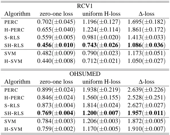
Table 1: Experimental results on two hierarchical text classification tasks under various loss func-tions. We report average test errors along with standard deviations (in parentheses). In bold are the best performance figures among the incremental algorithms (all incremental algorithms were run for one epoch over the training data).

performance of these algorithms was evaluated against three different loss measures (see Table 1). The first two losses are the zero-one loss and the H-loss with cost coefficients set to 1 (denoted by uniform H-loss in Table 1). The third loss is the symmetric difference loss (∆-loss in Table 1).

A few remarks on Table 1 are in order at this point. As expected,H-SVMperforms best, but the

good performance ofSVM(flat support vector machine) is surprising. As for the incremental

algo-rithms, SH-RLS performs better than its flat variantSH-RLS, and far better than both H-PERCand

PERC. In addition, and perhaps surprisingly, after a single epoch of trainingSH-RLSperforms

gen-erally better thanSVMand comes reasonably close to the performance ofH-SVM. Finally, note that

the running times of bothS-RLSandSH-RLSscale quadratically in the number of stored instances, whereas the running time of Perceptrons scales only linearly. Thus, as usual, the performance ben-efit has to be traded-off against computational cost.

To give an idea of how flat and hierarchical algorithms compare in terms of running times, we mention that hierarchical algorithms turned out to be roughly four times faster than the correspond-ing flat algorithms runncorrespond-ing on the same data sets.

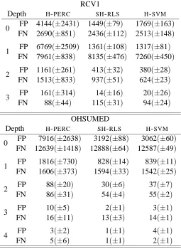
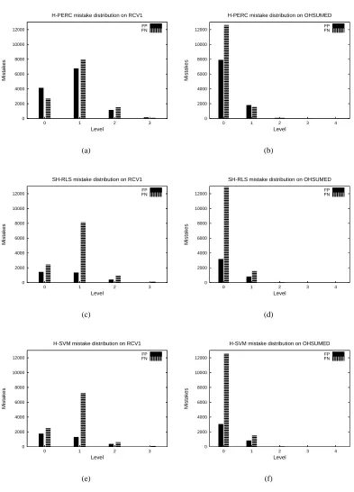
The (uniform) H-loss does not provide any information on the distribution of mistakes across the different hierarchy levels. Therefore, we counted the “H-loss mistakes” made at each level, distinguishing between false positive (FP) and false negative (FN) mistakes. Fix an example(x,v)

and letby be the guessed multilabel. Then node i makes an H-loss mistake on(x,v)if

b

RCV1

Depth H-PERC SH-RLS H-SVM

FP 4144(_±2431) 1449(_±79) 1769(_±163)

0

FN 2690(_±851) 2436(_±112) 2513(_±148)

FP 6769(_±2509) 1361(_±108) 1317(_±81)

1

FN 7961(_±838) 8135(_±476) 7260(_±450)

FP 1161(_±261) 413(_±32) 380(_±28)

2

FN 1513(_±833) 937(_±51) 624(_±23)

FP 161(_±314) 14(_±16) 20(_±26)

3

FN 88(_±44) 115(_±31) 94(_±24)

OHSUMED

Depth H-PERC SH-RLS H-SVM

FP 7916(_±2638) 3192(_±88) 3062(_±60)

0

FN 12639(_±1418) 12888(_±64) 12587(_±49)

FP 1816(_±730) 828(_±14) 839(_±11)

1

FN 1606(_±373) 1594(_±33) 1542(_±25)

FP 88(_±20) 30(_±6) 37(_±7)

2

FN 86(_±31) 54(_±4) 55(_±2)

FP 10(_±5) 2(_±1) 3(_±1)

3

FN 16(_±11) 13(_±3) 14(_±1)

FP 3(_±2) 1(_±1) 4(_±1)

4

FN 5(_±6) 1(_±1) 2(_±1)

Thus, node i makes a false positive mistake if

b

yi=1∧vi=0∧byj=vj=1,j∈ANC(i)

and makes a false negative mistake if

b

yi=0∧vi=1∧ybj=vj=1, j∈ANC(i).

Table 2 shows the H-loss mistake distribution for RCV1 and OHSUMED over hierarchy levels. The average values contained in Table 2 are also plotted in Figure 4. A quick visual comparison reveals the close similarity between the distributions obtained bySH-RLSandH-SVM, whereas the

behavior ofH-PERClooks quite different.

9. Conclusions, Ongoing Research, and Open Problems

We have introducedH-RLS, a new on-line algorithm for hierarchical classification that maintains

and updates regularized least-squares estimators on the nodes of a taxonomy. The linear-threshold classifications, obtained from the estimators, are combined to produce a single hierarchical multil-abel through a simple top-down evaluation model.

Our algorithm is suitable for learning multilabels that include multiple and/or partial paths on the taxonomy. To properly evaluate hierarchical classifiers in this framework we have defined the H-loss, a new hierarchical loss function, with cost coefficients possibly associated to each taxonomy node—see Remark 5.

Our main theoretical result states that, on any sequence of instances, the cumulative H-loss of

H-RLSis never much bigger than the cumulative H-loss of a reference classifier tuned with the

pa-rameters of the stochastic process generating the multilabels for the given sequence of instances. Our theoretical findings are complemented by experiments on the hierarchical classification of tex-tual data, in which we compare the performance of a sparsified variant ofH-RLSto that of standard batch and incremental learners, such as simple hierarchical versions of the Perceptron algorithm and the SVM. The experiments show that one epoch of training of our algorithm is enough to achieve a performance close to that of the hierarchical SVM.

Our investigation leaves a number of open questions. The first open question is the derivation of a hierarchical algorithm especially designed to minimize the H-loss. We are currently exploring efficient ways to approximate the Bayes optimal classifier for the H-loss, given our data model. Since such optimal classifier turns out to be remarkably different from the hierarchical classifiers

produced by H-RLS, a related theoretical question is to prove any reasonable bound on the regret

with respect to the Bayes optimal classifier.

Additional open problems concern the data model. First, it would be useful to modify the label-generating model to introduce dependencies among the children’s labels. This could allow a better fitting of data sets when the rate of multiple paths in multilabels is limited. Second, further investi-gation, both of empirical and theoretical nature, might be devoted to the issue of using regularized logistic regressors at each node.

Acknowledgments

0 2000 4000 6000 8000 10000 12000 3 2 1 0 Mistakes Level

H-PERC mistake distribution on RCV1

FP FN (a) 0 2000 4000 6000 8000 10000 12000 4 3 2 1 0 Mistakes Level

H-PERC mistake distribution on OHSUMED

FP FN (b) 0 2000 4000 6000 8000 10000 12000 3 2 1 0 Mistakes Level

SH-RLS mistake distribution on RCV1

FP FN (c) 0 2000 4000 6000 8000 10000 12000 4 3 2 1 0 Mistakes Level

SH-RLS mistake distribution on OHSUMED

FP FN (d) 0 2000 4000 6000 8000 10000 12000 3 2 1 0 Mistakes Level

H-SVM mistake distribution on RCV1

FP FN (e) 0 2000 4000 6000 8000 10000 12000 4 3 2 1 0 Mistakes Level

H-SVM mistake distribution on OHSUMED

FP FN

(f)

This work was supported in part by the IST Programme of the European Community under the PAS-CAL Network of Excellence IST-2002-506778. This publication only reflects the authors’ views.

Appendix A

This appendix contains the proofs of Lemmas 7, 8, and 9 mentioned in the main text. Throughout this appendix A denotes the positive definite matrix I+Si,QS>i,Q, while r denotes the quadratic form

x>_t (A+xtx>t )−1xt.

Proof of Lemma 7 We have

Bi,t = u>i (I+xtxt>)(A+xtx>t )−1xt = u>_i (A+xtxt>)−1xt+∆i,tr

≤

q

x>_t (A+xtx>t )−2xt+|∆i,t|r

≤ √r+_|∆i,t|r

where the first inequality follows from u>_i z_≤max_kuik=1u>_i z=_kz_k, with z= (A+xtxt>)−1xt, and the

second inequality follows from x>(A+xx>)−2_{x≤x>(A+xx>)−}1_{x, holding for any x and for any} positive definite matrix A whose eigenvalues are not smaller than 1 (notice that this condition makes

(A+xx>)−1_−(A+xx>₎−2_{a positive semidefinite matrix).}

Proof of Lemma 8

Setting for brevity H=S>_i,QA−1xt and a=x>t A−1xt we can write

kZi,tk2 = x>t

A+xtx>t

−1

Si,QS>i,Q

A+xtx>t

−1 xt

= x>_t

A−1₋A −1_x

tx>t A−1

1+x>_t A−1_x

t

Si,QS>i,Q

A−1₋A −1_x

tx>t A−1

1+x>_t A−1_x

t

xt

(by the Sherman-Morrison formula—e.g., Horn and Johnson, 1985, chap. 0)

= H>H− a

1+aH

>_H− a

1+aH

>_H+ a2

(1+a)2H>H

= H>H

(1+a)2

= x

>

t A−1Si,QS>_i,QA−1xt (1+a)2

= x

>

t A−1/2A−1/2Si,QS>i,QA−1/2A−1/2xt (1+a)2

≤

A−1/2xt

A−1/2Si,QS>i,QA−1/2

x_t>A−1/2

(1+a)2

= a

(1+a)2

A−1/2Si,QS>i,QA−1/2

where

A−1/2Si,QS_i>_,QA−1/2

is the spectral norm of matrix A−1/2Si,QS>_i,QA−1/2.

We continue by bounding the two factors in (16). Observe that

a

(1+a)2 ≤ a

1+a=r

where the equality derives again from the Sherman-Morrison formula. As far as the second factor is concerned, we just note that the two matrices A−1/2 and Si,QS>i,Q have the same eigenvectors.

Furthermore, ifλjis an eigenvalue of Si,QS>i,Q, then 1/

p

1+λjis an eigenvalue of A−1/2. Therefore

A−1/2Si,QSi>,QA−1/2

=max

j

1 p

1+λj×

λj×

1 p

1+λj ≤

1.

Substituting into (16) yields_kZi,tk2≤r,as desired.

Proof of Lemma 9

From a simple Kuhn-Tucker analysis3it follows that if at is larger than 0 at the maximum, then at

takes some constant valueβ>0 (independent of t). Hence the maximizing vector(a1,a2, . . . ,an)

has components which can take only two possible values: at=0 or at =β. Let us denote by N+the

number of t : at =β. At the maximum we can write

M= n

∑

t=1

at =

∑

at+

∑

at =βN+

i.e.,β=M/N+. Hence, at the maximum

n

∑

t=1

e−α/at ₌

∑

e−α/at₊

∑

e−α/at

=

∑

t : at=β

e−α/β

= N+e−α/β

= N+e−αN+/M.

Since N+is not determined by this argument, we can write

max ( _n

∑

t=1

e−α/at _{: a1≥0, . . . ,a} n≥0,

n

∑

t=1 at =M

)

≤max

x≥0 x e

−αx/M₌ M

eα

thereby concluding the proof.