Maximum Entropy Density Estimation with Generalized
Regularization and an Application to Species Distribution Modeling
Miroslav Dud´ık [email protected]
Princeton University
Department of Computer Science 35 Olden Street
Princeton, NJ 08540
Steven J. Phillips [email protected]
AT&T Labs−Research 180 Park Avenue Florham Park, NJ 07932
Robert E. Schapire [email protected]
Princeton University
Department of Computer Science 35 Olden Street
Princeton, NJ 08540
Editor: John Lafferty
Abstract
We present a unified and complete account of maximum entropy density estimation subject to constraints represented by convex potential functions or, alternatively, by convex regularization. We provide fully general performance guarantees and an algorithm with a complete convergence proof. As special cases, we easily derive performance guarantees for many known regularization types, including`1,`2,`2
2, and`1+`22style regularization. We propose an algorithm solving a large and general subclass of generalized maximum entropy problems, including all discussed in the paper, and prove its convergence. Our approach generalizes and unifies techniques based on information geometry and Bregman divergences as well as those based more directly on compactness. Our work is motivated by a novel application of maximum entropy to species distribution modeling, an important problem in conservation biology and ecology. In a set of experiments on real-world data, we demonstrate the utility of maximum entropy in this setting. We explore effects of different feature types, sample sizes, and regularization levels on the performance of maxent, and discuss interpretability of the resulting models.
Keywords: maximum entropy, density estimation, regularization, iterative scaling, species distri-bution modeling
1. Introduction
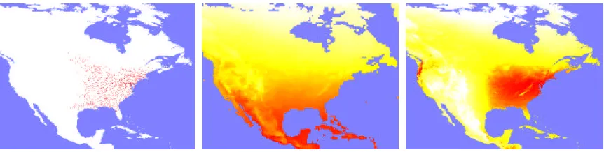
Figure 1: Left to right: Yellow-throated Vireo training localities from the first random partition, an example environmental variable (annual average temperature, higher values in red), max-ent prediction using linear, quadratic and product features. Prediction strength is shown as white (weakest) to red (strongest); reds could be interpreted as suitable conditions for the species.
the given constraints. The constraints are often represented using a set of features (real-valued functions) on the space, with the expectation of every feature required to match its empirical average. By convex duality, this turns out to be the unique Gibbs distribution maximizing the likelihood of the samples, or, equivalently, minimizing the empirical log loss. (Maxent and its dual are described more rigorously in Section 2.)
The work in this paper was motivated by a new application of maxent to the problem of modeling the distribution of a plant or animal species, a critical problem in conservation biology. Input data for species distribution modeling consists of occurrence locations of a particular species in a region and of environmental variables for that region. Environmental variables may include topographical layers, such as elevation and aspect, meteorological layers, such as annual precipitation and average temperature, as well as categorical layers, such as vegetation and soil type. Occurrence locations are commonly derived from specimen collections in natural history museums and herbaria. In the context of maxent, occurrences correspond to samples, the map divided into a finite number of cells is the sample space, and environmental variables or functions derived from them are features (see Figure 1 for an example). The number of occurrences for individual species is frequently quite small by machine learning standards, for example, a hundred or less.
and constraint relaxation (Khudanpur, 1995; Kazama and Tsujii, 2003; Jedynak and Khudanpur, 2005). Thus, there are many ways of modifying maxent to control overfitting calling for a general treatment.
In this work, we study a generalized form of maxent. Although mentioned by other authors as fuzzy maxent (Lau, 1994; Chen and Rosenfeld, 2000; Lebanon and Lafferty, 2001), we give the first complete theoretical treatment of this very general framework, including fully general and unified performance guarantees, algorithms, and convergence proofs. Independently, Altun and Smola (2006) derive a different theoretical treatment (see discussion below).
As special cases, our results allow us to easily derive performance guarantees for many known regularized formulations, including `1, `2, `22, and `1+`22 regularizations. More specifically, we
derive guarantees on the performance of maxent solutions compared to the “best” Gibbs distribution
q? defined by a weight vectorλ?. Our guarantees are derived by bounding deviations of empirical feature averages from their expectations, a setting in which we can take advantage of a wide array of uniform convergence results. For example, for a finite set of features bounded in[0,1], we can use Hoeffding’s inequality and the union bound to show that the true log loss of the`1-regularized
maxent solution will be with high probability worse by no more than an additive O(kλ?k1p(ln n)/m) compared with the log loss of the Gibbs distribution q?, where n is the number of features and m is the number of samples. For an infinite set of binary features with VC-dimension d, the difference between the`1-regularized maxent solution and q?is at most O(kλ?k1
p
d ln(m2/d)/m). Note that
these bounds drop quickly with an increasing number of samples and depend only moderately on the number or complexity of the features, even admitting an extremely large number of features from a class of bounded VC-dimension. For maxent with`2 and`22-style regularization, it is possible to
obtain bounds which are independent of the number of features, provided that the feature vector can be bounded in the`2norm.
In the second part, we propose algorithms solving a large and general subclass of generalized maxent problems. We show convergence of our algorithms using a technique that unifies previous approaches and extends them to a more general setting. Specifically, our unified approach general-izes techniques based on information geometry and Bregman divergences (Della Pietra et al., 1997, 2001; Collins et al., 2002) as well as those based more directly on compactness. The main novel ingredient is a modified definition of an auxiliary function, a customary measure of progress, which we view as a surrogate for the difference between the primal and dual objective rather than a bound on the change in the dual objective.
Standard maxent algorithms such as iterative scaling (Darroch and Ratcliff, 1972; Della Pietra et al., 1997), gradient descent, Newton and quasi-Newton methods (Cesa-Bianchi et al., 1994; Mal-ouf, 2002; Salakhutdinov et al., 2003), and their regularized versions (Lau, 1994; Williams, 1995; Chen and Rosenfeld, 2000; Kazama and Tsujii, 2003; Goodman, 2004; Krishnapuram et al., 2005) perform a sequence of feature weight updates until convergence. In each step, they update all fea-ture weights. This is impractical when the number of feafea-tures is very large. Instead, we propose a sequential update algorithm that updates only one feature weight in each iteration, along the lines of algorithms studied by Collins, Schapire, and Singer (2002), and Lebanon and Lafferty (2001). This leads to a boosting-like approach permitting the selection of the best feature from a very large class. For instance, for`1-regularized maxent, the best threshold feature associated with a single variable
For cases when the number of features is relatively small, yet we want to use benefits of regu-larization to prevent overfitting on small sample sets, it might be more efficient to solve generalized maxent by parallel updates. In Section 7, we give a parallel-update version of our algorithm with a proof of convergence.
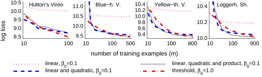
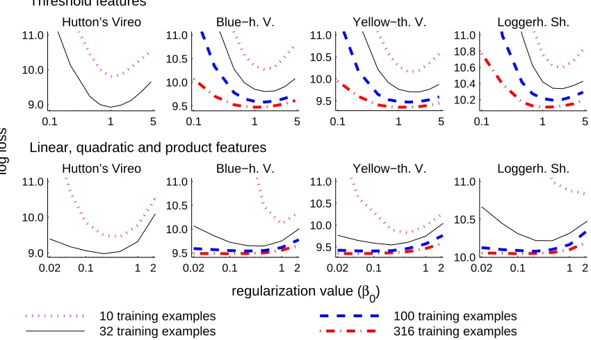
In the last section, we return to species distribution modeling, and use it as a setting to test our ideas. In particular, we apply`1-regularized maxent to estimate distributions of bird species in North
America. We present learning curves for several different feature classes derived for four species with a varying number of occurrence records. We also explore effects of regularization on the test log loss and interpretability of the resulting models. A more comprehensive set of experiments is evaluated by Phillips, Dud´ık, and Schapire (2004). The biological application is explored in more detail by Phillips, Anderson, and Schapire (2006).
1.1 Previous Work
There have been many studies of maxent and logistic regression, which is a conditional version of maxent, with`1-style regularization (Khudanpur, 1995; Williams, 1995; Kazama and Tsujii, 2003;
Ng, 2004; Goodman, 2004; Krishnapuram et al., 2005),`2
2-style regularization (Lau, 1994; Chen
and Rosenfeld, 2000; Lebanon and Lafferty, 2001; Zhang, 2005) as well as some other types of regularization such as`1+`22-style (Kazama and Tsujii, 2003), `2-style regularization (Newman,
1977) and a smoothed version of`1-style regularization (Dekel et al., 2003). In a recent work, Altun
and Smola (2006) derive duality and performance guarantees for settings in which the entropy is replaced by an arbitrary Bregman or Csisz´ar divergence and regularization takes the form of a norm raised to a power greater than one. With the exception of Altun and Smola’s work and Zhang’s work, the previous studies do not give performance guarantees applicable to our case, although Kr-ishnapuram et al. (2005) and Ng (2004) prove guarantees for`1-regularized logistic regression. Ng
also shows that `1-regularized logistic regression may be superior to the`22-regularized version in
a scenario when the number of features is large and only a small number of them is relevant. Our results indicate a similar behavior for unconditional maxent.
In the context of linear models, `2
2, `1, and `1+`22 regularization have been used under the
names ridge regression (Hoerl and Kennard, 1970), lasso regression (Tibshirani, 1996), and elastic
nets (Zou and Hastie, 2005). Lasso regression, in particular, has provoked a lot of interest in recent
statistical theory and practice. The frequently mentioned benefit of the lasso is its bias toward sparse solutions. The same bias is present also in`1-regularized maxent, but we do not analyze this bias
in detail. Our interest is in deriving performance guarantees. Similar guarantees were derived by Donoho and Johnstone (1994) for linear models with the lasso penalty. The relationship between the lasso approximation and the sparsest approximation is explored, for example, by Donoho and Elad (2003).
Quite a number of approaches have been suggested for species distribution modeling, including neural nets, nearest neighbors, genetic algorithms, generalized linear models, generalized additive models, bioclimatic envelopes, boosted regression trees, and more; see Elith (2002) and Elith et al. (2006) for a comprehensive comparison. The latter work evaluates `1-regularized maxent as one
Among these, however, maxent is the only method designed for presence-only data. It comes with a statistical interpretation that allows principled extensions, for example, to cases where the sampling process is biased (Dud´ık et al., 2005).
2. Preliminaries
Our goal is to estimate an unknown densityπover a sample space
X
which, for the purposes of this paper, we assume to be finite.1 As empirical information, we are typically given a set of samples x1, . . . ,xmdrawn independently at random according toπ. The corresponding empirical distributionis denoted by ˜π:
˜
π(x) =|{1≤i≤m : xi=x}|
m .
We also are given a set of features f1, . . . ,fn where fj :
X
→R. The vector of all n features isdenoted by f and the image of
X
under f, the feature space, is denoted by f(X). For a distributionπ and function f , we writeπ[f]to denote the expected value of f under distributionπ:π[f] =∑x∈Xπ(x)f(x) .
In general, ˜πmay be quite distant, under any reasonable measure, fromπ. On the other hand, for a given function f , we do expect ˜π[f], the empirical average of f , to be rather close to its true expectationπ[f]. It is quite natural, therefore, to seek an approximation p under which fj’s
expectation is equal to ˜π[fj]for every fj. There will typically be many distributions satisfying these
constraints. The maximum entropy principle suggests that, from among all distributions satisfying these constraints, we choose the one of maximum entropy, that is, the one that is closest to uniform. Here, as usual, the entropy of a distribution p on
X
is defined to be H(p) =−∑x∈Xp(x)ln p(x).However, the default estimate ofπ, that is, the distribution we would choose if we had no sample data, may be in some cases non-uniform. In a more general setup, we therefore seek a distribution that minimizes entropy relative to the default estimate q0. The relative entropy, or Kullback-Leibler
divergence, is an information theoretic measure defined as
D(pkq) =p[ln(p/q)] .
Minimizing entropy relative to q0corresponds to choosing a distribution that is closest to q0. When q0is uniform then minimizing entropy relative to q0is equivalent to maximizing entropy.
Instead of minimizing entropy relative to q0, we can consider all Gibbs distributions of the form qλ(x) =
q0(x)eλ·f(x) Zλ
where Zλ=∑x∈Xq0(x)eλ·f(x)is a normalizing constant, andλ∈Rn. It can be proved (Della Pietra
et al., 1997) that the maxent distribution is the same as the maximum likelihood distribution from the closure of the set of Gibbs distributions, that is, the distribution q that achieves the supremum of∏mi=1qλ(xi)over all values ofλ, or equivalently, the infimum of the empirical log loss (negative
normalized log likelihood)
Lπ˜(λ) =−
1
m
m
∑
i=1
ln qλ(xi) .
1. In this paper, we are concerned with densities relative to the counting measure onX. These correspond to probability
The convex programs corresponding to the two optimization problems are
min
p∈∆D(pkq0)subject to p[f] =π˜[f] , (1)
inf
λ∈RnLπ˜(
λ) (2)
where∆is the simplex of probability distributions over
X
. In general, we useLr(λ) =−r[ln qλ]
to denote the log loss of qλrelative to the distribution r. It differs from relative entropy D(rkqλ)
only by the constant H(r). We will use the two interchangeably as objective functions.
3. Convex Analysis Background
Throughout this paper we make use of convex analysis. The necessary background is provided in this section. For a more detailed exposition see for example Rockafellar (1970), or Boyd and Vandenberghe (2004).
Consider a functionψ:Rn→(−∞,∞]. The effective domain ofψis the set domψ={u∈Rn:
ψ(u)<∞}. A point u whereψ(u)<∞is called feasible. The epigraph ofψ is the set of points
above its graph{(u,t)∈Rn×R: t ≥ψ(u)}. We say thatψis convex if its epigraph is a convex
set. A convex function is called proper if it is not uniformly equal to∞. It is called closed if its
epigraph is closed. For a proper convex function, closedness is equivalent to lower semi-continuity (ψis lower semi-continuous if lim infu0→uψ(u0)≥ψ(u)for all u).
Ifψis a closed proper convex function then its conjugateψ∗:Rn→(−∞,∞]is defined by
ψ∗(λ) = sup
u∈Rn
[λ·u−ψ(u)] .
The conjugate provides an alternative description ofψ in terms of tangents ofψ’s epigraph. The definition of the conjugate immediately yields Fenchel’s inequality
∀λ,u : λ·u≤ψ∗(λ) +ψ(u) .
In fact,ψ∗(λ)is defined to give the tightest bound of the form above. It turns out thatψ∗ is also a closed proper convex function andψ∗∗=ψ(for a proof see Rockafellar, 1970, Corollary 12.2.1).
In this work we use several examples of closed proper convex functions. The first of them is relative entropy, viewed as a function of its first argument and extended toRX as follows:
ψ(p) =
(
D(pkq0) if p∈∆
∞ otherwise
where q0∈∆is assumed fixed. The conjugate of relative entropy is the log partition function
ψ∗(r) =ln∑x∈Xq0(x)er(x)
The second example is the unnormalized relative entropy
e
D(pkq0) =∑x∈X
p(x)ln
p(x)
q0(x)
−p(x) +q0(x)
.
Fixing q0∈[0,∞)X, it can be extended to a closed proper convex function of its first argument:
ψ(p) =
( e
D(pkq0) if p(x)≥0 for all x∈
X
∞ otherwise.
The conjugate of unnormalized relative entropy is a scaled exponential shifted to the origin:
ψ∗(r) =∑x∈Xq0(x)(er(x)−1) .
Both relative entropy and unnormalized relative entropy are examples of Bregman divergences (Bregman, 1967) which generalize some common distance measures including the squared Eu-clidean distance. We use two properties satisfied by any Bregman divergence B(· k ·):
(B1) B(akb)≥0 ,
(B2) if B(at kbt)→0 and bt →b?then at→b?.
It is not too difficult to check these properties explicitly both for relative entropy and unnormalized relative entropy.
Another example of a closed proper convex function is an indicator function of a closed convex set C⊆Rn, denoted by IC, which equals 0 when its argument lies in C and infinity otherwise. We
will also use I(u∈C)to denote IC(u). The conjugate of an indicator function is a support function.
For C={u0}, we obtain I∗{u
0}(
λ) =λ·u0. For a box R={u :|uj| ≤βj for all j}, we obtain an `1-style conjugate I∗R(λ) =∑jβj|λj|. For a Euclidean ball B={u :kuk2≤β}, we obtain an`2-style
conjugate, I∗B(λ) =βkλk2.
The final example is a square of the Euclidean normψ(u) =kuk22/(2α), whose conjugate is also a square of the Euclidean normψ∗(λ) =αkλk2
2/2.
The following identities can be proved from the definition of the conjugate function:
ifϕ(u) =aψ(bu+c) thenϕ∗(λ) =aψ∗(λ/(ab))−λ·c/b , (3)
ifϕ(u) =∑jϕj(uj) thenϕ∗(λ) =∑jϕ∗j(λj) (4)
where a>0,b6=0 and c∈Rnare constants, and uj,λjrefer to the components of u,λ.
We conclude with a version of Fenchel’s Duality Theorem which relates a convex minimization problem to a concave maximization problem using conjugates. The following result is essentially Corollary 31.2.1 of Rockafellar (1970) under a stronger set of assumptions.
Theorem 1 (Fenchel’s Duality). Letψ:Rn→(−∞,∞]andϕ:Rm→(−∞,∞]be closed proper
convex functions and A a real-valued m×n matrix. Assume that domψ∗=Rnor domϕ=Rm. Then
inf
u
ψ(u) +ϕ(Au)=sup
λ
−ψ∗(A>λ)−ϕ∗(−λ) .
4. Generalized Maximum Entropy
In this paper we study a generalized maxent problem
P
: minp∈∆
D(pkq0) +U(p[f])
where U :Rn→(−∞,∞]is an arbitrary closed proper convex function. It is viewed as a potential
for the maxent problem. We further assume that q0is positive on
X
, that is, D(pkq0)is finite forall p∈∆(otherwise we could restrict
X
to the support of q0), and there exists a distribution whosevector of feature expectations is a feasible point of U (this is typically satisfied by the empirical distribution). These two conditions imply that the problem
P
is feasible.The definition of generalized maxent captures many cases of interest including basic maxent,`1
-regularized maxent and`2
2-regularized maxent. Basic maxent is obtained by using a point indicator
potential U(0)(u) =I(u=π˜[f]). The `
1-regularized version of maxent, as shown by Kazama and
Tsujii (2003), corresponds to the relaxation of equality constraints to box constraints
|π˜[fj]−p[fj]| ≤βj .
This choice can be motivated by an observation that we do not expect ˜π[fj] to be equal to π[fj]
but only close to it. Box constraints are represented by the potential U(1)(u) =I(|π˜[f
j]−uj| ≤
βj for all j). Finally, as pointed out by Chen and Rosenfeld (2000) and Lebanon and Lafferty
(2001), `2
2-regularized maxent is obtained using the potential U(
2)(u) =kπ˜[f]−uk2
2/(2α) which
incurs an`2
2-style penalty for deviating from empirical averages.
The primal objective of generalized maxent will be referred to as P:
P(p) =D(pkq0) +U(p[f]) .
Note that P attains its minimum over∆, because∆is compact and P is lower semi-continuous. The minimizer of P is unique by strict convexity of D(pkq0).
To derive the dual of
P
, define the matrix Fjx= fj(x)and use Fenchel’s duality:min
p∈∆[D(pkq0) +U(p[f])] =minp∈∆[D(pkq0) +U(Fp)]
= sup
λ∈Rn
h
−ln
∑x∈Xq0(x)exp
(F>λ)x −U∗(−λ)i (5)
= sup
λ∈Rn
[−ln Zλ−U∗(−λ)] . (6)
In Equation (5), we apply Theorem 1. We use (F>λ)x to denote the entry of F>λ indexed by x. In Equation (6), we note that (F>λ)x=λ·f(x) and thus the expression inside the logarithm is the normalization constant of qλ. The dual objective will be referred to as Q:
Q(λ) =−ln Zλ−U∗(−λ) .
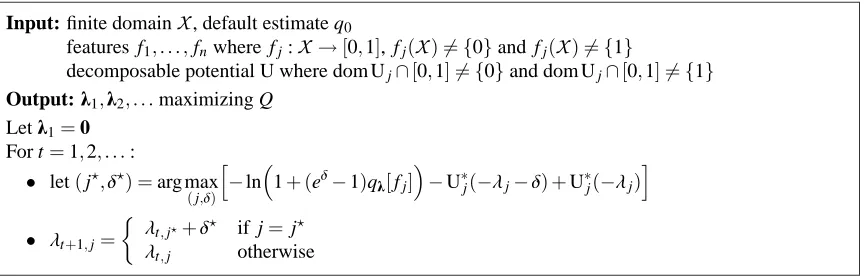
potential (absolute and relative) conjugate potential generalized maxent:
U(u) U(u) U∗(λ)
Ur(u) U(r[f]−u) U∗(−λ) +λ·r[f]
Uπ(u)˜ U(π˜[f]−u) U∗(−λ) +λ·π˜[f] basic constraints:
U(0)(u) I(u=π˜[f]) λ·π˜[f] Ur(0)(u) I(u=r[f]−π˜[f]) λ·(r[f]−π˜[f])
U(π˜0)(u) I(u=0) 0
box constraints:
U(1)(u) I(|π˜[f
j]−uj| ≤βjfor all j) λ·π˜[f] +∑jβj|λj|
U(r1)(u) I(|uj−(r[fj]−π˜[fj])| ≤βjfor all j) λ·(r[f]−π˜[f]) +∑jβj|λj|
U(π˜1)(u) I(|uj| ≤βjfor all j) ∑jβj|λj|
`2
2penalty:
U(2)(u) kπ˜[f]−uk2
2/(2α) λ·π˜[f] +αkλk22/2 U(r2)(u) ku−(r[f]−π˜[f])k22/(2α) λ·(r[f]−π˜[f]) +αkλk22/2 U(π˜2)(u) kuk22/(2α) αkλk2
2/2
Table 1: Absolute and relative potentials, and their conjugates for various versions of maxent.
the example of U(0). In the latter case, it would be more correct, but perhaps overly pedantic and somewhat clumsy, to make the dependence of the potential on ˜πexplicit and use the notation U(0),π˜.
The second difference, which seems more significant, is the difference between the duals. The objective of the basic dual (2) equals the log loss relative to the empirical distribution ˜π, but the log loss does not appear in the generalized dual. However, we will see that the generalized dual can be expressed in terms of the log loss. In fact, it can be expressed in terms of the log loss relative to an arbitrary distribution, including the empirical distribution ˜πas well as the unknown distributionπ.
We next describe shifting, the transformation of an “absolute” potential to a “relative” potential. Shifting is a technical tool which will simplify some of the proofs in Sections 5 and 6, and will also be used to rewrite the generalized dual in terms of the log loss.
4.1 Shifting
For an arbitrary distribution r and a potential U, let Urdenote the function
Ur(u) =U(r[f]−u) .
This function will be referred to as the potential relative to r or simply the relative potential. The original potential U will be in contrast referred to as the absolute potential. In Table 1, we list potentials discussed so far, alongside their versions relative to an arbitrary distribution r, and relative to ˜πin particular.
From the definition of a relative potential, we see that the absolute potential can be expressed as U(u) =Ur(r[f]−u). Thus, it is possible to implicitly define a potential U by defining a relative
potential Urfor a particular distribution r. The potentials U(0), U(1), U(2)of basic maxent, maxent with
box constraints, and maxent with`2
2 penalty could thus have been specified by defining U (0) ˜ π (u) = I(u=0), U(π˜1)(u) =I(|uj| ≤βjfor all j)and U(
2) ˜
The conjugate of a relative potential, the conjugate relative potential, is obtained, according to Equation (3), by adding a linear function to the conjugate of U:
U∗r(λ) =U∗(−λ) +λ·r[f] . (7)
Table 1 lists U(0)∗, U(1)∗, U(2)∗, and the conjugates of the corresponding relative potentials.
4.2 The Generalized Dual as the Minimization of a Regularized Log Loss
We will now show how the dual objective Q(λ)can be expressed in terms of the log loss relative to an arbitrary distribution r. This will highlight how the dual of the generalized maxent extends the dual of the basic maxent. Using Equation (7), we rewrite Q(λ)as follows:
Q(λ) =−ln Zλ−U∗(−λ) =−ln Zλ−U∗
r(λ) +λ·r[f]
=−r[ln q0] +r[ln q0+λ·f−ln Zλ]−U∗r(λ)
=Lr(0)−Lr(λ)−U∗r(λ) . (8)
Since the first term in Equation (8) is a constant independent of λ, the maximization of Q(λ) is equivalent to the minimization of Lr(λ) +U∗r(λ). Setting r=π˜ we obtain a dual analogous to the
basic dual (2):
Q
π˜: infλ∈Rn
h
Lπ˜(λ) +U∗π˜(λ) i
.
From Equation (8), it follows that the λ minimizing Lr(λ) +U∗
r(λ) does not depend on a
partic-ular choice of r. As a result, the minimizer of
Q
π˜ is also the minimizer of Lπ(λ) +U∗π(λ). This observation will be used in Section 5 to prove performance guarantees.The objective of
Q
π˜ has two terms. The first of them is the empirical log loss. The secondone is the regularization term penalizing “complex” solutions. The regularization term need not be non-negative and it does not necessarily increase with any norm ofλ. On the other hand, it is a proper closed convex function and if ˜πis feasible then by Fenchel’s inequality the regularization is bounded from below by−Uπ˜(0). From a Bayesian perspective, U∗π˜ corresponds to negative log of
the prior, and minimizing Lπ˜(λ) +U∗π˜(λ)is equivalent to maximizing the posterior.
In the case of basic maxent, we obtain U(π˜0)∗(λ) =0 and recover the basic dual. For the box potential, we obtain U(π˜1)∗(λ) =∑
jβj|λj|, which corresponds to an `1-style regularization and a
Laplace prior. For the`2
2potential, we obtain U (2)∗ ˜
π (λ) =αkλk22/2, which corresponds to an`22-style
regularization and a Gaussian prior.
In all the cases discussed in this paper, it is natural to consider the dual objective relative to ˜π as we have seen in the previous examples. In other cases, the empirical distribution ˜πneed not be available, and there may be no natural distribution relative to which a potential could be specified, yet it is possible to define a meaningful absolute potential (Dud´ık et al., 2005; Dud´ık and Schapire, 2006). To capture the more general case, we formulate the generalized maxent using the absolute potential.
4.3 Maxent Duality
(possibly in a limit). This parallels the result of Della Pietra, Della Pietra, and Lafferty (1997) for the basic maxent and gives additional motivation for the view of the dual objective as the regularized log loss.
Theorem 2 (Maxent Duality). Let q0,U,P,Q be as above. Then
min
p∈∆P(p) =λsup∈Rn
Q(λ) . (9)
Moreover, for a sequenceλ1,λ2, . . .such that lim
t→∞
Q(λt) = sup
λ∈Rn Q(λ)
the sequence of qt=qλt has a limit and
Plim
t→∞
qt
=min
p∈∆P(p) . (10)
Proof. Equation (9) is a consequence of Fenchel’s duality as was shown earlier. It remains to prove
Equation (10). We will use an alternative expression for the dual objective. Let r be an arbitrary distribution. Adding and subtracting H(r)from Equation (8) yields
Q(λ) =−D(rkqλ) +D(rkq0)−U∗r(λ) . (11) Let ˆp be the minimizer of P andλ1,λ2, . . .maximize Q in the limit. Then
D(pˆkq0) +Upˆ(0) =P(pˆ) = sup
λ∈Rn
Q(λ) = lim
t→∞
Q(λt)
= lim
t→∞
−D(pˆkqt) +D(pˆkq0)−U∗pˆ(λt)
.
Denoting terms with the limit 0 by o(1)and rearranging yields
Upˆ(0) +U∗pˆ(λt) =−D(pˆkqt) +o(1) .
The left-hand side is non-negative by Fenchel’s inequality, so D(pˆkqt)→0 by the non-negativity
of relative entropy. Therefore, by property(B2), every convergent subsequence of q1,q2, . . .has the
limit ˆp. Since the qt’s come from the compact set∆, we obtain qt→ p.ˆ
Thus, in order to solve the primal, it suffices to find a sequence ofλ’s maximizing the dual. This will be the goal of algorithms in Sections 6 and 7.
5. Bounding the Loss on the Target Distribution
In this section, we derive bounds on the performance of generalized maxent relative to the true distributionπ. That is, we are able to bound Lπ(λˆ)in terms of Lπ(λ?)when qˆλmaximizes the dual
objective Q and qλ? is either an arbitrary Gibbs distribution, or in some cases, a Gibbs distribution
with a bounded norm ofλ?. In particular, bounds hold for the Gibbs distribution minimizing the true loss (in some cases, among Gibbs distributions with a bounded norm of λ?). Note that D(πkqλ) differs from Lπ(λ)only by the constant term H(π), so identical bounds also hold for D(πkqλˆ)in
Our results are stated for the case when the supremum of Q is attained at ˆλ∈Rn, but they easily
extend to the case when the supremum is only attained in a limit. The crux of our method is the lemma below. Even though its proof is remarkably simple, it is sufficiently general to cover all the cases of interest.
Lemma 3. Let ˆλmaximize Q. Then for an arbitrary Gibbs distribution qλ?
Lπ(ˆλ)≤Lπ(λ?) +2U(π[f]) +U∗(λ?) +U∗(−λ?) , (12) Lπ(ˆλ)≤Lπ(λ?) +2Uπ˜(π˜[f]−π[f]) +U∗π˜(λ?) +U∗π˜(−λ?) , (13)
Lπ(ˆλ)≤Lπ(λ?) + (λ?−ˆλ)·(π[f]−π˜[f]) +U∗π˜(λ?)−U∗π˜(λˆ) . (14) Proof. Optimality of ˆλwith respect to Lπ(λ) +U∗
π(λ) =−Q(λ) +const. yields Lπ(ˆλ)≤Lπ(λ?) +U∗π(λ?)−U∗π(λˆ)
≤Lπ(λ?) + (λ?−ˆλ)·π[f] +U∗(−λ?)−U∗(−λˆ) . (15) In Equation (15), we express U∗πin terms of U∗using Equation (7). Now Equation (12) is obtained by applying Fenchel’s inequality to the second term of Equation (15):
(λ?−ˆλ)·π[f]≤U∗(λ?) +U(π[f]) +U∗(−λˆ) +U(π[f]) .
Equations (13) and (14) follow from Equations (12) and (15) by shifting potentials and their conju-gates to ˜π.
Remark. Notice thatπand ˜πin the statement and the proof of the lemma can be replaced by arbitrary distributions p1and p2.
A special case which we discuss in more detail is when U is an indicator of a closed convex set C, such as U(0)and U(1)of the previous section. In that case, the right hand side of Lemma 3.12 will be infinite unlessπ[f]lies in C. In order to apply Lemma 3.12, we ensure thatπ[f]∈C with high
probability. Therefore, we choose C as a confidence region forπ[f]. Ifπ[f]∈C then for any Gibbs
distribution qλ?
Lπ(ˆλ)≤Lπ(λ?) +IC∗(λ?) +IC∗(−λ?) . (16)
For a fixedλ?and a non-empty C, I∗
C(λ?) +I∗C(−λ?)is always non-negative and proportional to the
size of C’s projection onto a line in the directionλ?. Thus, smaller confidence regions yield better performance guarantees.
A common method of obtaining confidence regions is to bound the difference between empirical averages and true expectations. There exists a huge array of techniques to achieve this. Before moving to specific examples, we state a general result which follows directly from Lemma 3.13 analogously to Equation (16).
Theorem 4. Assume that ˜π[f]−π[f]∈C0 where C0 is a closed convex set symmetric around the origin. Let ˆλminimize Lπ˜(λ) +I∗
C0(λ). Then for an arbitrary Gibbs distribution qλ?
Lπ(λˆ)≤Lπ(λ?) +2IC∗0(λ ?) .
Proof. Setting U˜π(u) =IC0(u)and assuming ˜π[f]−π[f]∈C0, we obtain by Lemma 3.13
Lπ(λˆ)≤Lπ(λ?) +IC∗0(λ?) +IC∗0(−λ?) .
The result now follows by the symmetry of C0, which implies the symmetry of IC0, which in turn
implies the symmetry of IC∗
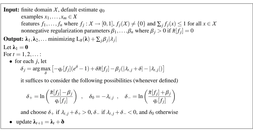
5.1 Maxent with`1Regularization
We now apply the foregoing general results to some specific cases of interest. To begin, we consider the box indicator U(1)of Section 4. In this case it suffices to bound
|π˜[fj]−π[fj]|and use Theorem 4
to obtain a bound on the true loss Lπ(λˆ). For instance, when the features are bounded, we can prove the following:
Corollary 5. Assume that features f1, . . . ,fn are bounded in [0,1]. Let δ>0 and let ˆλ minimize
Lπ˜(λ) +βkλk1 with β= p
ln(2n/δ)/(2m). Then with probability at least 1−δ, for every Gibbs distribution qλ?,
Lπ(ˆλ)≤Lπ(λ?) +k λ?k1
√
m p
2 ln(2n/δ) .
Proof. By Hoeffding’s inequality, for a fixed j, the probability that|π˜[fj]−π[fj]|exceeds β is at
most 2e−2β2m=δ/n. By the union bound, the probability of this happening for any j is at mostδ. The claim now follows immediately from Theorem 4.
Similarly, when the fj’s are selected from a possibly larger class of binary features with
VC-dimension d, we can prove the following corollary. This will be the case, for instance, when using threshold features on k variables, a class with VC-dimension O(ln k).
Corollary 6. Assume that features are binary with VC-dimension d. Letδ>0 and let ˆλminimize Lπ˜(λ) +βkλk1with
β=
r
d ln(em2/d) +ln(1/δ) +ln(4e8)
2m .
Then with probability at least 1−δ, for every Gibbs distribution qλ?,
Lπ(λˆ)≤Lπ(λ?) +k λ?k1
√m
q
2[d ln(em2/d) +ln(1/δ) +ln(4e8)] .
Proof. Here, a uniform-convergence result of Devroye (1982), combined with Sauer’s Lemma, can
be used to argue that|π˜[fj]−π[fj]| ≤βfor all fj simultaneously with probability at least 1−δ.
The final result for `1-regularized maxent is motivated by the Central Limit Theorem
approx-imation |π˜[fj]−π[fj]|=O(σ[fj]/√m), where σ[fj]is the standard deviation of fj underπ. We
boundσ[fj]from above using McDiarmid’s inequality for the empirical estimate of variance
˜ σ2[fj] =
m ˜π[f2
j]−π˜[fj]2
m−1 ,
and then obtain non-asymptotic bounds on|π˜[fj]−π[fj]|by Bernstein’s inequality (for a complete
proof see Appendix A).
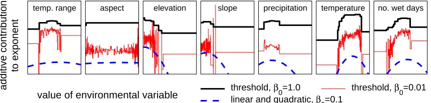
We believe that this type of result may in practice be more useful than Corollaries 5 and 6, because it allows differentiation between features depending on empirical error estimates computed from the sample data. Motivated by Corollary 7 below, in Section 8 we describe experiments that useβj =β0σ˜[fj]/√m, where β0 is a single tuning constant. This approach is equivalent to using
features scaled to the unit sample variance, that is, features f0j(x) =fj(x)/σ˜[fj], and a regularization
parameter independent of features,β0j=β0/√m, as is a common practice in statistics. Corollary 7
justifies this practice and also suggests replacing the sample variance by a slightly larger value ˜
Corollary 7. Assume that features f1, . . . ,fn are bounded in [0,1]. Let δ>0 and let ˆλ minimize
Lπ˜(λ) +∑jβj|λj|with
βj=
r
2 ln(4n/δ)
m ·
s
˜ σ2[f
j] +
r
ln(2n/δ)
2m +
ln(4n/δ)
18m +
ln(4n/δ)
3m .
Then with probability at least 1−δ, for every Gibbs distribution qλ?,
Lπ(λˆ)≤Lπ(λ?) +2∑jβj|λ?j| .
Corollaries of this section show that the difference in performance between the distribution computed by minimizing `1-regularized log loss and the best Gibbs distribution becomes small
rapidly as the number of samples m increases. Note that this difference depends only moderately on the number or complexity of features.
Another feature of `1 regularization is that it induces sparsity (Tibshirani, 1996). Note that a
maxent solution ˆλ is “truly” sparse, that is, some of its components are “truly” zero, only if they remain zero under perturbations in the regularization parametersβj and the expectations ˜π[fj]; in
other words, the fact that the components of ˆλ are zero is not just a lucky coincidence. To see how`1 regularization induces this property, notice that its partial derivatives are discontinuous at
λj =0. As a consequence, if the regularized log loss is uniquely minimized at a point where the
j0-th component ˆλj0equals zero, then the optimal ˆλj0will remain zero even if the parametersβjand
the expectations ˜π[fj]are slightly perturbed.
5.2 Maxent with Smoothed`1Regularization
While the guarantees for`1-style regularization have many favorable properties, the fact that the`1
norm is not strictly convex and its first derivative is discontinuous at zero may sometimes be prob-lematic. The lack of strict convexity may lead to infinitely manyλ’s optimizing the dual objective,2
and the discontinuous derivatives may cause problems in certain convex optimization algorithms. To prevent these problems, smooth approximations of`1regularization may be necessary.
In this section, we analyze a smooth approximation similar to one used by Dekel, Shalev-Shwartz, and Singer (2003):
U(π˜≈1)∗(λ) =∑jαjβjln cosh(λj/αj) =∑jαjβjln
eλj/αj+e−λj/αj
2
.
Constantsαj>0 control the tightness of fit to the`1norm while constantsβj≥0 control scaling.
Note that cosh x≤e|x|hence
U(π˜≈1)∗(λ)≤∑jαjβjln e|λj|/αj =∑
jαjβj|λj|/αj=∑jβj|λj| . (17)
The potential corresponding to U(≈1)∗ ˜ π is
U(π˜≈1)(u) =∑jαjβjD
1+uj/βj
2
1 2
where D(akb)is a shorthand for D((a,1−a)k(b,1−b))(for a derivation of U(π˜≈1)see Appendix B). This potential can be viewed as a smooth upper bound on the box potential U(π˜1) in the sense that the gradient of U(π˜≈1)is continuous on the interior of the effective domain of U(π˜1)and its norm approaches
∞on the border. Note that if|uj| ≤βjfor all j then D 1+u2j/βj
1
2
≤D 012=ln 2 and hence
U(π˜≈1)(u)≤(ln 2)∑jαjβj . (18)
Applying bounds (17) and (18) in Lemma 3.13 we obtain an analog of Theorem 4.
Theorem 8. Assume that for each j,|π˜[fj]−π[fj]| ≤βj. Let ˆλminimize L˜π(λ) +U(π˜≈1)∗(λ). Then for an arbitrary Gibbs distribution qλ?
Lπ(λˆ)≤Lπ(λ?) +2∑jβj|λ?j|+ (2 ln 2)∑jαjβj .
To obtain guarantees analogous to those of `1-regularized maxent, it suffices to choose
suffi-ciently smallαj. For example, in order to perform well relative to distributions qλ? with∑jβj|λ?j| ≤ L, it suffices to chooseαj= (εL)/(nβjln 2)and obtain
Lπ(λˆ)≤Lπ(λ?) +2(1+ε)L .
For example, we can derive an analog of Corollary 5. We relax the constraint that features are bounded in[0,1]and, instead, provide a guarantee in terms of the`∞diameter of the feature space.
Corollary 9. Let D∞=supx,x0∈Xkf(x)−f(x0)k∞ be the`∞ diameter of f(X). Letδ,ε,L1>0 and
let ˆλminimize L˜π(λ) +αβ∑
jln cosh(λj/α)with
α= εL1
n ln 2 , β=D∞ r
ln(2n/δ)
2m .
Then with probability at least 1−δ
Lπ(λˆ)≤ inf
kλ?k 1≤L1
Lπ(λ?) +
(1+ε)L1D∞
√
m ·
p
2 ln(2n/δ) .
Thus, maxent with smoothed`1regularization performs almost as well as`1-regularized maxent,
provided that we specify an upper bound on the`1norm ofλ?in advance. As a result of removing
discontinuities in the gradient, smoothed`1regularization lacks the sparsity inducing properties of
`1regularization.
Asα→0, the guarantees for smoothed`1regularization converge to those for`1regularization,
5.3 Maxent with`2Regularization
In some cases, tighter performance guarantees are obtained by using confidence regions which take the shape of a Euclidean ball. More specifically, we consider the potential and conjugate
U( √
2) ˜
π (u) = (
0 ifkuk2≤β
∞ otherwise
, U(
√ 2)∗ ˜
π (λ) =βkλk2 .
We first derive an`2 version of Hoeffding’s inequality (Lemma 10 below, proved in Appendix C)
and then use Theorem 4 to obtain performance guarantees.
Lemma 10. Let D2=supx,x0∈Xkf(x)−f(x0)k2be the`2diameter of f(
X
)and letδ>0. Then with probability at least 1−δkπ˜[f]−π[f]k2≤ D2
√ 2m
1+pln(1/δ) .
Theorem 11. Let D2be the`2diameter of f(X). Letδ>0 and let ˆλminimize Lπ˜(λ) +βkλk2with
β=D2
1+pln(1/δ)/√2m. Then with probability at least 1−δ, for every Gibbs distribution qλ?,
Lπ(ˆλ)≤Lπ(λ?) +k λ?k2D2
√
m √
2+p2 ln(1/δ) .
Unlike results of the previous sections, this bound does not explicitly depend on the number of features and only grows with the`2 diameter of the feature space. The`2 diameter is small for
example when the feature space consists of sparse binary vectors.
An analogous bound can also be obtained for`1-regularized maxent in terms of the`∞diameter
of the feature space (relaxing the requirement of Corollary 5 that features be bounded in[0,1]):
Lπ(λˆ)≤Lπ(λ?) +k λ?k1D
∞
√
m p
2 ln(2n/δ) .
This bound increases with the `∞ diameter of the feature space and also grows slowly with the
number of features. It provides some insight for when we expect`1regularization to perform better
than`2regularization. For example, consider a scenario when the total number of features is large,
but the best approximation ofπcan be derived from a small number of relevant features. Increasing the number of irrelevant features, we may keepkλ?k1,kλ?k2 and D
∞ fixed while increasing D2as
Ω(√n). The guarantee for`2-regularized maxent then grows asΩ(√n)while the guarantee for`1
-regularized maxent grows only asΩ(√ln n). Note, however, that in practice the distribution returned by`2-regularized maxent may perform better than indicated by this guarantee. For a comparison of
`1and`22regularization in the context of logistic regression see Ng (2004). 5.4 Maxent with`2
2Regularization
So far we have considered potentials that take the form of an indicator function or its smooth approx-imation. In this section we present a result for the`2
2potential U (2) ˜
π of Section 4 and the corresponding conjugate U(π˜2)∗:
U(π˜2)(u) =kuk
2 2
2α , U
(2)∗ ˜
π (λ) = αkλk2
2
The potential U(π˜2) grows continuously with an increasing distance from empirical averages while the conjugate U(π˜2)∗corresponds to`2
2regularization.
In the case of `2
2-regularized maxent it is possible to derive guarantees on the expected
per-formance in addition to probabilistic guarantees. However, these guarantees require an a priori bound on kλ?k2 and thus are not entirely uniform. Our expectation guarantees are analogous to those derived by Zhang (2005) for the conditional case. However, we are able to obtain a better multiplicative constant.
Note that we could derive expectation guarantees by simply applying Lemma 3.13 and taking the expectation over a random sample:
Lπ(λˆ)≤Lπ(λ?) +k
π[f]−π˜[f]k2 2
α +αkλ
?
k22 (19)
ELπ(λˆ)
≤Lπ(λ?) + trΣ αm+αkλ
?k2 2 .
Here,Σis the covariance matrix of features with respect toπand tr denotes the trace of a matrix. We improve this guarantee by using Lemma 3.14 with qλ? chosen to minimize Lπ(λ) +Uπ(˜2)∗(λ), and
explicitly bounding(λ?−ˆλ)·(π[f]−π˜[f])using a stability result similarly to Zhang (2005). Lemma 12. Let ˆλminimize Lπ˜(λ) +αkλk2
2/2 whereα>0. Then for every qλ?
Lπ(λˆ)≤Lπ(λ?) +k
π[f]−π˜[f]k2 2
α +
αkλ?k2 2
2 .
Proof of Lemma 12 is given in Appendix D. Lemma 12 improves on (19) in the leading constant ofkλ?k2
2which isα/2 instead ofα. Taking the expectation over a random sample and bounding the
trace ofΣin terms of the`2 diameter (see Lemma 22 of Appendix C), we obtain an expectation guarantee. We can also use Lemma 10 to boundkπ[f]−π˜[f]k2
2 with high probability, and obtain a
probabilistic guarantee. The two results are presented in Theorem 13 with the tradeoff between the guarantees controlled by the parameter s.
Theorem 13. Let D2be the`2diameter of f(
X
)and let L2,s>0. Let ˆλminimize the`22-regularized log loss Lπ˜(λ) +αkλk22/2 withα=sD2/(L2√m). ThenELπ(ˆλ)
≤ inf
kλ?k 2≤L2
Lπ(λ?) + L2D2
√
m · s+s−1
2
and ifδ>0 then with probability at least 1−δ
Lπ(ˆλ)≤ inf
kλ?k 2≤L2
Lπ(λ?) + L2D2
√
m ·
s+s−1 1+pln(1/δ)2
2 .
The bounds of Theorem 13 have properties similar to probabilistic guarantees of`2-regularized
maxent. As mentioned earlier, they differ in the crucial fact that the normkλ?k2needs to be bounded a priori by a constant L2. It is this constant rather than a possibly smaller normkλ?k2that enters the bound.
Note that bounds of this section generalize to arbitrary quadratic potentials Uπ˜(u) =u>A−1u/2
and respective conjugates U∗π˜(λ) =λ>Aλ/2 where A is a symmetric positive definite matrix. Apply-ing the transformation
where A1/2is the unique symmetric positive definite matrix such that A1/2A1/2=A, the guarantees
for quadratic-regularized maxent in terms of f(X)andλ?reduce to the guarantees for`2
2-regularized
maxent in terms of f0(
X
)andλ?0.5.5 Maxent with`2Regularization versus`22Regularization
In the previous two sections we have seen that performance guarantees for maxent with`2 and`22
regularization differ whenever we require thatβandαbe fixed before running the algorithm. We now show that if all possible values ofβandαare considered then the sets of models generated by the two maxent versions are the same.
LetΛ(√2),βandΛ(2),αdenote the respective solution sets for maxent with`
2and`22regularization: Λ(√2),β=arg min
λ∈Rn[Lπ˜(
λ) +βkλk2] (20)
Λ(2),α=arg min
λ∈Rn
Lπ˜(λ) +αkλk22/2
. (21)
Ifβ,α>0 thenΛ(√2),β and
Λ(2),α are non-empty because the objectives are lower semi-continuous and approach infinity askλk2increases. Forβ=0 andα=0, Equations (20) and (21) reduce to the basic maxent. Thus,Λ(√2),0andΛ(2),0contain theλ’s for which q
λ[f] =π˜[f]. This set will be empty if
the basic maxent solutions are attained only in a limit.
Theorem 14. LetΛ(√2)=S
β∈[0,∞]Λ
(√2),βand
Λ(2)=S
α∈[0,∞]Λ
(2),α. Then
Λ(√2)= Λ(2).
Proof. First note thatΛ(√2),∞=Λ(2),∞={0}. Next, we will show thatΛ(
√
2)\ {0}=Λ(2)\ {0}. Taking derivatives in Equations (20) and (21), we obtain thatλ∈Λ(√2),β\ {0}if and only if
λ6=0 and ∇Lπ˜(λ) +βλ/kλk2=0 . Similarly,λ∈Λ(2),α
\ {0}if and only if
λ6=0 and ∇Lπ˜(λ) +αλ=0 . Thus, anyλ∈Λ(√2),β\ {0}is also in the setΛ(2),β/kλk2
\ {0}, and conversely anyλ∈Λ(2),α\ {0}is also in the setΛ(√2),αkλk
2\ {0}.
The proof of Theorem 14 rests on the fact that the contours of regularization functions kλk2 andkλk2
2 coincide. We could easily extend the proof to include the equivalence ofΛ( √
2),Λ(2) with
the set of solutions to min{Lπ˜(λ):kλk2≤1/γ}whereγ∈[0,∞]. Similarly, one could show the
equivalence of the solutions for regularizationsβkλk1,αkλk2
1/2 and I(kλk1≤1/γ).
The main implication of Theorem 14 is for maxent density estimation with model selection, for example, by minimization of held-out or cross-validated empirical error. In those cases, maxent versions with`2,`22(and an`2-ball indicator) regularization yield the same solution. Thus, we prefer
to use the computationally least intensive method. This will typically be `2
2-regularized maxent
whose potential and regularization are smooth. The solution setsΛ(√2),βand
Λ(2),αdiffer in their “sparsity” properties. We put the sparsity inside quotation marks because there are only two sparsity levels for`2regularization: either all
coordi-nates ofλremain zero under perturbations, or none of them. This is because the sole discontinuity of the gradient of the `2-regularized log loss is at λ=0. On the other hand,`22 regularization is
5.6 Maxent with`1+`22Regularization
In this section, we consider regularization that has both`1-style and`22-style terms. To simplify the
discussion, we do not distinguish between coordinates and use a weighted sum of the`1norm and
the square of the`2norm:
U(π˜1+2)∗(λ) =βkλk1+αkλk 2 2
2 , U
(1+2) ˜
π (u) =∑j
|uj| −β
2
+
2α .
Here αand β are positive constants, and|x|+ =max{0,x} denotes the positive part of x. For a derivation of U(π˜1+2)see Appendix E.
For this type of regularization we are able to prove both probabilistic and expectation guarantees. Using similar techniques as in the previous sections we can derive, for example, the following theorem.
Theorem 15. Let D2,D∞be the`2and`∞ diameters of f(
X
)respectively. Letδ,L2>0 and let ˆλminimize L˜π(λ) + βkλk1 +αkλk22/2 with α = (D2min{1/
√
2,√mδ})/(2L2√m) and β = D∞
p
ln(2n/δ)/(2m). Then
ELπ(λˆ)
≤ inf
kλ?k2≤L2
Lπ(λ?) +
D∞kλ?k1
√
m p
2 ln(2n/δ)
+D2L2√
m ·min 1 √ 2, √ mδ
and with probability at least 1−δ
Lπ(λˆ)≤ inf
kλ?k 2≤L2
Lπ(λ?) +
D∞kλ?k1
√
m p
2 ln(2n/δ)
+D2L2√
m · 1 2min 1 √ 2, √ mδ .
Proof. We only need to bound U(π˜1+2)(π˜[f]−π[f]) and its expectation and use Lemma 3.14. By Hoeffding’s inequality and the union bound, the potential is zero with probability at least 1−δ, immediately yielding the second claim. Otherwise,
U(π˜1+2)(π˜[f]−π[f])≤kπ˜[f]−π[f]k
2 2
2α ≤
D22
2α
hence EU(π˜1+2)(π˜[f]−π[f])
≤(δD22)/(2α). On the other hand, we can bound the trace of the feature covariance matrix by Lemma 22 of Appendix C and obtain
EU(π˜1+2)(π˜[f]−π[f])
≤E
kπ˜[f]−π[f]k2 2
2α =
trΣ 2mα≤
D22
4mα .
Hence
EU(π˜1+2)(π˜[f]−π[f])≤ D
2 2
2mα·min
1 2,mδ
and the first claim follows.
Settingδ=s/m, we bound the difference in performance between the maxent distribution and
any Gibbs distribution of a bounded weight vector by O D∞kλ?k1pln(2mn/s) +D2L2√s/√m. Now the constant s can be tuned to achieve the optimal tradeoff between D∞kλ?k1and D2L2. Notice that the sparsity inducing properties of `1 regularization are preserved in `1+`22 regularization,
because the partial derivatives ofβkλk1+αkλk2
5.7 Extensions to Other Regularization Types
Regularizations explored in previous sections are derived from`1and`2 norms. However,
perfor-mance guarantees easily extend to arbitrary norms using the corresponding concentration bounds and conjugacy relationships in the spirit of (Altun and Smola, 2006).
For instance, for an arbitrary normk·kB∗, the regularization functionβkλkB∗ corresponds to the potential IB(u)where B={kukB ≤β}andk·kB is the dual norm ofk·kB∗. Similarly, for a norm
k·kA∗, the regularization function αkλk2A∗/2 corresponds to the potential kuk2A/(2α) where k·kA is the dual norm ofk·kA∗. For the combined regularization U∗π˜(λ) =βkλkB∗+αkλk2A∗/2, we can perform a similar analysis as for`1+`22regularization using the bound
Uπ˜(u)≤min{IB(u),kuk2A/(2α)} .
Of course, the framework presented here is not limited to regularization functions derived from norms; however, the corresponding concentration bounds are typically less readily available.
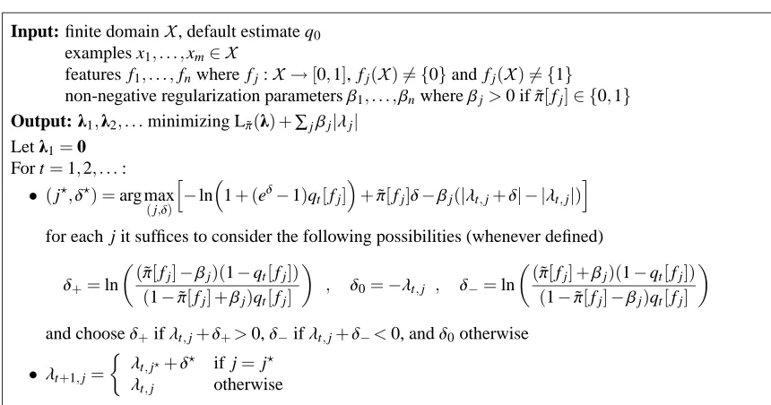
6. Selective-Update Algorithm
In the previous section, we have discussed performance bounds of various types of regularization. Now we turn our attention to algorithms for solving generalized maxent problems. In the present and the following section, we propose two algorithms for generalized maxent with complete proofs of convergence. Our algorithms cover a wide class of potentials including the basic, box and `2 2
potential. The`2-ball potential U( √
2) ˜
π does not fall in this class, but we show that the corresponding maxent problem can be reduced and our algorithms can still be applied.
There are a number of algorithms for finding the basic maxent distribution, especially iterative scaling and its variants (Darroch and Ratcliff, 1972; Della Pietra et al., 1997). The Selective-Update algorithm for MaximuM EnTropy (SUMMET) described in this section modifies one weightλj
at a time, as explored by Collins, Schapire, and Singer (2002) in a similar setting. This style of coordinate-wise descent is convenient when working with a very large (or infinite) number of fea-tures. The original Darroch and Ratcliff algorithm also allows single-coordinate updates. Goodman (2002) observes that this leads to a much faster convergence than with the parallel version. However, updates are performed cyclically over all features, which renders the algorithm less practical with a large number of irrelevant features. Similarly, the sequential-update algorithm of Krishnapuram et al. (2005) requires a visitation schedule that updates each feature weight infinitely many times.
SUMMET differs since the weight to be updated is selected independently in each iteration. Thus, the features whose optimal weights are zero may never be updated. This approach is particu-larly useful in the context of`1-regularized maxent which often yields sparse solutions.
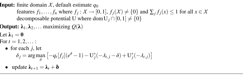
As explained in Section 4, the goal of the algorithm is to produce a sequenceλ1,λ2, . . . maxi-mizing the objective function Q in the limit. In this and the next section we assume that the potential U is decomposable as defined below:
Definition 16. A potential U :Rn→(−∞,∞]is called decomposable if it can be written as a sum of
coordinate potentials U(u) =∑jUj(uj), each of which is a closed proper convex function bounded
from below.