Distributional Word Clusters vs. Words for Text Categorization
Ron Bekkerman [email protected]
Ran El-Yaniv [email protected]
Department of Computer Science Technion - Israel Institute of Technology Haifa 32000, Israel
Naftali Tishby [email protected]
School of Computer Science and Engineering and Center for Neural Computation
The Hebrew University Jerusalem 91904, Israel
Yoad Winter [email protected]
Department of Computer Science Technion - Israel Institute of Technology Haifa 32000, Israel
Editors: Isabelle Guyon and Andr´e Elisseeff
Abstract
We study an approach to text categorization that combines distributional clustering of words and a Support Vector Machine (SVM) classifier. This word-cluster representation is computed using the recently introduced Information Bottleneck method, which generates a compact and efficient rep-resentation of documents. When combined with the classification power of the SVM, this method yields high performance in text categorization. This novel combination of SVM with word-cluster representation is compared with SVM-based categorization using the simpler bag-of-words (BOW) representation. The comparison is performed over three known datasets. On one of these datasets (the 20 Newsgroups) the method based on word clusters significantly outperforms the word-based representation in terms of categorization accuracy or representation efficiency. On the two other sets (Reuters-21578 and WebKB) the word-based representation slightly outperforms the word-cluster representation. We investigate the potential reasons for this behavior and relate it to structural differences between the datasets.
1. Introduction
In this paper we empirically study a familiar representation technique that is based on word-clusters. Our experiments indicate that text categorization based on this representation can outper-form categorization based on the BOW representation, although the peroutper-formance that this method achieves may depend on the chosen dataset. These empirical conclusions about the categoriza-tion performance of word-cluster representacategoriza-tions appear to be new. Specifically, we apply the re-cently introduced Information Bottleneck (IB) clustering framework (Tishby et al., 1999; Slonim and Tishby, 2000, 2001) for generating document representation in a word cluster space (instead of word space), where each cluster is a distribution over document classes. We show that the combina-tion of this IB-based representacombina-tion with a Support Vector Machine (SVM) classifier (Boser et al., 1992; Sch¨olkopf and Smola, 2002) allows for high performance in categorizing three benchmark datasets: 20 Newsgroups (20NG), Reuters-21578 and WebKB. In particular, our categorization of 20NG outperforms the strong algorithmic word-based setup of Dumais et al. (1998) (in terms of cat-egorization accuracy or representation efficiency), which achieved the best reported catcat-egorization results for the 10 largest categories of the Reuters dataset.
This representation using word clusters, where words are viewed as distributions over docu-ment categories, was first suggested by Baker and McCallum (1998) based on the “distributional clustering” idea of Pereira et al. (1993). This technique enjoys a number of intuitively appealing properties and advantages over other feature selection (or generation) techniques. First, the di-mensionality reduction computed by this word clustering implicitly considers correlations between the various features (terms or words). In contrast, popular “filter-based” greedy approaches for feature selection such as Mutual Information, Information Gain and TFIDF (see, e.g., Yang and Pedersen, 1997) only consider each feature individually. Second, the clustering that is achieved by the IB method provides a good solution to the statistical sparseness problem that is prominent in the straightforward word-based (and even more so in n-gram-based) document representations. Third, the clustering of words generates extremely compact representations (with minor information compromises) that enable strong but computationally intensive classifiers. Besides these intuitive advantages, the IB word clustering technique is formally motivated by the Information Bottleneck principle, in which the computation of word clusters aims to optimize a principled target function (see Section 3 for further details).
Despite these conceptual advantages of this word cluster representation and its success in cate-gorizing the 20NG dataset, we show that it does not improve accuracy over BOW-based categoriza-tion, when it is used to categorize the Reuters dataset (ModApte split) and a subset of the WebKB dataset. We analyze this phenomenon and observe that the categories of documents in Reuters and WebKB are less “complex” than the categories of 20NG in the sense that documents can almost be “optimally” categorized using a small number of keywords. This is not the case for 20NG, where the contribution of low frequency words to text categorization is significant.
2. Related Results
In this section we briefly overview results which are most relevant for the present work. Thus, we limit the discussion to relevant feature selection and generation techniques, and best known cate-gorization results over the corpora we consider (Reuters-21578, the 20 Newsgroups and WebKB). For more comprehensive surveys on text categorization the reader is referred to Sebastiani (2002); Singer and Lewis (2000) and references therein. Throughout the discussion we assume familiarity with standard terms used in text categorization.1
We start with a discussion of feature selection and generation techniques. Dumais et al. (1998) report on experiments with multi-labeled categorization of the Reuters dataset. Over a BOW binary representation (where each word receives a count of 1 if it occurs once or more in a document and 0 otherwise) they applied the Mutual Information index for feature selection. Specifically, let C denote the set of document categories and let Xc∈ {0,1}be a binary random variable denoting the
event that a random document belongs (or not) to category c∈C. Similarly, let Xw∈ {0,1} be a
random variable denoting the event that the word w occurred in a random document. The Mutual Information between Xcand Xwis
I(Xc,Xw) =
∑
Xc,Xw∈{0,1}P(Xc,Xw)log
P(Xc,Xw)
P(Xc)P(Xw).
(1)
Note that when evaluating I(Xc,Xw)from a sample of documents, we compute P(Xc,Xw), P(Xc)and
P(Xw)using their empirical estimates.2 For each category c, all the words are sorted according to
decreasing value of I(Xc,Xw)and the k top scored words are kept, where k is a pre-specified or
data-dependent parameter. Thus, for each category there is a specialized representation of documents projected to the most discriminative words for the category.3 In the sequel we refer to this Mutual Information feature selection technique as “MI feature selection” or simply as “MI”.
Dumais et al. (1998) show that together with a Support Vector Machine (SVM) classifier, this MI feature selection method yields a 92.0% break-even point (BEP) on the 10 largest categories in the Reuters dataset.4 As far as we know this is the best multi-labeled categorization result of the (10 largest categories of the) Reuters dataset. Therefore, in this work we consider the SVM classifier with MI feature selection as a baseline for handling BOW-based categorization. Some other recent works also provide strong evidence that SVM is among the best classifiers for text categorization. Among these works it is worth mentioning the empirical study by Yang and Liu (1999) (who showed that SVM outperforms other classifiers, including kNN and Naive Bayes, on Reuters with both large and small training sets) and the theoretical account of Joachims (2001) for the suitability of SVM for text categorization.
1. Specifically, we refer to precision/recall-based performance measures such as break-even-point (BEP) and F-measure and to uni-labeled and multi-labeled categorization. See Section 5.1 for further details.
2. Consider, for instance, Xc=1 and Xw=1. Then P(Xc,Xw) =NNw((cc)), P(Xc) =NN(c), P(Xw) =NNw, where Nw(c)is a
number of occurrences of word w in category c, N(c)is the total number of words in c, Nwis a number of occurrences
of word w in all the categories, and N is the total number of words.
3. Note that throughout the paper we consider categorization schemes that decompose m-category categorization prob-lems into m binary probprob-lems in a standard “one-against-all” fashion. Other decompositions based on error correcting codes are also possible; see (Allwein et al., 2000) for further details.
Baker and McCallum (1998) apply the distributional clustering scheme of Pereira et al. (1993) (see Section 3) for clustering words represented as distributions over categories of the documents where they appear. Given a set of categories
C
={ci}mi=1, a distribution of a word w over the categories is {P(ci|w)}mi=1. Then the words (represented as distributions) are clustered using an agglomerative clustering algorithm. Using a naive Bayes classifier (operated on these conditional distributions) the authors tested this method for uni-labeled categorization of the 20NG dataset and reported an 85.7% accuracy. They also compare this word cluster representation to other feature selection and generation techniques such as Latent Semantic Indexing (see, e.g., Deerwester et al., 1990), the above Mutual Information index and the Markov “blankets” feature selection technique of Koller and Sahami (1996). The authors conclude that categorization that is based on word clus-ters is slightly less accurate than the other methods while keeping a significantly more compact representation.The “distributional clustering” approach of Pereira et al. (1993) is a special case of the general Information Bottleneck (IB) clustering framework presented by Tishby et al. (1999); see Section 3.1 for further details. Slonim and Tishby (2001) further study the power of this distributional word clusters representation and motivate it within the more general IB framework (Slonim and Tishby, 2000). They show that categorization based on this representation can improve the accuracy over the BOW representation whenever the training set is small (about 10 documents per category). Specifically, using a Naive Bayes classifier on a dataset consisting of 10 categories of 20NG, they observe 18.4% improvement in accuracy over a BOW-based categorization.
Joachims (1998b) used an SVM classifier for a multi-labeled categorization of Reuters without feature selection, and achieved a break-even point of 86.4%. Joachims (1997) also investigates uni-labeled categorization of the 20NG dataset, and applies the Rocchio classifier (Rocchio, 1971) over TFIDF-weighted (see, e.g., Manning and Sch¨utze, 1999) BOW representation that is reduced using the Mutual Information index. He obtains 90.3% accuracy, which to-date is, to our knowledge, the best published accuracy of a uni-labeled categorization of the 20NG dataset. Joachims (1999) also experiments with SVM categorization of the WebKB dataset (see details of these results in the last row in Table 1).
Schapire and Singer (1998) consider text categorization using a variant of AdaBoost (Freund and Schapire, 1996) applied with one-level decision trees (also known as decision stamps) as the base classifiers. The resulting algorithm, called BoosTexter, achieves 86.0% BEP on all the categories of Reuters (ModApte split). Weiss et al. (1999) also employ boosting (using decision trees as the base classifiers and an adaptive resampling scheme). They categorize Reuters (ModApte split) with 87.8% BEP using the largest 95 categories (each having at least 2 training examples). To our knowledge this is the best result that has been achieved on (almost) the entire Reuters dataset.
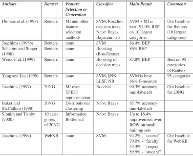
Table 1 summarizes the results that were discussed in this section.
3. Methods and Algorithms
Authors Dataset Feature Classifier Main Result Comments Selection or
Generation
Dumais et al. (1998) Reuters MI and other SVM, Rocchio, SVM + MI is Our baseline feature decision trees, best: 92.0% BEP for Reuters selection Naive Bayes, on 10 largest (10 largest
methods Bayesian nets categories categories)
Joachims (1998b) Reuters none SVM 86.4% BEP
Schapire and Singer Reuters none Boosting 86% BEP
(1998) (BoosTexter)
Weiss et al. (1999) Reuters none Boosting of 87.8% BEP Best on 95
decision trees categories
of Reuters
Yang and Liu (1999) Reuters none SVM, kNN, SVM is best: 95 categories
LLSF, NB 86% F-measure
Joachims (1997) 20NG MI over Rocchio 90.3% accuracy Our baseline
TFIDF (uni-labeled) for 20NG
representation
Baker and 20NG Distributional Naive Bayes 85.7% accuracy
McCallum (1998) clustering (uni-labeled)
Slonim and Tishby 10 cate- Information Naive Bayes Up to 18.4%
(2000) gories Bottleneck improvement over
of 20NG BOW on small
training sets
Joachims (1999) WebKB none SVM 94.2% - “course” Our baseline
79.0% - “faculty” for WebKB 53.3% - “project”
89.9% - “student”
Table 1: Summary of related results.
3.1 Information Bottleneck and Distributional Clustering
Data clustering is a challenging task in information processing and pattern recognition. The chal-lenge is both conceptual and computational. Intuitively, when we attempt to cluster a dataset, our goal is to partition it into subsets such that points in the same subset are more “similar” to each other than to points in other subsets. Common clustering algorithms depend on choosing a similarity mea-sure between data points and a “correct” clustering result can be dependent on an appropriate choice of a similarity measure. The choice of a “correct” measure must be defined relative to a particular application. For instance, consider a hypothetical dataset containing articles by each of two authors, so that half of the articles authored by each author discusses one topic, and the other half discusses another topic. There are two possible dichotomies of the data which could yield two different bi-partitions: according to the topic or according to the writing style. When asked to cluster this set into two sub-clusters, one cannot successfully achieve the task without knowing the goal. Therefore, without a suitable target at hand and a principled method for choosing a similarity measure suitable for the target, it can be meaningless to interpret clustering results.
the IB method aims to construct a relevant encoding of the random variable X by partitioning X into domains that preserve (as much as possible) the Mutual Information between X and another “relevance” variable, Y . The relation between X and Y is made known via i.i.d. observations from the joint distribution P(X,Y). Denote the desired partition (clustering) of X by ˜X . We determine ˜X by solving the following variational problem: Maximize the Mutual Information I(X˜,Y)with respect to the partition P(X˜|X), under a minimizing constraint on I(X˜,X). In particular, the Information Bottleneck method considers the following optimization problem: Maximize
I(X˜,Y)−βI(X˜,X)
over the conditional P(X˜|X), where the parameter β determines the allowed amount of reduction in information that ˜X bears on X . Namely, we attempt to find the optimal tradeoff between the minimal partition of X and the maximum preserved information on Y . Tishby et al. (1999) show that a solution for this optimization problem is characterized by
P(X˜|X) = P(X˜) Z(β,X)exp
"
−β
∑
YP(Y|X)ln
P(Y|X) P(Y|X˜)
# ,
where Z(β,X)is a normalization factor, and P(Y|X˜)in the exponential is defined implicitly, through Bayes’ rule, in terms of the partition (assignment) rules P(X˜|X), P(Y|X˜) =P(1X˜)∑XP(Y|X)P(X˜|X)P(X) (see Tishby et al., 1999, for details). The parameterβis a Lagrange multiplier introduced for the constrained information, but using a thermodynamical analogyβcan also be viewed as an inverse temperature, and can be utilized as an annealing parameter to choose a desired cluster resolution.
Before we continue and present the IB clustering algorithm in the next section, we note on the contextual background of the IB method and its connection to “distributional clustering”. Pereira, Tishby, and Lee (1993) introduced “distributional clustering” for distributions of verb-object pairs. Their algorithm clustered nouns represented as distributions over co-located verbs (or verbs repre-sented as distributions over co-located nouns). This clustering routine aimed at minimizing the av-erage distributional similarity (in terms of the Kullback-Leibler divergence, see Cover and Thomas, 1991) between the conditional P(verb|noun)and the noun centroid distributions (i.e. these centroids are also distributions over verbs). It turned out that this routine is a special case of the more gen-eral IB framework. IB clustering has since been used to derive a variety of effective clustering and categorization routines (see, e.g., Slonim and Tishby, 2001; El-Yaniv and Souroujon, 2001; Slonim et al., 2002) and has interesting extensions (Friedman et al., 2001; Chechik and Tishby, 2002). We note also that unlike other variants of distributional clustering (such as the PLSI approach of Hoff-man, 2001), the IB method is not based on a generative (mixture) modelling approach (including their assumptions) and is therefore more robust.
3.2 Distributional Clustering via Deterministic Annealing
Given the IB Markov chain condition ˜X ↔X ↔Y (which is not an assumption on the data; see Tishby et al., 1999, for details), a solution to the IB optimization satisfies the following self-consistent equations:
P(X˜|X) = P(X˜) Z(β,X)exp
"
−β
∑
YP(Y|X)ln
P(Y|X) P(Y|X˜)
#
P(X˜) =
∑
X
P(X)P(X˜|X); (3)
P(Y|X˜) =
∑
X
P(Y|X)P(X|X˜). (4)
Tishby et al. (1999) show that a solution can be obtained by starting with an arbitrary solution and then iterating the equations. For any value of β this procedure is guaranteed to converge.5 Lower values of theβparameter (high “temperatures”) correspond to poor distributional resolution (i.e. fewer clusters) and higher values ofβ(low “temperatures”) correspond to higher resolutions (i.e. more clusters).
Input:
P(X,Y)- Observed joint distribution of two random variables X and Y
k - desired number of centroids
βmin,βmax- minimal / maximal values ofβ
ν>1 - annealing rate
δconv>0 - convergence threshold,δmerge>0 - merging threshold Output:
Cluster centroids, given by{P(Y|˜xi)}ki=1
Cluster assignment probabilities, given by P(X˜|X)
Initiateβ←βmin- currentβparameter Initiate r←1 - current number of centroids repeat
{1. “EM”-like iteration:}
Compute P(X˜|X), P(X˜)and P(Y|X˜)using Equations (2), (3) and (4) respectively repeat
Let Pold(X˜|X)←P(X˜|X)
Compute new values for P(X˜|X), P(X˜)and P(Y|X˜)using (2), (3) and (4) until for each x:kP(X˜|x)−Pold(X˜|x)k<δconv
{2. Merging:}
for all i,j∈[1,r]s.t. i<j andkP(Y|x˜i)−P(Y|x˜j)k<δmergedo
Merge ˜xiand ˜xj: P(x˜i|X) =P(x˜i|X) +P(x˜j|X)
Let r←r−1 end for
{3. Centroid ghosting:} for all i∈[1,r]do
Create ˜xr+is.t.kP(Y|x˜r+i)−P(Y|x˜i)k=δmerge
Let P(x˜i|X)←21P(x˜i|X), P(x˜r+i|X)←21P(x˜i|X)
end for
Let r←2r,β←νβ until r>k orβ>βmax
If r>k then merge r−k closest centroids (each to its closest centroid neighbor)
Algorithm 1: Information Bottleneck distributional clustering
We use a hierarchical top-down clustering procedure for recovering the distributional IB clus-ters. A pseudo-code of the algorithm is given in Algorithm 1.6 Starting with one cluster (very small β) that contains all the data we incrementally achieve the desired number of clusters by performing a process consisting of annealing stages. At each annealing stage we incrementβand attempt to
5. This procedure is analogous to the Blahut-Arimoto algorithm in Information Theory (Cover and Thomas, 1991). 6. A similar annealing procedure, known as deterministic annealing, was introduced in the context of clustering by
split existing clusters. This is done by creating (for each centroid) a new “ghost” centroid at some random small distance from the original centroid. We then attempt to cluster the points (distribu-tions) using all (original and ghost) centroids by iterating the above IB self-consisting equations, similar to the Expectation-Maximization (EM) algorithm (Dempster et al., 1977). During these iter-ations the centroids are adjusted to their (locally) optimal positions and (depending on the annealing increment ofβ) some “ghost” centroids can merge back with their centroid sources. Note that in this scheme (as well as in the similar deterministic annealing algorithm of Rose, 1998), one has to use an appropriate annealing rate in order to identify phase transitions which correspond to cluster splits.
An alternative agglomerative (bottom-up) hard-clustering IB algorithm was developed by Slonim and Tishby (2000). This algorithm generates hard clustering of the data and thus approximates the above IB clustering procedure. Note that the time complexity of this algorithm is O(n2), where n is the number of data points (distributions) to be clustered (see also an approximate faster agglomera-tive procedure by Baker and McCallum, 1998).
The application of the IB clustering algorithm in our context is straightforward. The variable X represents words that appear in training documents. The variable Y represents class labels and thus, the joint distribution P(X,Y)is characterized by pairs(w,c), where w is a word and c is the class label of the document where w appears. Starting with the observed conditionals{P(Y =c|X=w)}c
(giving for each word w its class distribution) we cluster these distributions using Algorithm 1. For a pre-specified number of clusters k the output of Algorithm 1 is: (i) k centroids, given by the distributions{P(X˜ =w˜|X =w)}w˜ for each word w, where ˜w are the word centroids (i.e. there are
k such word centroids which represent k word clusters); (ii) Cluster assignment probabilities given by P(X˜|X). Thus, each word w may (partially) belong to all k clusters and the association weight of w to the cluster represented by the centroid ˜w is P(w˜|w).
The time complexity of Algorithm 1 is O(c1c2mn), where c1 is an upper limit on the number of annealing stages, c2 is an upper limit on the number of convergence stages, m is the number of categories and n is the number of data points to cluster.
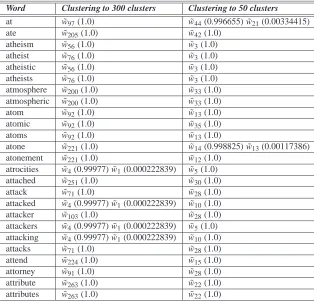
In Table 2 we provide an example of the output of Algorithm 1 applied to the 20NG cor-pus (see Section 4.2) with both k=300 and k=50 cluster centroids. For instance, we see that P(w˜4|attacking)=0.99977 and P(w˜1|attacking) =0.000222839. Thus, the word “attacking” mainly belongs to cluster ˜w4. As can be seen, all the words in the table belong to a single cluster or mainly to a single cluster. With values of k in this range this behavior is typical to most of the words in this corpus (the same is also true for the Reuters and WebKB datasets). Only a small fraction of less than 10% of words significantly belong to more than one cluster, for any number of clusters 506k6500. It is also interesting to note that IB clustering often results in word stemming. For in-stance, “atom” and “atoms” belong to the same cluster. Moreover, contextually synonymous words are often assigned to the same cluster. For instance, many “computer words” such as “computer”, “hardware”, “ibm”, “multimedia”, “pc”, “processor”, “software”, “8086” etc. compose the bulk of one cluster.
3.3 Support Vector Machines (SVMs)
Word Clustering to 300 clusters Clustering to 50 clusters
at w˜97(1.0) w˜44(0.996655) ˜w21(0.00334415)
ate w˜205(1.0) w˜42(1.0)
atheism w˜56(1.0) w˜3(1.0)
atheist w˜76(1.0) w˜3(1.0)
atheistic w˜56(1.0) w˜3(1.0)
atheists w˜76(1.0) w˜3(1.0)
atmosphere w˜200(1.0) w˜33(1.0)
atmospheric w˜200(1.0) w˜33(1.0)
atom w˜92(1.0) w˜13(1.0)
atomic w˜92(1.0) w˜35(1.0)
atoms w˜92(1.0) w˜13(1.0)
atone w˜221(1.0) w˜14(0.998825) ˜w13(0.00117386)
atonement w˜221(1.0) w˜12(1.0)
atrocities w˜4(0.99977) ˜w1(0.000222839) w˜5(1.0)
attached w˜251(1.0) w˜30(1.0)
attack w˜71(1.0) w˜28(1.0)
attacked w˜4(0.99977) ˜w1(0.000222839) w˜10(1.0)
attacker w˜103(1.0) w˜28(1.0)
attackers w˜4(0.99977) ˜w1(0.000222839) w˜5(1.0) attacking w˜4(0.99977) ˜w1(0.000222839) w˜10(1.0)
attacks w˜71(1.0) w˜28(1.0)
attend w˜224(1.0) w˜15(1.0)
attorney w˜91(1.0) w˜28(1.0)
attribute w˜263(1.0) w˜22(1.0)
attributes w˜263(1.0) w˜22(1.0)
Table 2: A clustering example of 20NG words. ˜wi are centroids to which the words “belong”, the
centroid weights are shown in the brackets.
Section 2 there is much empirical support for using SVMs for text categorization (Joachims, 2001; Dumais et al., 1998, etc.).
Informally, for linearly separable two-class data, the (linear) SVM computes the maximum mar-gin hyperplane that separates the classes. For non-linearly separable data there are two possible extensions. The first (Cortes and Vapnik, 1995) computes a “soft” maximum margin separating hyperplane that allows for training errors. The accommodation of errors is controlled using a fixed cost parameter. The second solution is obtained by implicitly embedding the data into a high (or infinite) dimensional space where the data is likely to be separable. Then, a maximum margin hy-perplane is sought in this high-dimensional space. A combination of both approaches (soft margin and embedding) is often used.
SVMs are well covered by numerous papers, books and tutorials and therefore we suppress further descriptions here. Following Joachims (2001) and Dumais et al. (1998) we use a linear SVM in all our experiments. The implementation we use is SVMlight of Joachims.7
3.4 Putting it All Together
For handling m-class categorization problems (m>2) we choose (for both the uni-labeled and multi-labeled settings) a straightforward decomposition into m binary problems. Although this de-composition is not the best for all datasets (see, e.g., Allwein et al., 2000; F ¨urnkranz, 2002) it allows for a direct comparison with the related results (which were all achieved using this decom-position as well, see Section 2). Thus, for a categorization problem into m classes we construct m binary classifiers such that each classifier is trained to distinguish one category from the rest. In multi-labeled categorization (see Section 5.1) experiments we construct for each category a “hard” (threshold) binary SVM and each test document is considered by all binary classifiers. The subset of categories attributed for this document is determined by the subset of classifiers that “accepted” it. On the other hand, in uni-labeled experiments we construct for each category a confidence-rated SVM that output for a (test) document a real confidence-rate based on the distance of the point to the decision hyperplane. The (single) category of a test document is determined by the classifier that outputs the largest confidence rate (this approach is sometimes called “max-win”).
A major goal of our work is to compare two categorization schemes based on the two rep-resentations: the simple BOW representation together with Mutual Information feature selection (called here BOW+MI) and a representation based on word clusters computed via IB distributional clustering (called here IB).
We first consider a BOW+MI uni-labeled categorization. Given a training set of documents in m categories, for each category c, a binary confidence-rated linear SVM classifier is trained using the following procedure: The k most discriminating words are selected according to the Mutual Information between the word w and the category c (see Equation (1)). Then each training document of category c is projected over the corresponding k “best” words and for each category c a dedicated classifier hcis trained to separate c from the other categories. For categorizing a new (test) document
d, for each category c we project d over the k most discriminating words of category c. Denoting a projected document d by dc, we compute hc(dc)for all categories c. The category attributed for d
is arg maxchc(dc). For multi-labeled categorization the same procedure is applied except that now
we train, for each category c, hard (non-confidence-rated) classifiers hcand the subset of categories
attributed for a test document d is{c : hc(dc) =1}.
The structure of the IB categorization scheme is similar (in both the uni-labeled and multi-labeled settings) but now the representation of a document consists of vectors of word cluster counts corresponding to a cluster mapping (from words to cluster centroids) that is computed for all categories simultaneously using the Information Bottleneck distributional clustering procedure (Algorithm 1).
4. Datasets
Three benchmark datasets - Reuters-21578, 20 Newsgroups and WebKB - were experimented with in our application of feature selection for text categorization. In this section we describe these datasets and the preprocessing that was applied to them.
4.1 Reuters-21578
The Reuters-21578 corpus contains 21578 articles taken from the Reuters newswire.8 Each article is typically designated into one or more semantic categories such as “earn”, “trade”, “corn” etc., where the total number of categories is 114. We used the ModApte split, which consists of a training set of 7063 articles and a test set of 2742 articles.9
In both the training and test sets we preprocessed each article so that any additional information except for the title and the body was removed. In addition, we lowered the case of letters. Following Dumais et al. (1998) we generated distinct features for words that appear in article titles. In the IB-based setup (see Section 3.4) we applied a filter on low-frequency words: we removed words that appear in Wlow f req articles or less, where Wlow f req is determined using cross-validation (see
Section 5.2). In the BOW+MI setup this filtering of low-frequency words is essentially not relevant since these words are already filtered out by the Mutual Information feature selection index.
4.2 20 Newsgroups
The 20 Newsgroups (20NG) corpus contains 19997 articles taken from the Usenet newsgroups collection.10 Each article is designated into one or more semantic categories and the total number of categories is 20, all of them are of about the same size. Most of the articles have only one semantic label, while about 4.5% of the articles have two or more labels. Following Schapire and Singer (2000) we used the “Xrefs” field of the article headers to detect multi-labeled documents and to remove duplications. We preprocessed each article so that any additional information except for the subject and the body was removed. In addition, we filtered out lines that seemed to be part of binary files sent as attachments or pseudo-graphical text delimiters. A line is considered to be a “binary” (or a delimiter) if it is longer than 50 symbols and contains no blanks. Overall we removed 23057 such lines (where most of these occurrences appeared in a dozen of articles overall). Also, we lowered the case of letters. As in the Reuters dataset, in the IB-based setup we applied a filter on low-frequency words, using the parameter Wlow f req determined via cross-validation.
4.3 WebKB: World Wide Knowledge Base
The World Wide Knowledge Base dataset (WebKB)11is a collection of 8282 web pages obtained from four academic domains. The WebKB was collected by Craven et al. (1998). The web pages in the WebKB set are labeled using two different polychotomies. The first is according to topic and the second is according to web domain. In our experiments we only considered the first
poly-8. Reuters-21578 can be found at: http://www.daviddlewis.com/resources/testcollections/reuters21578/.
9. Note that in these figures we count documents with at least one label. The original split contains 9603 training documents and 3299 test documents where the additional articles have no labels. While in practice it may be possible to utilize additional unlabeled documents for improving performance using semi-supervised learning algorithms (see, e.g., El-Yaniv and Souroujon, 2001), in this work we simply discarded these documents.
chotomy, which consists of 7 categories: course, department, faculty, project, staff, student and other. Following Nigam et al. (1998) we discarded the categories other,12 department and staff. The remaining part of the corpus contains 4199 documents in four categories. Table 3 specifies the 4 remaining categories and their sizes.
Category Number of articles Proportion (%)
course 930 22.1
faculty 1124 26.8
project 504 12.0
student 1641 39.1
Table 3: Some essential details of WebKB categories.
Since the web pages are in HTML format, they contain much non-textual information: HTML tags, links etc. We did not filter this information because some of it is useful for categorization. For instance, in some documents anchor-texts of URLs are the only discriminative textual information. We did however filter out non-literals and lowered the case of letters. As in the other datasets, in the IB-based setup we applied a filter on low-frequency words, using the parameter Wlow f req
(determined via cross-validation).
5. Experimental Setup
This section presents our experimental model, starting with a short overview of the evaluation meth-ods we used.
5.1 Optimality Criteria and Performance Evaluation
We are given a training set
D
train={(d1,`1),...,(dn,`n)} of labeled text documents, where eachdocument di belongs to a document set
D
and the label`i=`i(di)of di is within a predefined setof categories
C
={c1,...,cm}. In the multi-labeled version of text categorization, a document canbelong to several classes simultaneously. That is, both h(d)and`(d)can be sets of categories rather than single categories. In the case where each document has only a single label we say that the categorization is uni-labeled.
We measure the empirical effectiveness of multi-labeled text categorization in terms of the clas-sical information retrieval parameters of “precision” and “recall” (Baeza-Yates and Ribeiro-Neto, 1999). Consider a multi-labeled categorization problem with m classes,
C
={c1,...,cm}. Let h bea classifier that was trained for this problem. For a document d, let h(d)⊆
C
be the set of categories designated by h for d. Let`(d)⊆C
be true categories of d. LetD
test⊂D
be a test set of “unseen”documents that were not used in the construction of h. For each category ci, define the following
quantities:
T Pi =
∑
d∈Dtest
I[ci∈`(d)∧ci∈h(d)],
T Ni =
∑
d∈Dtest
I[ci∈`(d)∧ci6∈h(d)],
FPi =
∑
d∈DtestI[ci6∈`(d)∧ci∈h(d)],
where I[·]is the indicator function. For example, F Pi(the “false positives” with respect to ci) is the
number of documents categorized by h into ci whose true set of labels does not include ci, etc. For
each category ci we now define the precision Pi=Pi(h)of h and the recall Ri=Ri(h)with respect
to ci as Pi=T PT Pi+FPi i and Ri=T PT Pi+T Ni i. The overall micro-averaged precision P=P(h)and recall
R=R(h)of h is a weighted average of the individual precisions and recalls (weighted with respect to the sizes of the test set categories). That is, P= ∑mi=1T Pi
∑m
i=1(T Pi+FPi) and R=
∑m i=1T Pi
∑m
i=1(T Pi+T Ni). Due to the natural tradeoff between precision and recall, the following two quantities are often used in order to measure the performance of a classifier:
• F-measure: The harmonic mean of precision and recall; that is F=1/P+21/R.
• Break-Even Point (BEP): A flexible classifier provides the means to control the tradeoff be-tween precision and recall. For such classifiers, the value of P (and R) satisfying P=R is called the break-even point (BEP). Since it is time consuming to evaluate the exact value of the BEP it is customary to estimate it using the arithmetic mean of P and R.
The above performance measures concern multi-labeled categorization. In a uni-labeled categoriza-tion the accepted performance measure is accuracy, defined to be the percentage of correctly labeled documents in
D
test. Specifically, assuming that both h(d)and`(d)are singletons (i.e. uni-labeling),the accuracy Acc(h) of h is Acc(h) = |D1
test|∑d∈DtestI[h(d) =`(d)]. Is it not hard to see that in this case the accuracy equals the precision and recall (and the estimated break-even point).
Following Dumais et al. (1998) (and for comparison with this work), in our multi-labeled ex-periments (Reuters and 20NG) we report on micro-averaged break-even point (BEP) results. In our uni-labeled experiments (20NG and WebKB) we report on accuracy. Note that we experiment with both uni-labeled and multi-labeled categorization of 20NG. Although this set is in general multi-labeled, the proportion of multi-labeled articles in the dataset is rather small (about 4.5%) and therefore a uni-labeled categorization of this set is also meaningful. To this end, we follow Joachims (1997) and consider our (uni-labeled) categorization of a test document to be correct if the label we assign to the document belongs to its true set of labels.
In order to better estimate the performance of our algorithms on test documents we use standard cross-validation estimation in our experiments with 20NG and WebKB. However, when experi-menting with Reuters, for compatibility with the experiments of Dumais et al. we use its standard ModApte split (i.e. without cross-validation). In particular, in both 20NG and WebKB we use 4-fold cross-validation where we randomly and uniformly split each category into 4 4-folds and we took three folds for training and one fold for testing. Note that this 3/4:1/4 split is proportional to the training to test set size ratios of the ModApte split of Reuters. In the cross-validated experiments we always report on the estimated average (over the 4 folds) performance (either BEP or accuracy), estimated standard deviation and standard error of the mean.
5.2 Hyperparameter Optimization
error and margin) and J (cost-factor, by which training errors on positive examples outweigh er-rors on negative examples). We optimize these parameters using a validation set that consists one third of the three-fold training set.13 For each of these parameters we fix a small set of feasible values14 and in general, we attempt to test performance (over the validation set) using all possible combinations of parameter values over the feasible sets.
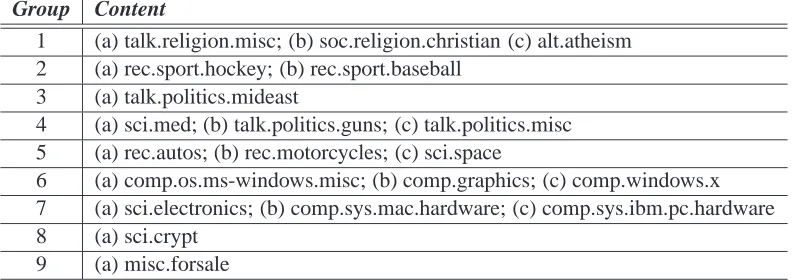
Note that tuning the parameters C and J is different in the multi-labeled and uni-labeled settings. In the multi-labeled setting we tune the parameters of each individual (binary) classifier indepen-dently of the other classifiers. In the uni-labeled setting, parameter tuning is more complex. Since we use the max-win decomposition, the categorization of a document is dependent on all the binary classifiers involved. For instance, if all the classifiers except for one are perfect, this last bad classi-fier can generate confidence rates that are maximal for all the documents, which results in extremely poor performance. Therefore, a global tuning of all the binary classifiers is necessary. Neverthe-less, in the case of the 20NG, where we have 20 binary classifiers, a global exhaustive search is too time-consuming and, ideally, a clever search in this high dimensional parameter space should be considered. Instead, we simply used the information we have on the 20NG categories to reduce the size of the parameter space. Specifically, among the 20 categories of 20NG there are some highly correlated ones and we split the list of the categories into 9 groups as in Table 4.15 For each group the parameters are tuned together and independently of other groups. This way we achieve an ap-proximately global parameter tuning also on the 20NG set. Note that the (much) smaller size of WebKB (both number of categories and number of documents) allow for global parameter tuning over the feasible parameter value sets without any need for approximation.
Group Content
1 (a) talk.religion.misc; (b) soc.religion.christian (c) alt.atheism 2 (a) rec.sport.hockey; (b) rec.sport.baseball
3 (a) talk.politics.mideast
4 (a) sci.med; (b) talk.politics.guns; (c) talk.politics.misc 5 (a) rec.autos; (b) rec.motorcycles; (c) sci.space
6 (a) comp.os.ms-windows.misc; (b) comp.graphics; (c) comp.windows.x 7 (a) sci.electronics; (b) comp.sys.mac.hardware; (c) comp.sys.ibm.pc.hardware 8 (a) sci.crypt
9 (a) misc.forsale
Table 4: A split of the 20NG’s categories into thematic groups.
In IB categorization also the parameter Wlow f req (see Section 4), which determines a filter on
low-frequency words, has a significant impact on categorization quality. Therefore, in IB catego-rization we search for both the SVM parameters and Wlow f req. To reduce the time complexity we
employ the following simple search heuristics. We first fix random values of C and J and then, using
13. Dumais et al. (1998) also use a 1/3 random subset of the training set for validated parameter tuning.
14. Specifically, for the C parameter the feasible set is{10−4,10−3,10−2,10−1}and for J it is{0.5,1,2,...,10}. 15. It is important to note that an almost identical split can be computed in a completely unsupervised manner using the
the validation set, we optimize Wlow f req.16 After determining Wlow f req we tune both C and J as
described above.17
5.3 Fair vs. Unfair Parameter Tuning
In our experiments with the BOW+MI and IB categorizers we sometimes perform unfair parameter tuning in which we tune the SVM parameters over the test set (rather than the validation set). If a categorizer A achieves better performance than a categorizer B while B’s parameters were tuned unfairly (and A’s parameters were tuned fairly) then we can get stronger evidence that A performs better than B. In our experiments we sometimes use this technique to accentuate differences between two categorizers.
6. Categorization Results
We compare text categorization results of the IB and BOW+MI settings. For compatibility with the original BOW+MI setting of Dumais et al. (1998), where the number of best discriminating words k is set to 300, we report on results with k=300 for both settings. In addition, we show BOW+MI results with k=15,000, which is an example for a big value of k that led to good categorization results in the tests we performed. We also report on BOW results without applying MI feature selection.
6.1 Multi-Labeled Categorization
Table 5 summarizes the multi-labeled categorization results obtained by the two categorization schemes (BOW+MI and IB) over Reuters (10 largest categories) and 20NG datasets. Note that the 92.0% BEP result for BOW+MI over Reuters was established by Dumais et al. (1998).18 To the best of our knowledge, the 88.6% BEP we obtain on 20NG is the first reported result of a multi-labeled categorization of this dataset. Previous attempts at multi-multi-labeled categorization of this set were performed by Schapire and Singer (2000), but no overall result on the entire set was reported. On 20NG the advantage of the IB categorizer over BOW+MI is striking when k=300 words (and k=300 word clusters) are used. Note that the 77.7% BEP of BOW+MI is obtained using unfair parameter tuning (see Section 5.3). However, this difference does not sustain when we use k=15,000 words. Using this rather large number of words the BOW+MI performance significantly increases to 86.3% (again, using unfair parameter tuning), which taking into account the statistical deviations is similar to the IB BEP performance. The BOW+MI results that are achieved with fair parameter tuning show an increase in the gap between the performance of the two methods. Never-theless, the IB categorizer achieves this BEP performance using only 300 features (word clusters), almost two order of magnitude smaller than 15,000. Thus, with respect to 20NG, the IB categorizer outperforms the BOW+MI categorizer both in BEP performance and in representation efficiency. We also tried other values of the k parameter, where 300<k15,000 and k>15,000. We found
16. The set of feasible Wlow f reqvalues we use is{0,2,4,6,8}.
17. The “optimal” determined value of Wlow f reqfor Reuters is 4, for WebKB (across all folds) it is 8 and for 20NG it
is 0. The number of distinct words after removing low-frequency words is: 9,953 for Reuters (Wlow f req=4), about
110,000 for 20NG (Wlow f req=0) and about 7,000 for WebKB (Wlow f req=8), depending on the fold.
Categorizer Reuters (BEP) 20NG (BEP)
BOW+MI 92.0 76.5±0.4 (0.25)
k=300 obtained by Dumais et al. (1998) 77.7±0.5 (0.31) unfair
BOW+MI 92.0 85.6±0.6 (0.35)
k=15000 86.3±0.5 (0.27) unfair
BOW 89.7 86.5±0.4 (0.26) unfair
IB 91.2 88.6±0.3 (0.21)
k=300 92.6 unfair
Table 5: Multi-labeled categorization BEP results for 20NG and Reuters. k is the number of se-lected words or word-clusters. All 20NG results are averages of 4-fold cross-validation. Standard deviations are given after the “±” symbol and standard errors of the means are given in brackets. “Unfair” indicates unfair parameter tuning over the test sets (see Sec-tion 5.3).
that the learning curve, as a function of k, is monotone increasing until it reaches a plateau around k=15,000.
We repeat the same experiment over the Reuters dataset but there we obtain different results. Now the IB categorizer lose its BEP advantage and achieves a 91.2% BEP,19 a slightly inferior (but quite similar) performance to the BOW+MI categorizer (as reported by Dumais et al., 1998). Note that the BOW+MI categorizer does not benefit from increasing the number of features up to k=15,000. Furthermore, using all features led to a decrease of 2% in BEP.
Categorizer WebKB (Accuracy) 20NG (Accuracy)
BOW+MI 92.6±0.3 (0.20) 84.7±0.7 (0.41)
k=300 85.5±0.7 (0.45) unfair
BOW+MI 92.4±0.5 (0.32) 90.2±0.3 (0.17)
k=15000 90.9±0.2 (0.12) unfair
BOW 92.3±0.5 (0.40) 91.2±0.1 (0.08) unfair IB 89.5±0.7 (0.41) 91.3±0.4 (0.24) k=300 91.0±0.5 (0.32) unfair
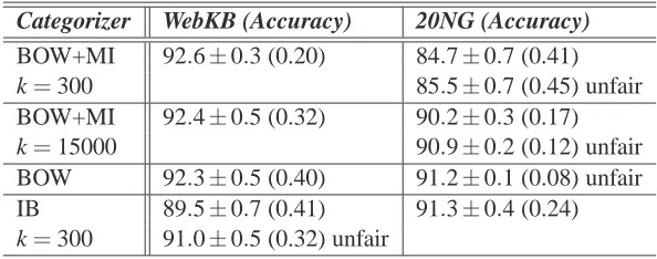
Table 6: Uni-labeled categorization accuracy for 20NG and WebKB. k is the number of selected words or word-clusters. All accuracies are averages of 4-fold cross-validation. Standard deviations are given after the “±” symbol and standard errors of the means are given in brackets. “Unfair” indicates unfair parameter tuning over the test sets (see Section 5.3).
6.2 Uni-Labeled Categorization
We also perform uni-labeled categorization experiments using the BOW+MI and IB categorizers over 20NG and WebKB. The final accuracy results are shown in Table 6. These results appear to be qualitatively similar to the multi-labeled results presented above with WebKB replacing Reuters. Here again, over the 20NG set, the IB categorizer is showing a clear accuracy advantage over BOW+MI with k=300 and this advantage is diminished if we take k=15,000. On the other hand, we observe a comparable (and similar) accuracy of both categorizers over WebKB, and as it is with Reuters, here again the BOW+MI categorizer does not benefit from increasing the feature set size.
The use of k =300 word clusters in the IB categorizer is not necessarily optimal. We also performed this categorization experiment with different values of k ranging from 100 to 1000. The categorization accuracy slightly increases when k moves from 100 to 200, and does not significantly change when k>200.
7. Discussion: Corpora Complexity vs. Representation Efficiency
The categorization results reported above show that the performance of the BOW+MI categorizer and the IB categorizer is sensitive to the dataset being categorized. What makes the performance of these two categorizers different over different datasets? Why does the more sophisticated IB cate-gorizer outperform the BOW+MI catecate-gorizer (with either higher accuracy or better representation efficiency) over 20NG but not over Reuters and WebKB? In this section we study this question and attempt to identify differences between these corpora that can account for this behavior.
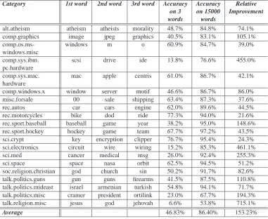
One possible approach to quantify the complexity of a corpus with respect to a categorization system is to observe and analyze learning curves plotting the performance of the categorizer as a function of the number of words selected for representing each category. Before presenting such learning curves for the three corpora, we focus on the extreme case where we categorize each of the corpora using only the three top words per category (where top-scores are measured using the Mutual Information of words with respect to categories). Tables 7, 8 and 9 specify (for each corpus) a list of the top three words for each category, together with the performance achieved by the BOW+MI (binary) classifier of the category. For comparison, we also provide the corresponding performance of BOW+MI using the 15,000 top words (i.e. potentially all the significant words in the corpus). For instance, observing Table 7, computed for Reuters, we see that based only on the words “vs”, “cts” and “loss” it is possible to achieve 93.5% BEP when categorizing the category earn. We note that the word “vs” appears in 87% of the articles of the category earn (i.e., in 914 articles among total 1044 of this category). This word appears in only 15 non-earn articles in the test set and therefore “vs” can, by itself, categorize earn with very high precision.20 This phenomenon was already noticed by Joachims (1997), who noted that a classifier built on only one word (“wheat”) can lead to extremely high accuracy when distinguishing between the Reuters category wheat and the other categories (within a uni-labeled setting).21 The difference between the 20NG and the two other corpora is striking when considering the relative improvement in categorization quality when increasing the feature set up to 15,000 words. While one can dramatically improve categorization
20. In the training set the word “vs” appears in 1900 of the 2709 earn articles (70.1%) and only in 14 of the 4354 non-earn articles (0.3%).
of 20NG by over 150% with many more words, we observe a relative improvement of only about 15% and 26% in the case of Reuters and WebKB, respectively.
1 2 3 4 5 6 7 8 9 10
30 40 50 60 70 80 90
number of features
performance
Reuters 20 newsgroups WebKB
0 50 100 150 200 250 300 30
40 50 60 70 80 90 100
number of features
performance
Reuters 20 newsgroups WebKB
(a) (b)
Figure 1: Learning curves (BEP or accuracy vs. number of words) for the datasets: Reuters-21578 (multi-labeled, BEP), 20NG (uni-labeled, accuracy) and WebKB (uni-labeled, accuracy) over the MI-sorted top 10 words (a) and the top 300 words (b) using the BOW+MI cate-gorizer.
Category 1st word 2nd word 3rd word BEP on BEP on Relative
3 words 15000 words Improvement
earn vs+ cts+ loss+ 93.5% 98.6% 5.4%
acq shares+ vs− Inc+ 76.3% 95.2% 24.7%
money-fx dollar+ vs− exchange+ 53.8% 80.5% 49.6%
grain wheat+ tonnes+ grain+ 77.8% 88.9% 14.2%
crude oil+ bpd+ OPEC+ 73.2% 86.2% 17.4%
trade trade+ vs− cts− 67.1% 76.5% 14.0%
interest rates+ rate+ vs− 57.0% 76.2% 33.6%
ship ships+ vs− strike+ 64.1% 75.4% 17.6%
wheat wheat+ tonnes+ WHEAT+ 87.8% 82.6% -5.9%
corn corn+ tonnes+ vs− 70.3% 83.7% 19.0%
Average 79.9% 92.0% 15.1%
Category 1st word 2nd word 3rd word Accuracy on Accuracy on Relative
3 words 15000 words Improvement
course courses course homework 79.0% 95.7% 21.1%
faculty professor cite pp 70.5% 89.8% 27.3%
project projects umd berkeley 53.2% 80.8% 51.8%
student com uci homes 78.3% 95.9% 22.4%
Average 73.3% 92.4% 26.0%
Table 8: WebKB: Three best words (in terms of Mutual Information) and their categorization ac-curacy rate of the 4 representative categories. All the listed words contribute by their appearance, rather than absence.
Category 1st word 2nd word 3rd word Accuracy Accuracy Relative
on 3 on 15000 Improvement
words words
alt.atheism atheism atheists morality 48.7% 84.8% 74.1%
comp.graphics image jpeg graphics 40.5% 83.1% 105.1%
comp.os.ms- windows m o 60.9% 84.7% 39.0%
windows.misc
comp.sys.ibm. scsi drive ide 13.8% 76.6% 455.0%
pc.hardware
comp.sys.mac. mac apple centris 61.0% 86.7% 42.1%
hardware
comp.windows.x window server motif 46.6% 86.7% 86.0%
misc.forsale 00 sale shipping 63.4% 87.3% 37.6%
rec.autos car cars engine 62.0% 89.6% 44.5%
rec.motorcycles bike dod ride 77.3% 94.0% 21.6%
rec.sport.baseball baseball game year 38.2% 95.0% 148.6%
rec.sport.hockey hockey game team 67.7% 97.2% 43.5%
sci.crypt key encryption clipper 76.7% 95.4% 24.3%
sci.electronics circuit wire wiring 15.2% 85.3% 461.1%
sci.med cancer medical msg 26.0% 92.4% 255.3%
sci.space space nasa orbit 62.5% 94.5% 51.2%
soc.religion.christian god church sin 50.2% 91.7% 82.6%
talk.politics.guns gun guns firearms 41.5% 87.5% 110.8%
talk.politics.mideast israel armenian turkish 54.8% 94.1% 71.7%
talk.politics.misc cramer president ortilink 23.0% 67.7% 194.3%
talk.religion.misc jesus god jehovah 6.6% 53.8% 715.1%
Average 46.83% 86.40% 153.23%
Table 9: 20NG: Three best words (in terms of Mutual Information) and their categorization accu-racy rate (uni-labeled setting). All the listed words contribute by their appearance, rather than absence.
In Figure 1 we present, for each dataset, a learning curve plotting the obtained performance of the BOW+MI categorizer as a function of the number k of selected words.22 As can be seen, the two
curves of both Reuters and WebKB are very similar and almost reach a plateau with k=50 words (that were chosen using the greedy Mutual Information index). This indicates that other words do not contribute much to categorization. But the learning curve of 20NG continues to rise when 0<k<300, and still exhibits a rising slope with k=300 words.
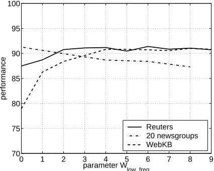
The above findings indicate on a systematic difference between the categorization of the 20NG dataset on the one hand, and of the Reuters and WebKB datasets, on the other hand. We identify another interesting difference between the corpora. This difference is related to the hyper-parameter Wlow f req (see Section 4). The bottom line is that in the case of 20NG IB categorization improves
when Wlow f req decreases while in the case of Reuters and WebKB it improves when Wlow f req
increases. In other words, more words and even the most infrequent words can be useful and improve the (IB) categorization of 20NG. On the other hand, such rare words do add noise in the (IB) categorization of Reuters and WebKB. Figure 2 depicts the performance of the IB classifier on the three corpora as a function of Wlow f req. Note again that this opposite sensitivity to rare words is
observed with respect to the IB scheme and the previous discussion concerns the BOW+MI scheme.
0 1 2 3 4 5 6 7 8 9
70 75 80 85 90 95 100
parameter W low_freq
performance
Reuters 20 newsgroups WebKB
Figure 2: Performance of the IB categorizer as a function of the Wlow f reqparameter (that specifies
the threshold of the low frequency word filter: words appearing in less than Wlow f req
articles are removed); uni-labeled categorization of WebKB and 20NG (accuracy), multi-labeled categorization of Reuters (BEP). Note that Wlow f req=0 corresponds to the case
where this filter is disabled. The number of word clusters in all cases is k=300.
8. Computational Efforts
We performed all our experiments using a 600MHz 2G RAM dual processor Pentium III PC oper-ated by Windows 2000. The IB clustering software, preprocessed datasets and application scripts can be found at:
The computational bottlenecks were mainly experienced over 20NG, which is substantially larger than Reuters and WebKB.
Let us first consider the multi-labeled experiments with 20NG. When running the BOW+MI categorizer, the computational bottleneck was the SVM training, for which a single run (one of the 4 cross-validation folds, including both training and testing) could take a few hours, depending on the parameter values. In general, the smaller the parameters C and J are, the faster the SVM training is.23
As for the IB categorizer, the SVM training process was faster when the input vectors consisted of word clusters. However, the clustering itself could take up to one hour for each fold of the entire 20NG set, and required substantial amount of memory (up to 1G RAM). The overall training and testing time over the entire 20NG in the multi-labeled setting was about 16 hours (4 hours for each of the 4 folds).
The computational bottleneck when running uni-labeled experiments was the SVM parameter tuning. It required a repetition for each combination of the parameters and individual classifiers (see Section 5.2). Overall the experiments with the IB categorizer took about 45 hours of CPU time, while the BOW-MI categorizer required about 96 hours (i.e. 4 days).
The experiments with the relatively small WebKB corpus were accordingly less time-consuming. In particular, the experiments with the SVM+MI categorizer required 7 hours of CPU time and those with the IB categorizer, about 8 hours. Thus, when comparing these times with the experiments on 20NG we see that the IB categorizer is less time-consuming than the BOW+MI categorizer (based on 15000 words) but the clustering algorithm requires larger memory. On Reuters the experiments ran even faster, because there was no need to apply cross-validation estimation.
9. Concluding Remarks
In this study we have provided further evidence for the effectiveness of a sophisticated technique for document representation using distributional clustering of words. Previous studies of distributional clustering of words remained somewhat inconclusive because the overall absolute categorization performance were not state-of-the-art, probably due to the weak classifiers they employed (to the best of our knowledge, in all pervious studies of distributional clustering as a representation method for supervised text categorization, the classifier used was Naive Bayes).
We show that when Information Bottleneck distributional clustering is combined with an SVM classifier, it yields high performance (uni-labeled and multi-labeled) categorization of the three benchmark datasets. In particular, on the 20NG dataset, with respect to either multi-labeled or uni-labeled categorization, we obtain either accuracy (BEP) or representation efficiency advantages over BOW when the categorization is based on SVM. This result indicates that sophisticated document representations can significantly outperform the standard BOW representation and achieve state-of-the-art performance.
Nevertheless, we found no accuracy (BEP) or representation efficiency advantage to this feature generation technique when categorizing the Reuters or WebKB corpora. Our study of the three cor-pora shows structural differences between them. Specifically, we observe that Reuters and WebKB can be categorized with close to “optimal” performance using a small set of words, where the ad-dition of many thousands more words provides no significant improvement. On the other hand, the categorization of 20NG can significantly benefit from the use of a large vocabulary. This indicates
that the “complexity” of the 20NG corpus is in some sense higher than that of Reuters and WebKB. In addition, we see that the IB representation can benefit from including even the most infrequent words when it is applied with the 20NG corpus. On the other hand, such infrequent words do not af-fect or even degrade the performance of the IB categorizer when applied to the Reuters and WebKB corpora.
Based on our experience with the above corpora we note that when testing complex feature selection or generation techniques for text categorization, one should avoid making definitive con-clusions based only on “low-complexity” corpora such as Reuters and WebKB. It seems that so-phisticated representation methods cannot outperform BOW on such corpora.
Let us conclude with some questions and directions for future research. Given a pool of two or more representation techniques and given a corpus, an interesting question is whether it is possible to combine them in a way that will be competitive with or even outperform the best technique in the pool. A straightforward approach would be to perform cross-validated model selection. However, this approach will be at best as good as the best technique in the pool. Another possibility is to try to combine the representation techniques by devising a specialized categorizer for each representation and then use ensemble techniques to aggregate decisions. Other sophisticated approaches such as “co-training” (see, e.g., Blum and Mitchell, 1998) can also be considered.
Our application of the IB distributional clustering of words employed document class labels but generated a global clustering for all categories. Another possibility to consider is to generate specialized clustering for each (binary) classifier. Another interesting possibility to try is to combine clustering of n-grams, with 16n6N for some small N.
Another interesting question that we did not explore concerns the behavior of IB and BOW representations when using feature sets of small cardinality (e.g. k=10). It is expected that at least in “complex” datasets like 20NG, there should be an advantage to the IB representation also in this case.
The BOW+MI categorization employed Mutual Information feature selection, where the num-ber k of features (words) was identical for all categories. It would be interesting to consider a specialized k for each category. Although it might be hard to identify good set of vocabularies, this approach may lead to somewhat better categorization and is likely to generate more efficient representations.
In all our experiments we used the simple-minded one-against-all decomposition technique. It would be interesting to study other decompositions (perhaps, using error correcting output coding approaches). The inter-relation between feature selection/generation and the particular decomposi-tion is of particular importance and may improve text categorizadecomposi-tion performance.
We computed our word clustering using the original top-down (soft) clustering IB implemen-tation of Tishby et al. (1999). It would be interesting to explore the power of more recent IB implementations in this context. Specifically, the IB clustering methods described by El-Yaniv and Souroujon (2001) and Slonim et al. (2002) may yield better clustering in the sense that they tend to better approximate the optimal IB objective.
Acknowledgements
Ravid, Yoram Singer, Noam Slonim and Tong Zhang for their prompt responses and for fruitful discussions. Ran El-Yaniv is a Marcella S. Gelltman Academic Lecturer. A preliminary version of this work appeared at SIGIR 2001.
References
E. L. Allwein, R. E. Schapire, and Y. Singer. Reducing multiclass to binary: A unifying approach for margin classifiers. In Proceedings of ICML’00, 17th International Conference on Machine Learning, pages 9–16. Morgan Kaufmann Publishers, San Francisco, CA, 2000.
R. Baeza-Yates and B. Ribeiro-Neto. Modern Information Retrieval. Addison-Wesley and ACM Press, 1999.
L.D. Baker and A.K. McCallum. Distributional clustering of words for text classification. In Pro-ceedings of SIGIR’98, 21st ACM International Conference on Research and Development in Information Retrieval, pages 96–103, Melbourne, AU, 1998. ACM Press, New York, US.
R. Basili, A. Moschitti, and M.T. Pazienza. Language-sensitive text classification. In Proceedings of RIAO’00, 6th International Conference “Recherche d’Information Assistee par Ordinateur”, pages 331–343, Paris, France, 2000.
A. Blum and T. Mitchell. Combining labeled and unlabeled data with co-training. In COLT’98: Pro-ceedings of 11th Annual Conference on Computational Learning Theory, pages 92–100. Morgan Kaufmann Publishers, San Francisco, US, 1998.
B. Boser, I. Guyon, and V. Vapnik. A training algorithm for optimal margin classifiers. In Fifth Annual Workshop on Computational Learing Theory, pages 144–152, 1992.
M.F. Caropreso, S. Matwin, and F. Sebastiani. A learner-independent evaluation of the usefulness of statistical phrases for automated text categorization. In Amita G. Chin, editor, Text Databases and Document Management: Theory and Practice, pages 78–102. Idea Group Publishing, Hershey, US, 2001.
G. Chechik and N. Tishby. Extracting relevant structures with side information. In Advances in Neural Information Processing Systems (NIPS), 2002.
C. Cortes and V. Vapnik. Support vector networks. Machine Learning 20, pages 273–297, 1995.
T.M. Cover and J.A. Thomas. Elements of Information Theory. John Wiley & Sons, Inc., New York, 1991.
M. Craven, D. DiPasquo, D. Freitag, A.K. McCallum, T.M. Mitchell, K. Nigam, and S. Slattery. Learning to extract symbolic knowledge from the World Wide Web. In Proceedings of AAAI’98, 15th Conference of the American Association for Artificial Intelligence, pages 509–516, Madison, US, 1998. AAAI Press, Menlo Park, US.