QUIC: Quadratic Approximation for Sparse Inverse
Covariance Estimation
Cho-Jui Hsieh cjhsieh@cs.utexas.edu
M´aty´as A. Sustik msustik@gmail.com
Inderjit S. Dhillon inderjit@cs.utexas.edu
Pradeep Ravikumar pradeepr@cs.utexas.edu
Department of Computer Sciences University of Texas at Austin Austin, TX 78712, USA
Editor:Xiaotong Shen
Abstract
The`1-regularized Gaussian maximum likelihood estimator (MLE) has been shown to have
strong statistical guarantees in recovering a sparse inverse covariance matrix, or alterna-tively the underlying graph structure of a Gaussian Markov Random Field, from very limited samples. We propose a novel algorithm for solving the resulting optimization prob-lem which is a regularized log-determinant program. In contrast to recent state-of-the-art methods that largely use first order gradient information, our algorithm is based on New-ton’s method and employs a quadratic approximation, but with some modifications that leverage the structure of the sparse Gaussian MLE problem. We show that our method is superlinearly convergent, and present experimental results using synthetic and real-world application data that demonstrate the considerable improvements in performance of our method when compared to previous methods.
Keywords: covariance, graphical model, regularization, optimization, Gaussian Markov random field
1. Introduction
Statistical problems under modern data settings are increasingly high-dimensional, so that the number of parameters is very large, potentially outnumbering even the number of obser-vations. An important class of such problems involves estimating the graph structure of a Gaussian Markov random field (GMRF), with applications ranging from biological inference in gene networks, analysis of fMRI brain connectivity data and analysis of interactions in social networks. Specifically, givennindependently drawn samples{y1,y2, . . . ,yn}from a
p-variate Gaussian distribution, so thatyi ∼ N(µ,Σ), the task is to estimate its inverse
co-variance matrix Σ−1, also referred to as theprecisionorconcentrationmatrix. The non-zero pattern of this inverse covariance matrix Σ−1 can be shown to correspond to the underlying graph structure of the GMRF. An active line of work in high-dimensional settings, where
proposed an estimator that minimizes the Gaussian negative log-likelihood regularized by the`1norm of the entries (typically restricted to those on the off-diagonal) of the inverse co-variance matrix, which encourages sparsity in its entries. This estimator has been shown to have very strong statistical guarantees even under very high-dimensional settings, including convergence in Frobenius and spectral norms (Rothman et al., 2008; Lam and Fan, 2009; Ravikumar et al., 2011), as well as in recovering the non-zero pattern of the inverse co-variance matrix, or alternatively the graph structure of the underlying GMRF (Ravikumar et al., 2011). Moreover, the resulting optimization problem is a log-determinant program, which is convex, and can be solved in polynomial time.
For such large-scale optimization problems arising from high-dimensional statistical es-timation however, standard optimization methods typically suffer sub-linear rates of conver-gence (Agarwal et al., 2010). This would be too expensive for the Gaussian MLE problem, since the number of matrix entries scales quadratically with the number of nodes. Luckily, the log-determinant problem has special structure; the log-determinant function is strongly convex and one can thus obtain linear (i.e., geometric) rates of convergence via the state-of-the-art methods. However, even linear rates in turn become infeasible when the problem size is very large, with the number of nodes in the thousands and the number of matrix entries to be estimated in the millions. Here we ask the question: can we obtain superlinear rates of convergence for the optimization problem underlying the `1-regularized Gaussian MLE?
For superlinear rates, one has to consider second-order methods which at least in part use the Hessian of the objective function. There are however some caveats to the use of such second-order methods in high-dimensional settings. First, a straightforward implementation of each second-order step would be very expensive for high-dimensional problems. Secondly, the log-determinant function in the Gaussian MLE objective acts as a barrier function for the positive definite cone. This barrier property would be lost under quadratic approximations so there is a danger that Newton-like updates will not yield positive-definite matrices, unless one explicitly enforces such a constraint in some manner.
In this paper, we present QUIC(QUadratic approximation of Inverse Covariance
ma-trices), a second-order algorithm, that solves the`1-regularized Gaussian MLE. We perform
Newton steps that use iterative quadratic approximations of the Gaussian negative log-likelihood. The computation of the Newton direction is a Lasso problem (Meier et al., 2008; Friedman et al., 2010), which we then solve using coordinate descent. A key facet of our method is that we are able to reduce the computational cost of a coordinate descent update from the naiveO(p2) toO(p) complexity by exploiting the structure present in the problem, and by a careful arrangement and caching of the computations. Furthermore, an Armijo-rule based step size selection rule ensures sufficient descent and positive definiteness of the intermediate iterates. Finally, we use the form of the stationary condition character-izing the optimal solution to focus the Newton direction computation on a small subset of
free variables, but in a manner that preserves the strong convergence guarantees of second-order descent. We note that when the solution has a block-diagonal structure as described in Mazumder and Hastie (2012); Witten et al. (2011), thefixed/freeset selection inQUICcan
more general weighted regularization case of the regularized inverse covariance estimation problem. We show thatQUICcan automatically identify the sparsity structure under the
block-diagonal case. We also conduct more experiments on both synthetic and real data sets to compare QUIC with other solvers. Our software package QUIC with MATLAB
and R interface1 is public available at http://www.cs.utexas.edu/~sustik/QUIC/. The outline of the paper is as follows. We start with a review of related work and the problem setup in Section 2. In Section 3, we present our algorithm that combines quadratic approximation, Newton’s method and coordinate descent. In Section 4, we show superlinear convergence of our method. We summarize the experimental results in Section 5, where we compare the algorithm using both real data and synthetic examples from Li and Toh (2010). We observe that our algorithm performs overwhelmingly better (quadratic instead of linear convergence) than existing solutions described in the literature.
Notation. In this paper, boldfaced lowercase letters denote vectors and uppercase
letters denotep×preal matrices. S++p denotes the space ofp×psymmetric positive definite matrices whileX0 andX0 means thatXis positive definite and positive semidefinite, respectively. The vectorized listing of the elements of a p×p matrix X is denoted by vec(X)∈Rp2 and the Kronecker product of the matricesXandY is denoted byX⊗Y. For
a real-valued functionf(X),∇f(X) is ap×pmatrix with (i, j) element equal to ∂X∂
ijf(X)
and denoted by ∇ijf(X), while∇2f(X) is the p2×p2 Hessian matrix. We will use the` 1
and`∞norms defined on the vectorized form of matrixX: kXk1:=Pi,j|Xij|andkXk∞:=
maxi,j|Xij|. We also employ elementwise `1-regularization, kXk1,Λ:=
P
i,jλij|Xij|, where
Λ = [λij] withλij >0 for off-diagonal elements, andλii≥0 for diagonal elements.
2. Background and Related Work
Let y be a p-variate Gaussian random vector, with distribution N(µ,Σ). Given n inde-pendently drawn samples{y1, . . . ,yn}of this random vector, the sample covariance matrix
can be written as
S= 1
n−1
n
X
k=1
(yk−µˆ)(yk−µˆ)T, where µˆ =
1
n
n
X
k=1
yk. (1)
Given a regularization penalty λ > 0, the `1-regularized Gaussian MLE for the inverse
covariance matrix can be written as the solution of the following regularizedlog-determinant
program:
arg min
X0
−log detX+ tr(SX) +λ
p
X
i,j=1
|Xij|
. (2)
The `1 regularization promotes sparsity in the inverse covariance matrix, and thus en-courages a sparse graphical model structure. We consider a generalized weighted `1
reg-ularization, where given a symmetric nonnegative weight matrix Λ = [λij], we can
as-sign different nonnegative weights to different entries, obtaining the regularization term kXk1,Λ =Pp
i,j=1λij|Xij|. In this paper we will focus on solving the following generalized
sparse inverse covariance estimation problem:
X∗= arg min
X0
−log detX+ tr(SX) +kXk1,Λ
= arg min
X0f(X), (3)
whereX∗= (Σ∗)−1. In order to ensure that problem (3) has a unique minimizer, as we show later, it is sufficient to require that λij >0 for off-diagonal entries, andλii≥0 for diagonal
entries. The standard off-diagonal `1 regularization variant λPi6=j|Xij| is a special case
of this weighted regularization function. For further details on the background and utility of `1 regularization in the context of GMRFs, we refer the reader to Yuan and Lin (2007);
Banerjee et al. (2008); Friedman et al. (2008); Duchi et al. (2008); Ravikumar et al. (2011). Due in part to its importance, there has been an active line of work on efficient opti-mization methods for solving (2) and (3). Since the regularization term is non-smooth and hard to solve, many methods aim to solve the dual problem of (3):
Σ∗ = argmax
|Wij−Sij|≤λij
log detW, (4)
which has a smooth objective function with bound constraints. Banerjee et al. (2008) propose a block-coordinate descent method to solve the dual problem (4), by updating one row and column of W at a time. They show that the dual of the corresponding row subproblem can be written as a standard Lasso problem, which they then solve by Nesterov’s first order method. Friedman et al. (2008) follow the same strategy, but propose to use a coordinate descent method to solve the row subproblems instead; their method is implemented in the widely used R package called glasso. In other approaches, the dual
problem (4) is treated as a constrained optimization problem, for which Duchi et al. (2008) apply a projected subgradient method calledPSM, while Lu (2009) proposes an accelerated
gradient descent method called VSM.
Other first-order methods have been pursued to solve the primal optimization problem (2). d’Aspremont et al. (2008) apply Nesterov’s first order method to (2) after smoothing the objective function; Scheinberg et al. (2010) apply an augmented Lagrangian method to handle the smooth and nonsmooth parts separately; the resulting algorithm is implemented in the ALM software package. In Scheinberg and Rish (2010), the authors propose to
directly solve the primal problem by a greedy coordinate descent method called SINCO.
However, each coordinate update ofSINCOhas a time complexity ofO(p2), which becomes
computationally prohibitive when handling large problems. We will show in this paper that after forming the quadratic approximation, each coordinate descent update can be performed in O(p) operations. This trick is one of the key advantages of our proposed method,QUIC.
objective function by doubling the number of variables, and solving the resulting constrained optimization problem by an inexact interior point method. Schmidt et al. (2009) propose a second order Projected Quasi-Newton method (PQN) that solves the dual problem (4),
since the dual objective function is smooth. The key difference of our method when com-pared to these recent second order solvers is that we directly solve the`1-regularized primal objective using a second-order method. As we show, this allows us to leverage structure in the problem, and efficiently approximate the generalized Newton direction using coordinate descent. Subsequent to the preliminary version of this paper (Hsieh et al., 2011), Olsen et al. (2012) have proposed generalizations to our framework to allow various inner solvers such as FISTA, conjugate gradient (CG), and LBFGS to be used, in addition to our proposed coor-dinate descent scheme. Also, Lee et al. (2012) have extended the quadratic approximation algorithm to solve general composite functions and analyze the convergence properties.
3. Quadratic Approximation Method
We first note that the objective f(X) in the non-differentiable optimization problem (3), can be written as the sum of two parts, f(X) =g(X) +h(X), where
g(X) =−log detX+ tr(SX) and h(X) =kXk1,Λ. (5)
The first component g(X) is twice differentiable, and strictly convex. The second part,
h(X), is convex but non-differentiable. Following the approach of Tseng and Yun (2007) and Yun and Toh (2011), we build a quadratic approximation around any iterateXtfor this
composite function by first considering the second-order Taylor expansion of the smooth component g(X):
¯
gXt(∆)≡g(Xt) + vec(∇g(Xt))
T vec(∆) + 1
2vec(∆)
T∇2g(X
t) vec(∆). (6)
The Newton direction Dt∗ for the entire objectivef(X) can then be written as the solution of the regularized quadratic program:
D∗t = arg min
∆
¯
gXt(∆) +h(Xt+ ∆) . (7)
We use this Newton direction to compute our iterative estimates {Xt} for the solution of
the optimization problem (3). This variant of Newton method for such composite objec-tives is also referred to as a “proximal Newton-type method,” and was empirically studied in Schmidt (2010). Tseng and Yun (2007) considered the more general case where the Hes-sian ∇2g(X
t) is replaced by any positive definite matrix. See also the recent paper by Lee
et al. (2012), where convergence properties of such general proximal Newton-type methods are discussed. We note that a key caveat to applying such second-order methods in high-dimensional settings is that the computation of the Newton direction appears to have a large time complexity, which is one reason why first-order methods have been so popular for solving the high-dimensional `1-regularized Gaussian MLE.
Let us delve into the Newton direction computation in (7). Note that it can be rewritten as a standard Lasso regression problem (Tibshirani, 1996):
arg min
∆
1 2kH
1
2vec(∆) +H− 1 2bk2
where H = ∇2g(X
t) and b = vec(∇g(Xt)). Many efficient optimization methods exist
that solve Lasso regression problems, such as the coordinate descent method (Friedman et al., 2007), the gradient projection method (Polyak, 1969), and iterative shrinking meth-ods (Daubechies et al., 2004; Beck and Teboulle, 2009). When applied to the Lasso problem of (7), most of these optimization methods would require the computation of the gradient of ¯gXt(∆):
∇¯gXt(∆) =Hvec(∆) +b. (9)
The straightforward approach for computing (9) for a general p2×p2 Hessian matrix H
would takeO(p4) time, making it impractical for large problems. Fortunately, for the sparse
inverse covariance problem (3), the Hessian matrix H has the following special form (see for instance Boyd and Vandenberghe, 2009, Chapter A.4.3):
H =∇2g(X
t) =Xt−1⊗X
−1
t ,
where⊗denotes the Kronecker product. In Section 3.1, we show how to exploit this special form of the Hessian matrix to perform one coordinate descent step that updates one element of ∆ in O(p) time. Hence a full sweep of coordinate descent steps over all the variables requiresO(p3) time. This key observation is one of the reasons that makes our Newton-like method viable for solving the inverse covariance estimation problem.
There exist other functions which allow efficient Hessian times vector multiplication. As an example, we consider the case of `1-regularized logistic regression. Suppose we are given n samples with feature vectors x1, . . . ,xn ∈ Rp and labels y1, . . . , yn, and we solve
the following`1-regularized logistic regression problem to compute the model parameterw:
arg min w∈Rp
n
X
i=1
log(1 +e−yiwTxi) +λkwk 1.
Following our earlier approach, we can decompose this objective function into smooth and non-smooth parts,g(w) +h(w), where
g(w) =
n
X
i=1
log(1 +e−yiwTxi) and h(w) =λkwk 1.
In order to apply coordinate descent to solve the quadratic approximation, we have to compute the gradient as in (9). The Hessian matrix ∇2g(w) is a p×p matrix, so direct
computation of this gradient costs O(p2) flops. However, the Hessian matrix for logistic regression has the following simple form
H=∇2g(w) =XDXT,
whereDis a diagonal matrix withDii= e −yiwTxi
(1+e−yiwTxi)2 andX= [x1, x2, . . . , xn]. Therefore
we can write
∇g(w+ ∆) = (∇2g(w)) vec(∆) +b=XD(XT vec(∆)) +b. (10)
data sets. Therefore similar quadratic approximation approaches are also efficient for solving the`1-regularized logistic regression problem as shown by Friedman et al. (2010); Yuan et al. (2012).
In the following three subsections, we detail three innovations which make our quadratic approximation algorithm feasible for solving (3). In Section 3.1, we show how to compute the Newton direction using an efficient coordinate descent method that exploits the structure of Hessian matrix, so that we reduce the time complexity of each coordinate descent update step fromO(p2) toO(p). In Section 3.2, we employ an Armijo-rule based step size selection to ensure sufficient descentand positive-definiteness of the next iterate. Finally, in Section 3.3 we use the form of the stationary condition characterizing the optimal solution, tofocus
the Newton direction computation to a small subset of free variables, in a manner that preserves the strong convergence guarantees of second-order descent. A high level overview of our method is presented in Algorithm 1. Note that the initial point X0 has to be a
feasible solution, thus X0 0, and the positive definiteness of all the following iterates Xt
will be guaranteed by the step size selection procedure (step 6 in Algorithm 1).
Algorithm 1: QUadratic approximation for sparse Inverse Covariance estimation (QUICoverview)
Input : Empirical covariance matrixS (positive semi-definite, p×p), regularization parameter matrix Λ, initial iterateX00.
Output: Sequence{Xt} that converges to arg minX0f(X), where
f(X) =g(X) +h(X), where g(X) =−log detX+ tr(SX), h(X) =kXk1,Λ.
1 for t= 0,1, . . . do 2 Compute Wt=Xt−1.
3 Form the second order approximation ¯fXt(∆) := ¯gXt(∆) +h(Xt+ ∆) to
f(Xt+ ∆).
4 Partition the variables into free and fixed sets based on the gradient, see
Section 3.3.
5 Use coordinate descent to find the Newton directionD∗t = arg min∆f¯Xt(Xt+ ∆)
over the set of free variables, see (13) and (16) in Section 3.1. (ALassoproblem.)
6 Use anArmijo-rule based step-size selection to getα such thatXt+1 =Xt+αD∗t
is positive definite and there is sufficient decrease in the objective function, see (21) in Section 3.2.
7 end
3.1 Computing the Newton Direction
In order to compute the Newton direction, we have to solve the Lasso problem (7). The gradient and Hessian for g(X) = −log detX + tr(SX) are (see, for instance, Boyd and Vandenberghe, 2009, Chapter A.4.3)
rewritten as
¯
gXt(∆) =−log detXt+ tr(SXt) + tr((S−Wt)
T∆) +1
2tr(Wt∆Wt∆), (12)
whereWt=Xt−1.
In Friedman et al. (2007), Wu and Lange (2008), the authors show that coordinate descent methods are very efficient for solving Lasso type problems. An obvious way to update each element of ∆ in (7) requiresO(p2) floating point operations sinceWt⊗Wt is a
p2×p2 matrix, thus yielding an O(p4) procedure for computing the Newton direction. As
we show below, our implementation reduces the cost of updating one variable to O(p) by exploiting the structure of the second order term tr(Wt∆Wt∆).
For notational simplicity, we will omit the iteration index t in the derivations below where we only discuss a single Newton iteration; this applies to the rest of the this section and Section 3.2 as well. (Hence, the notation for ¯gXt is also simplified to ¯g.) Furthermore,
we omit the use of a separate index for the coordinate descent updates. Thus, we simply use D to denote the current iterate approximating the Newton direction and use D0 for the updated direction. Consider the coordinate descent update for the variable Xij, with
i < j that preserves symmetry: D0 =D+µ(eieTj +ejeTi ). The solution of the one-variable
problem corresponding to (7) is:
arg min
µ g¯(D+µ(eie
T
j +ejeTi )) + 2λij|Xij+Dij +µ|. (13)
We expand the terms appearing in the definition of ¯g after substitutingD0 =D+µ(eieTj +
ejeTi ) for ∆ in (12) and omit the terms not dependent onµ. The contribution of tr(SD0)−
tr(W D0) yields 2µ(Sij−Wij), while the regularization term contributes 2λij|Xij+Dij+µ|, as
seen from (13). The quadratic term can be rewritten (using the fact that tr(AB) = tr(BA) and the symmetry ofD andW) to yield:
tr(W D0W D0) = tr(W DW D) + 4µwiTDwj+ 2µ2(Wij2 +WiiWjj), (14)
where wi refers to the i-th column of W. In order to compute the single variable update
we seek the minimum of the following quadratic function ofµ:
1 2(W
2
ij +WiiWjj)µ2+ (Sij −Wij+wiTDwj)µ+λij|Xij +Dij+µ|. (15)
Letting a = Wij2 +WiiWjj, b = Sij −Wij +wTi Dwj, and c = Xij +Dij the minimum is
achieved for:
µ=−c+S(c−b/a, λij/a), (16)
where
S(z, r) = sign(z) max{|z| −r,0} (17)
is the soft-thresholding function. Similarly, when i=j, forD0 =D+µeieTi , we get
Therefore the update rule for Dii can be computed by (16) with a=Wii2, b=Sii−Wii+
wTi Dwi, and c=Xii+Dii.
Since aandcare easy to compute, the main computational cost arises while evaluating
wTi Dwj, the third term contributing to coefficient b above. Direct computation requires
O(p2) time. Instead, we maintain ap×pmatrix U =DW, and then computewTi Dwj by
wTi uj using O(p) flops, where uj is the j-th column of matrixU. In order to maintain the
matrix U, we also need to update 2p elements, namely two coordinates of each uk when
Dij is modified. We can compactly write the row updates ofU as follows: ui·←ui·+µwj·
and uj·←uj·+µwi·, where ui·refers to the i-th rowvector of U.
3.1.1 Update Rule when X is Diagonal
The calculation of the Newton direction can be simplified if X is also a diagonal matrix. For example, this occurs in the first Newton iteration when we initialize QUIC using the
identity (or diagonal) matrix. When X is diagonal, the Hessian ∇2g(X) = X−1 ⊗X−1 is
also a diagonal matrix, which indicates that all one variable sub-problems are independent of each other. Therefore, we only need to update each variable once to reach the optimum of (7). In particular, by examining (16), the optimal solution D∗ij is
Dij∗ =
S− Sij
WiiWjj,
λij
WiiWjj
ifi6=j,
−Xii+S
Xii− SiiW−W2 ii ii ,
λii
W2
ii
ifi=j, (19)
where, as a reminder, Wii = 1/Xii. Thus, in this case, the closed form solution for each
variable can be computed inO(1) time, so the time complexity for the first Newton direction is further reduced fromO(p3) to O(p2).
3.1.2 Updating Only a Subset of Variables
In our QUICalgorithm we compute the Newton direction using only a subset of the
vari-ables we call the free set. We identify these variables in each Newton iteration based on the value of the gradient (we will discuss the details of the selection in Section 3.3). In the following, we define the Newton direction restricted to a subset J of the variables.
Definition 1 Let J denote a (symmetric) subset of variables. The Newton direction re-stricted to J is defined as:
D∗J(X)≡arg min
D:Dij=0
∀(i,j)∈J/
tr(∇g(X)TD) +1
2vec(D)
T∇2g(X) vec(D) +kX+Dk
1,Λ. (20)
The cost to compute the Newton direction is thus substantially reduced when the free set
J is small, which as we will show in Section 3.3, occurs when the optimal solution of the
`1-regularized Gaussian MLE is sparse. 3.2 Computing the Step Size
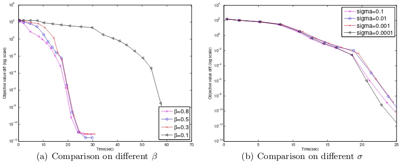
We adopt Armijo’s rule (Bertsekas, 1995; Tseng and Yun, 2007) and try step-sizes α∈ {β0, β1, β2, . . .} with a constant decrease rate 0 < β <1 (typicallyβ = 0.5), until we find the smallestk∈Nwithα=βksuch thatX+αD∗ is (a) positive-definite, and (b) satisfies the following sufficient decrease condition:
f(X+αD∗)≤f(X) +ασδ, δ= tr(∇g(X)TD∗) +kX+D∗k1,Λ− kXk1,Λ, (21)
where 0< σ <0.5. Notice that Condition (21) is a generalized version of Armijo line search rule for `1-regularized problems (see (Tseng and Yun, 2007; Yun and Toh, 2011) for the detail). We can verify positive definiteness while we compute the Cholesky factorization (costs O(p3) flops) needed for the objective function evaluation that requires the
compu-tation of log det(X+αD∗). The Cholesky factorization dominates the computational cost in the step-size computations. We use the standard convention in convex analysis that
f(X) = +∞ when X is not in the effective domain of f, i.e., X is not positive definite. Using this convention, (21) enforces positive definiteness of X+αD∗. Condition (21) has been proposed in Tseng and Yun (2007); Yun and Toh (2011) to ensure that the objective function value not only decreases but decreases by a certain amount ασδ, where δ mea-sures the closeness of the current solution to the global optimal. Our convergence proofs presented in Section 4 rely on this sufficient decrease condition.
In the rest of this section we present several lemmas about the step size computation. The reader mostly interested in the algorithm description may skip forward to Section 3.3 and revisit the details afterwards.
We start out by proving three important properties that we call (P1–P3) regarding the line search procedure governed by (21):
P1. The condition (21) is satisfied for some (sufficiently small) α, establishing that the algorithm does not enter into an infinite line search step. We note that in Proposition 3 below we show that the line search condition (21) can be satisfied for any symmetric matrixD (even one which is not the Newton direction).
P2. For the Newton direction D∗, the quantity δ in (21) is negative, which ensures that the objective function decreases. Moreover, to guarantee that Xt converges to the
global optimum, |δ| should be large enough when the current iterate Xt is far from
the optimal solution. In Proposition 4 we will prove the stronger condition that
δ≤ −(1/M2)kD∗k2
F for some constant M. kD∗k2F can be viewed as a measure of the
distance from optimality of the current iterate Xt, and this bound ensures that the
objective function decrease is proportional tokD∗k2
F.
P3. When X is close enough to the global optimum, the step size α = 1 will satisfy the line search condition (21). We will show this property in Proposition 5. Moreover, combined with the global convergence ofQUICproved in Theorem 12, this property
3.2.1 Detailed Proofs for P1-3
We first show the following useful property. For any matrices X, D, real number 0≤α ≤1 and Λ≥0 that generates the normk·k1,Λ, we have
kX+αDk1,Λ=kα(X+D) + (1−α)Xk1,Λ≤αkX+Dk1,Λ+ (1−α)kXk1,Λ. (22)
The above inequality can be proved by the convexity of k·k1,Λ, and will be used repeatedly
in this paper. Next we show an important property that all the iterates Xt will have
eigenvalues bounded away from zero. Since the updates in our algorithm satisfy the line search condition (21), andδ is always a negative number (see Proposition 4), the function value is always decreasing. It also follows that all the iterates {Xt}t=0,1,... belong to the
level set U defined by:
U ={X |f(X)≤f(X0) and X∈S++p }. (23)
Lemma 2 The level set U defined in (23) is contained in the set {X |mI X M I}
for some constants m, M > 0, if we assume that the off-diagonal elements of Λ and the diagonal elements of S are positive.
Proof We begin the proof by showing that the largest eigenvalue of anyX∈U is bounded by M, a constant that depends only on Λ, f(X0) and the matrix S. We note that S 0 and X0 implies tr(SX)≥0 and therefore:
f(X0)≥f(X)≥ −log detX+kXk1,Λ. (24)
SincekXk2 is the largest eigenvalue of thep×pmatrixX, we have log detX≤plog(kXk2).
Combine with (24) and the fact that the off-diagonal elements of Λ are no smaller than some
λ >0:
λX i6=j
|Xij|<kXk1,Λ ≤f(X0) +plog(kXk2). (25)
Similarly, kXk1,Λ≥0 implies that:
tr(SX)< f(X0) +plog(kXk2). (26)
Next, we introduce γ = miniSii and β = maxi6=j|Sij| and split tr(SX) into diagonal and
off-diagonal terms in order to bound it:
tr(SX) =X
i
SiiXii+
X
i6=j
SijXij ≥γtr(X)−β
X
i6=j
|Xij|.
Since kXk2 ≤tr(X),
γkXk2 ≤γtr(X)≤tr(SX) +β
X
i6=j
|Xij|.
Combine with (25) and (26) to get:
The left hand side of inequality (27), as a function of kXk2, grows much faster than the right hand side (note γ >0), and therefore kXk2 can be upper bounded by M, whereM
depends on the values of f(X0), S and Λ.
In order to prove the lower bound, we consider the smallest eigenvalue ofX denoted by
aand use the upper bound on the other eigenvalues to get:
f(X0)> f(X)>−log detX≥ −loga−(p−1) logM, (28)
which shows thatm=e−f(X0)M−(p−1) is a lower bound fora.
We note that the conclusion of the lemma also holds if the conditions on Λ and S are replaced by only the requirement that the diagonal elements of Λ are positive, see Banerjee et al. (2008). We emphasize that Lemma 2 allows the extension of the convergence results to the practically important case when the regularization does not penalize the diagonal, i.e., Λii = 0 ∀i. In subsequent arguments we will continue to refer to the minimum and
maximum eigenvaluesm and M established in Lemma 2.
Proposition 3 (corresponds to Property P1) For anyX0and symmetricD, there exists an α >¯ 0 such that for all α < α¯, the matrix X +αD satisfies the line search condition (21).
Proof When α < σn(X)/kDk2 (whereσn(X) stands for the smallest eigenvalue ofX and
kDk2 is the induced 2-norm of D, i.e., the largest eigenvalue in magnitude of D), we have kαDk2 < σn(X), which implies thatX+αD0. So we can write:
f(X+αD)−f(X) =g(X+αD)−g(X) +kX+αDk1,Λ− kXk1,Λ
≤g(X+αD)−g(X) +α(kX+Dk1,Λ− kXk1,Λ), by (22)
=αtr((∇g(X))TD) +O(α2) +α(kX+Dk1,Λ− kXk1,Λ)
=αδ+O(α2).
Therefore for any fixed 0 < σ < 1 and sufficiently small α, the line search condition (21) must hold.
Proposition 4 (corresponds to Property P2) δ =δJ(X) as defined in the line search
condition (21) satisfies
δ≤ −(1/kXk22)kD∗k2F ≤ −(1/M2)kD∗k2F, (29)
where M is as in Lemma 2.
Proof We first show thatδ =δJ(X) in the line search condition (21) satisfies
δ= tr((∇g(X))TD∗) +kX+D∗k1,Λ− kXk1,Λ≤ −vec(D∗)T∇2g(X) vec(D∗), (30)
According to the definition of D∗≡DJ∗(X) in (20), for all 0< α <1 we have:
tr(∇g(X)TD∗) +1 2vec(D
∗
)T∇2g(X) vec(D∗) +kX+D∗k1,Λ ≤
tr(∇g(X)TαD∗) +1
2vec(αD
∗)T∇2g(X) vec(αD∗) +kX+αD∗k
1,Λ. (31)
We combine (31) and 22 to yield:
tr(∇g(X)TD∗) +1 2vec(D
∗)T∇2g(X) vec(D∗) +kX+D∗k
1,Λ≤ αtr(∇g(X)TD∗) +1
2α
2vec(D∗)T∇2g(X) vec(D∗) +αkX+D∗k
1,Λ+ (1−α)kXk1,Λ.
Therefore
(1−α)[tr(∇g(X)TD∗) +kX+D∗k1,Λ− kXk1,Λ] +
1 2(1−α
2) vec(D∗)T∇2g(X) vec(D∗)≤0.
Divide both sides by 1−α >0 to get:
tr(∇g(X)TD∗) +kX+D∗k1,Λ− kXk1,Λ+
1
2(1 +α) vec(D
∗
)T∇2g(X) vec(D∗)≤0.
By taking the limit as α↑1, we get:
tr(∇g(X)TD∗) +kX+D∗k1,Λ− kXk1,Λ≤ −vec(D∗)T∇2g(X) vec(D∗),
which proves (30).
Since ∇2g(X) =X−1⊗X−1 is positive definite, (30) ensures that δ <0 for all X 0.
Since the updates in our algorithm satisfy the line search condition (21), we have established that the function value is decreasing. It also follows that all the iterates{Xt}t=0,1,... belong
to the level setU defined by (23). Since∇2g(X) =X−1⊗X−1, the smallest eigenvalue of
∇2g(X) is 1/kXk2
2, and we combine with Lemma 2 to get (29).
The eigenvalues of any iterate X are bounded by Lemma 2, and therefore ∇2g(X) = X−1⊗X−1 is Lipschitz continuous. Next, we prove that α = 1 satisfies the line search condition in a neighborhood of the global optimum X∗.
Proposition 5 (corresponds to Property P3) Assume that ∇2g is Lipschitz
continu-ous, i.e., ∃L >0 such that ∀t >0 and any symmetric matrix D,
k∇2g(X+tD)− ∇2g(X)kF ≤LktDkF =tLkDkF. (32)
Then, if X is close enough to X∗, the line search condition (21) will be satisfied with step size α= 1.
|˜g00(t)−g˜00(0)|:
|˜g00(t)−g˜00(0)| = |vec(D)T(∇2g(X+tD)− ∇2g(X)) vec(D)|
≤ kvec(D)T(∇2g(X+tD)− ∇2g(X))k2kvec(D)k2 (by Cauchy-Schwartz) ≤ kvec(D)k22k∇2g(X+tD)− ∇2g(X)k2 (by definition of k · k2 norm)
≤ kDk2Fk∇2g(X+tD)− ∇2g(X)kF (since k · k2 ≤ k · kF for any matrix)
≤ kDk2FtLkDkF by (32)
= tLkDk3
F.
Therefore, an upper bound for ˜g00(t):
˜
g00(t)≤˜g00(0) +tLkDk3
F = vec(D)T∇2g(X) vec(D) +tLkDk3F.
Integrate both sides to get
˜
g0(t)≤˜g0(0) +tvec(D)T∇2g(X) vec(D) +1 2t
2LkDk3
F
= tr((∇g(X))TD) +tvec(D)T∇2g(X) vec(D) +1 2t
2LkDk3
F.
Integrate both sides again:
˜
g(t)≤g˜(0) +ttr((∇g(X))TD) +1 2t
2vec(D)T∇2g(X) vec(D) +1
6t
3LkDk3
F.
Taking t= 1 we have
g(X+D)≤g(X) + tr(∇g(X)TD) +1
2vec(D)
T∇2g(X) vec(D) +1
6LkDk
3
F
f(X+D)≤g(X) +kXk1,Λ+ (tr(∇g(X)TD) +kX+Dk1,Λ− kXk1,Λ) + 1
2vec(D)
T∇2g(X) vec(D) +1
6LkDk
3
F
≤f(X) +δ+1
2vec(D)
T∇2g(X) vec(D) + 1
6LkDk
3
F
≤f(X) +δ 2 +
1 6LkDk
3
F by (30)
≤f(X) + (1 2 −
1 6LM
2kDk
F)δ (by Proposition 4)
≤f(X) +σδ (assuming Dis close to 0).
The last inequality holds if 1/2−LM2kDk
F/6> σwhich is guaranteed ifXis close enough
3.3 Identifying Which Variables to Update
In this section, we use the stationary condition of the Gaussian MLE problem to select a subset of variables to update in any Newton direction computation. Specifically, we partition the variables intofreeandfixedsets based on the value of the gradient at the start of the outer loop that computes the Newton direction. We define the free set Sf ree and
fixedset Sf ixed as:
Xij ∈Sf ixed if |∇ijg(X)| ≤λij, and Xij = 0,
Xij ∈Sf ree otherwise. (33)
We will now show that a Newton update restricted to the fixed set of variables would not change any of the coordinates in that set. In brief, the gradient condition|∇ijg(X)| ≤ λij
entails that the inner coordinate descent steps, according to the update in (16), would set these coordinates to zero, so they would not change since they were zero to begin with.
To derive the optimality condition, we begin by introducing the minimum-norm subgra-dient off and relate it to the optimal solution X∗ of (3).
Definition 6 The minimum-norm subgradient gradSijf(X) is defined as follows:
gradSijf(X) =
∇ijg(X) +λij if Xij >0,
∇ijg(X)−λij if Xij <0,
sign(∇ijg(X)) max(|∇ijg(X)| −λij,0) if Xij = 0.
Lemma 7 For any index set J, gradSijf(X) = 0 ∀(i, j) ∈ J if and only if ∆∗ = 0 is a solution of the following optimization problem:
arg min
∆ f(X+ ∆) such that ∆ij = 0 ∀(i, j)∈/J. (34)
Proof Any optimal solution ∆∗ for (34) must satisfy the following, for all (i, j)∈J,
∇ijg(X+ ∆∗)
=−λij ifXij + ∆∗ij >0,
=λij ifXij + ∆∗ij <0,
∈[−λij λij] ifXij + ∆∗ij = 0.
(35)
It can be seen immediately that ∆∗ = 0 satisfies (35) if and only if gradSijf(X) = 0 for all (i, j)∈J.
In our case, ∇g(X) =S−X−1 and therefore
gradSijf(X) =
(S−X−1)ij+λij ifXij >0,
(S−X−1)
ij−λij ifXij <0,
sign((S−X−1)ij) max(|(S−X−1)ij| −λij,0) ifXij = 0.
Therefore, takingJ =Sf ixed in Lemma 7, we can show that for anyXtand corresponding
fixed and free setsSf ixed andSf ree as defined by (33), ∆∗ = 0 is the solution of the following
optimization problem:
arg min
∆ f(Xt+ ∆) such that ∆ij = 0 ∀(i, j)∈Sf ree.
Based on the above property, if we perform block coordinate descent restricted to the fixed set, then no updates would occur. We then perform the coordinate descent updates restricted to only the free set to find the Newton direction. With this modification, the number of variables over which we perform the coordinate descent update (16) can be potentially reduced from p2 to the number of non-zeros in Xt. When the solution is sparse
(depending on the value of Λ) the number of free variables can be much smaller thanp2 and we can obtain huge computational gains as a result. In essence, we very efficiently select a subset of the coordinates that need to be updated.
The attractive facet of this modification is that it leverages sparsity of the solution and intermediate iterates in a manner that falls within the block coordinate descent framework of Tseng and Yun (2007). The index setsJ0, J1, . . . corresponding to the block coordinate
descent steps in the general setting of Tseng and Yun (2007)[p. 392] need to satisfy a Gauss-Seidel type of condition:
[
j=0,...,T−1
Jt+j ⊇ N ∀t= 1,2, . . . (36)
for some fixed T, where N denotes the full index set. In our framework J0, J2, . . . denote the fixed sets at various iterations, and J1, J3, . . . denote the free sets. Since J2i and J2i+1
is a partitioning of N the choice T = 3 will suffice. But will the size of the free set be small? We initialize X0 to a diagonal matrix, which is sparse. The following lemma shows that after a finite number of iterations, the iteratesXt will have a similar sparsity pattern
as the limitX∗. Lemma 8 is actually an immediate consequence of Lemma 14 in Section 4.
Lemma 8 Assume that {Xt} converges to X∗, the optimal solution of (3). If for some
index pair(i, j),|∇ijg(X∗)|< λij (so that Xij∗ = 0), then there exists a constantt >¯ 0 such
that for all t >¯t, the iterates Xt satisfy
|∇ijg(Xt)|< λij and (Xt)ij = 0. (37)
Note that |∇ijg(X∗)| < λij implies Xij∗ = 0 from the optimality condition of (3). This
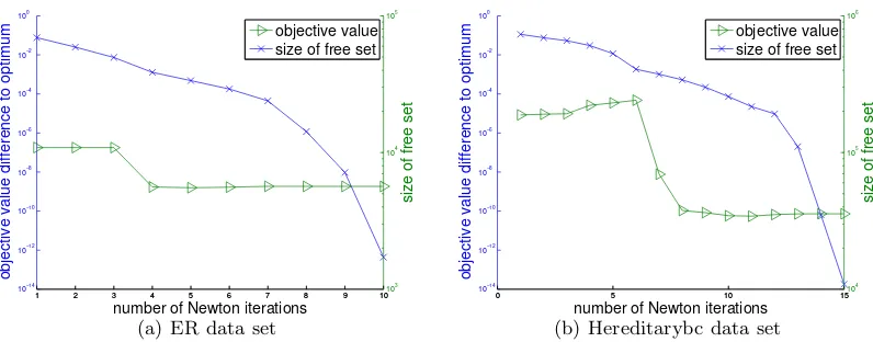
theorem shows that after ¯t-th iteration we can ignore all the indexes that satisfies (37), and in practice we can use (37) as a criterion for identifying the fixed set. A similar variable selection strategy is used in SVM (so called shrinking) and`1-regularized logistic regression problems as mentioned in Yuan et al. (2010). In our experiments, we demonstrate that this strategy reduces the size of the free set very quickly.
Lemma 8 suggests that QUIC can identify the zero pattern in finite steps. As we will
prove later,QUIChas an asymptotic quadratic convergence rate and therefore once the zero
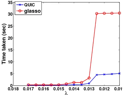
3.4 The Block-Diagonal Structure of X∗
It has been shown recently (Mazumder and Hastie, 2012; Witten et al., 2011) that when the thresholded covariance matrixE defined byEij =S(Sij, λ) = sign(Sij) max(|Sij| −λ,0)
has the following block-diagonal structure:
E=
E1 0 . . . 0 0 E2 . . . 0
..
. ... ... ...
0 0 0 Ek
, (38)
then the solution X∗ of the inverse covariance estimation problem (2) also has the same block-diagonal structure:
X∗ =
X1∗ 0 . . . 0 0 X2∗ . . . 0
..
. ... ... ...
0 0 0 Xk∗
.
This result can be extended to the case when the elements are penalized differently, i.e.,
λij’s are different. Then, if Eij = S(Sij, λij) is block diagonal, so is the solution X∗ of
(3), see Hsieh et al. (2012). Thus eachXi∗ can be computed independently. Based on this observation one can decompose the problem into sub-problems of smaller sizes, which can be solved much faster. In the following, we show that our updating rule and fixed/free set selection technique can automatically detect this block-diagonal structure for free.
Recall that we have a closed form solution in the first iteration when the input is a diagonal matrix. Based on (19), sinceXij = 0 for all i6=j in this step, we have
Dij =XiiXjjS(−Sij, λij) =−XiiXjjS(Sij, λij) for all i6=j.
We see that after the first iteration the nonzero pattern of X will be exactly the same as the nonzero pattern of the thresholded covariance matrix E as depicted in (38). In order to establish that the same is true at each subsequent step, we complete our argument using induction, by showing that the non-zero structure is preserved.
More precisely, we show that the off-diagonal blocks always belong to the fixed set if |Sij| ≤ λij. Recall the definition of the fixed set in (33). We need to check whether
|∇ijg(X)| ≤ λij for all (i, j) in the off-diagonal blocks of E, whenever X has the same
block-diagonal structure as E. Taking the inverse preserves the diagonal structure, and therefore ∇ijg(X) = Sij −Xij−1 =Sij for all such (i, j). We conclude noting that Eij = 0
implies that|∇ijg(X)| ≤λij, meaning that (i, j) will belong to thefixedset.
We decompose the matrix into smaller blocks prior to running Cholesky factorization to avoid the O(p3) time complexity on the whole problem. The connected components of
X can be detected in O(kXk0) time, which is very efficient when X is sparse. A detailed description ofQUIC is presented in Algorithm 2.
4. Convergence Analysis
In Section 3, we introduced the main ideas behind ourQUICalgorithm. In this section, we
Algorithm 2: QUadratic approximation for sparse Inverse Covariance estimation (QUIC)
Input : Empirical covariance matrixS (positive semi-definite p×p), regularization parameter matrix Λ, initialX00, parameters 0< σ <0.5, 0< β <1 Output: Sequence ofXt converging to arg minX0f(X), where
f(X) =g(X) +h(X), where g(X) =−log detX+ tr(SX), h(X) =kXk1,Λ.
1 Compute W0=X0−1. 2 for t= 0,1, . . . do
3 D= 0, U = 0
4 while not converged do
5 Partition the variables into fixed and free sets:
6 Sf ixed:={(i, j)| |∇ijg(Xt)| ≤λij and (Xt)ij = 0},
Sf ree:={(i, j)| |∇ijg(Xt)|> λij or (Xt)ij 6= 0}.
7 for (i, j)∈Sf ree do
8 a=wij2 +wiiwjj, b=sij−wij +wT·iu·j, c=xij +dij
9 µ=−c+S(c−b/a, λij/a)
10 dij ←dij +µ, ui·←ui·+µwj·, uj·←uj·+µwi·
11 end
12 end
13 forα= 1, β, β2, . . . do
14 Compute the Cholesky factorization LLT =Xt+αD.
15 if Xt+αD0 then
16 Compute f(Xt+αD) fromL andXt+αD
17 if f(Xt+αD)≤f(Xt) +ασ[tr(∇g(Xt)D) +kXt+Dk1,Λ− kXk1,Λ]then
18 break
19 end
20 end
21 end
22 Xt+1 =Xt+αD
23 Compute Wt+1=Xt−+11 reusing the Cholesky factor.
24 end
rate is quadratic. Banerjee et al. (2008) showed that for the special case where Λij = λ
the optimization problem (2) has a unique global optimum and that the eigenvalues of the primal optimal solution X∗ are bounded. In the following, we show this result for more general Λ where only the off-diagonal elements need to be positive.
Theorem 9 There exists a unique minimizer X∗ for the optimization problem (3), where
λij >0 for i6=j, andλij ≥0.
Since kXk1,Λ is convex and −log det(X) is strongly convex, we have thatf(X) is strongly convex on the compact setS, and therefore the minimizerX∗ is unique (Apostol, 1974).
4.1 Convergence Guarantee
In order to show thatQUICconverges to the optimal solution, we consider a more general
setting of the quadratic approximation algorithm: at each iteration, the iterateYtis updated
by Yt+1 = Yt+αtDJ∗t(Yt) where Jt is a subset of variables chosen to update at iteration t, DJ∗t(Yt) is the Newton direction restricted to Jt defined by (20), and αt is the step size
selected by the Armijo rule given in Section 3.2. The algorithm is summarized in Algorithm 3. Similar to the block coordinate descent framework of Tseng and Yun (2007), we assume the index set Jt satisfies a Gauss-Seidel type of condition:
[
j=0,...,T−1
Jt+j ⊇ N ∀t= 1,2, . . . . (39)
Algorithm 3: General Block Quadratic Approximation method for Sparse Inverse Covariance Estimation
Input : Empirical covariance matrixS (positive semi-definite p×p), regularization parameter matrix Λ, initialY0, inner stopping tolerance
Output: Sequence ofYt. 1 for t= 0,1, . . . do
2 Generate a variable subsetJt.
3 Compute the Newton direction Dt∗≡DJ∗
t(Yt) by (20).
4 Compute the step-size αt using theArmijo-rule based step-size selection in (21). 5 UpdateYt+1 =Yt+αtDt∗.
6 end
In QUIC, J0, J2, . . . denote the fixed sets and J1, J3, . . . denote the free sets. If
{Xt}t=0,1,2,... denotes the sequence generated by QUIC, then
Y0=Y1 =X0, Y2=Y3 =X1, . . . , Y2i=Y2i+1=Xi.
Moreover, since eachJ2i andJ2i+1 is a partitioning ofN, the choiceT = 3 will satisfy (39).
In the rest of this section, we show that{Yt}t=0,1,2,... converges to the global optimum, thus
{Xt}t=0,1,2,... generated byQUIC also converges to the global optimum.
Our first step towards the convergence proof is a lemma on convergent subsequences.
Lemma 10 For any convergent subsequence Yst → Y¯ where Y¯ is a limit point, we have D∗st ≡D∗J
st(Yst)→0.
We proceed to prove the statement by contradiction. If D∗st does not converge to 0, then there exists an infinite index set T ⊆ {s1, s2, . . .} and η > 0 such that kD∗tkF > η
for all t∈ T. According to Proposition 4, δst is bounded away from 0, therefore δst 6→ 0,
while αst → 0. We can assume without loss of generality that αst <1 ∀t, that is the line
search condition is not satisfied in the first attempt. We will work in this index set T in the derivations that follow.
The line search step sizeαt<1 (t∈ T) satisfies (21), butαt=αt/β does not satisfy (21)
by the minimality of our line search procedure. So we have:
f(Yt+αtDt∗)−f(Yt)> σαtδt. (40)
If Yt+αtDt∗ is not positive definite, then as is standard, f(Yt+αtD∗t) = ∞, so (40) still
holds. We expand (40) and apply 22 to get
σαtδt≤g(Yt+αtDt∗)−g(Yt) +kYt+αtD∗tk1,Λ− kYtk1,Λ
≤g(Yt+αtDt∗)−g(Yt) +αt(kYt+D∗tk1,Λ− kYtk1,Λ),∀t∈ T.
By the definition ofδt, we have:
σδt≤
g(Yt+αtDt∗)−g(Yt)
αt
+δt−tr(∇g(Yt)TD∗t),
(1−σ)(−δt)≤
g(Yt+αtD∗t)−g(Yt)
αt
−tr(∇g(Yt)TDt∗).
By Proposition 4 we haveδt≤ −(1/M2)kD∗tk2F, so usingkD ∗
tkto denotekD∗tkF for the rest
of the proof, we get
(1−σ)M−2kDt∗k2 ≤ g(Yt+αtD
∗
t)−g(Yt)
αt
−tr(∇g(Yt)TDt∗)
(1−σ)M−2kDt∗k ≤
gYt+αtkD∗tk D∗t
kD∗
tk
−g(Yt)
αtkD∗tk
−tr
∇g(Yt)T
Dt∗
kDt∗k
.
We set ˆαt=αtkD∗tk. SincekD∗tk> η for allt∈ T we have:
(1−σ)M−2η <
gYt+ ˆαt D ∗
t
kD∗
tk
−g(Yt)
ˆ
αt
−tr
∇g(Yt)T
Dt∗
kDt∗k
= ˆ
αttr
∇g(Yt) D ∗
t
kD∗
tk
+O( ˆα2t) ˆ
αt
−tr
∇g(Yt)T
Dt∗
kDt∗k
=O( ˆαt). (41)
Again, by Proposition 4,
−αtδt≥αtM−2kDt∗k2 > M−2αtkDt∗kη.
Since {αtδt}t → 0, it follows that {αtkD∗tk}t → 0 and{αˆt}t → 0. Taking limit of (41) as
t∈ T and t→ ∞, we have
a contradiction, finishing the proof.
Now that we have proved that DJ∗t converges to zero for the converging subsequence, we next show thatD∗J is closely related to the minimum-norm subgradient gradSf(Y) (see Definition 6), which in turn is an indicator of optimality as proved in Lemma 7.
Lemma 11 For any index setJ and positive definiteY,D∗J(Y) = 0if and only ifgradSijf(Y) = 0 for all (i, j)∈J.
Proof The optimality condition of (20) can be written as
∇ijg(X) + (∇2g(X) vec(D))ij
=−λ ifXij +Dij >0
=λ ifXij +Dij <0
∈[−λ, λ] ifXij +Dij = 0,
∀(i, j)∈J. (42)
D∗J(Y) = 0 if and only if D∗ = 0 satisfies (42), and this condition is equivalent to (35) restricted to (i, j)∈J, which in turn is equivalent to the optimality condition off. Therefore
D∗J(Y) = 0 iff gradSijf(Y) = 0 for all (i, j)∈J.
Based on these lemmas, we are now able to prove our main convergence theorem.
Theorem 12 Algorithm 3 converges to the unique global optimum Y∗.
Proof Since all the iterates Yt are in a compact set (as shown in Lemma 2), there exists
a subsequence{Yt}T that converges to a limit point ¯Y. Since the cardinality of each index
set Jt selected is finite, we can further assume that Jt = ¯J0 for all t ∈ T¯, where ¯T is a
subsequence ofT. From Lemma 10, D∗J¯0(Yt)→0. By continuity of ∇g(Y) and ∇2g(Y), it
is easy to show that DJ∗¯0(Yt) → DJ∗¯0( ¯Y). Therefore DJ∗¯0( ¯Y) = 0. Based on Lemma 11, we
have
gradSijf(Y) = 0 for all (i, j)∈J0.¯
Furthermore,{D∗J¯
0(Yt)}T →0 andkYt−Yt+1kF ≤ kD
∗
¯
J0(Yt)kF, so{Yt+1}t∈T also converges
to ¯Y. By considering a subsequence ofT if necessary, we can further assume thatJt+1 = ¯J1
for all t∈ T. By the same argument, we can show that{DJ∗
t+1(Yt)}T →0, soD
∗
¯
J1( ¯Y) = 0.
Similarly, we can show thatD∗J¯t( ¯Y) = 0∀t= 0, . . . , T−1 can be assumed for an appropriate
subset of T. With assumption (39) and Lemma 11 we have
gradSijf( ¯Y) = 0 ∀i, j. (43)
Using Lemma 7 with J as the set of all variables, we can show that (43) implies that ¯Y is the global optimum.
It is straightforward to generalize Theorem 12 to prove the convergence of block coordi-nate descent when the Hessian∇2g(X) is replaced by another positive definite matrix. The
4.2 Asymptotic Convergence Rate
Newton methods on constrained minimization problems:
The convergence rate of the Newton method on bounded constrained minimization has been studied in Levitin and Polyak (1966) and Dunn (1980). Here, we briefly mention their results.
Assume we want to solve a constrained minimization problem
min
x∈ΩF(x),
where Ω is a nonempty subset of Rn denoting the constraint set and F : Rn → R has a second derivative ∇2F(x). Then beginning from x
0, the natural Newton updates entail
computing the (k+ 1)-st iterate xk+1 as xk+1 = arg min
x∈Ω∇F(xk)
T(x−x
k) +
1
2(x−xk)
T∇2F(x
k)(x−xk). (44)
For simplicity, we assume that F is strictly convex, and has a unique minimizer x∗ in Ω. Then the following theorem holds.
Theorem 13 (Theorem 3.1 in Dunn, 1980) AssumeF is strictly convex, has a unique minimizer x∗ in Ω, and that ∇2F(x) is Lipschitz continuous. Then for all x
0 sufficiently
close to x∗, the sequence{xk} generated by (44)converges quadratically to x∗.
This theorem is proved in Dunn (1980). In our case, the objective function f(X) is non-smooth so Theorem 13 does not directly apply. Instead, we will first show that after a finite number of iterations the sign of the iterates {Xt} generated by QUICwill not change, so
that we can then use Theorem 13 to establish asymptotic quadratic convergence.
Quadratic convergence rate for QUIC:
Unlike as in (44), our Algorithm 3 does not perform an unrestricted Newton update: it iter-atively selects subsets of variables{Jt}t=1,...(fixedand freesets), and computes the Newton
direction restricted to the free sets. In the following, we show that the sequence{Xt}t=1,2,...
generated byQUICdoes ultimately converge quadratically to the global optimum.
Assume X∗ is the optimal solution, then we can divide the index set withλij 6= 0 into
three subsets:
P ={(i, j)|Xij∗ >0}, N ={(i, j)|Xij∗ <0}, Z ={(i, j)|Xij∗ = 0}. (45)
From the optimality condition forX∗,
∇ijg(X∗)
=−λij if (i, j)∈P,
=λij if (i, j)∈N,
∈[−λij, λij] if (i, j)∈Z.
(46)
Lemma 14 Assume that the sequence {Xt} converges to the global optimum X∗. Then
there exists a ¯t such that for all t >¯t,
(Xt)ij
≥0 if (i, j)∈P,
≤0 if (i, j)∈N,
= 0 if (i, j)∈Z.
Proof We prove the case for (i, j) ∈ P by contradiction, the other two cases can be handled similarly. If we cannot find a ¯t satisfying the first condition in (47), then there exists an infinite subsequence{Xat}such that for eachat there exists a (i, j)∈P such that
(Xat)ij <0. Since the cardinality ofP is finite, we can further find a specific pair (i, j)∈P
such that (Xst)ij <0 for all st, where st is a subsequence of at. We consider the update
fromXst−1 toXst. From Lemma 5, we can assume that st is large enough so that the step
size equals 1, thereforeXst =Xst−1+D
∗(X
st−1) whereD
∗(X
st−1) is defined in (20). Since
(Xst)ij = (Xst−1)ij+ (D
∗(X
st−1))ij <0, from the optimality condition of (20) we have
∇g(Xst−1) +∇ 2g(X
st−1) vec(D
∗(X
st−1))
ij =λij. (48)
SinceD∗(Xst−1) converges to 0, (48) implies that{∇ijg(Xst−1)}will converge toλij.
How-ever, (46) implies ∇ijg(X∗) =−λij, and by the continuity of ∇g we get that {∇ijg(Xt)}
converges to∇ijg(X∗) =−λij, a contradiction, finishing the proof.
The following lemma shows that the coordinates from the fixed set remain zero after a finite number of iterations.
Lemma 15 AssumeXt→X∗. There exists a¯t >0 such that variables in P orN will not
be selected to be in the fixed set Sf ixed, when t >¯t. That is,
Sf ixed ⊆Z.
Proof Since Xt converges to X∗, (Xt)ij converges to Xij∗ >0 if (i, j)∈P and toXij∗ <0
if (i, j) ∈N. Recall that (i, j) belongs to the fixed set only if (Xt)ij = 0. When t is large
enough, (Xt)ij 6= 0 when Xt ∈ P ∪N, therefore P and N will be disjoint from the fixed
set. Moreover, by the definition of the fixed set (33), indexes with λij = 0 will never be
selected. We proved that the fixed set will be a subset ofZ when tis large enough.
Theorem 16 The sequence{Xt}generated by theQUICalgorithm converges quadratically
to X∗, that is for some constant κ >0,
lim
t→∞
kXt+1−X∗kF
kXt−X∗k2F
=κ.
Proof First, if the index sets P, N and Z (related to the optimal solution) are given, the optimum of (2) is the same as the optimum of the following constrained minimization problem:
min
X −log det(X) + tr(SX) +
X
(i,j)∈P
λijXij−
X
(i,j)∈N
λijXij
s.t. Xij ≥0 ∀(i, j)∈P, Xij ≤0 ∀(i, j)∈N, Xij = 0 ∀(i, j)∈Z. (49)
In the following, we show that when t is large enough, QUIC solves the minimization
1. The constraints in (49) are satisfied by QUICiterates after a finite number of steps,
as shown in Lemma 14. Thus, the `1-regularized Gaussian MLE (3) is equivalent to the smooth constrained objective (49), since the constraints in (49) are satisfied when solving (3).
2. Since the optimization problem in (49) is smooth, it can be solved using constrained Newton updates as in (44). The QUIC update direction DJ∗(Xt) is restricted to a
set of free variables inJ. This is exactly equal to the unrestricted Newton update as in (44), after a finite number of steps, as established by Lemma 15. In particular, at each iteration the fixed set is contained in Z, which is the set which always satisfies (D∗t)Z= 0 for large enough t.
3. Moreover, by Lemma 5 the step size isα= 1 when tis large enough.
Therefore our algorithm is equivalent to the constrained Newton method in (44), which in turn converges quadratically to the optimal solution of (49). Since the revised prob-lem (49) and our original probprob-lem (3) has the same minimum, we have shown thatQUIC
converges quadratically to the optimum of (3).
Note that the constant κ is an increasing function of the Lipschitz constant of∇2g(X)
(as shown in Dunn, 1980), which is related to the quality of quadratic approximation. We have shown in Lemma 2 that mI X M I, therefore the Lipschitz constant of ∇2g(X) =X−1⊗X−1 is also upper bounded.
In the next section, we show that this asymptotic convergence behavior of QUIC is
corroborated empirically as well.
5. Experimental Results
We begin this section by comparing QUIC to other methods on synthetic and real data
sets. Then, we present some empirical analysis of QUICregarding the use of approximate
Newton directions and effects of parameterization.
5.1 Comparisons with Other Methods
We now compare the performance of QUICon both synthetic and real data sets to other
state-of-the-art methods. We have implemented QUICin C++ with MATLAB interface,
and all experiments were executed on 2.83GHz Xeon X5440 machines with 32G RAM and Linux OS.
We include the following algorithms in our comparisons:
• ALM: the Alternating Linearization Method proposed by Scheinberg et al. (2010). We use their MATLAB source code for the experiments.
• ADMM: another implementation of the alternating linearization method implemented by Boyd et al. (2012). The MATLAB code can be downloaded from http://www.
stanford.edu/~boyd/papers/admm/. We found that the default parameters (which
set the augmented Lagrangian parameter toρ= 50 and the over-relaxation parameter toα= 1.5. These parameters achieved the best speed on the ER data set.
• glasso: the block coordinate descent method proposed by Friedman et al. (2008).
We use the latest versionglasso1.7 downloaded fromhttp://www-stat.stanford.
edu/~tibs/glasso/. We directly call their Fortran procedure using a MATLAB
interface.
• PSM: the Projected Subgradient Method proposed by Duchi et al. (2008). We use the MATLAB source code provided in the PQN package (available at http://www.
cs.ubc.ca/~schmidtm/Software/PQN.html).
• SINCO: the greedy coordinate descent method proposed by Scheinberg and Rish
(2010). The code can be downloaded fromhttps://projects.coin-or.org/OptiML/
browser/trunk/sinco.
• IPM: An inexact interior point method proposed by Li and Toh (2010). The source code can be downloaded fromhttp://www.math.nus.edu.sg/~mattohkc/Covsel-0.
zip.
• PQN: the projected quasi-Newton method proposed by Schmidt et al. (2009). The source code can be downloaded fromhttp://www.di.ens.fr/~mschmidt/Software/
PQN.html.
In the following, we compareQUICand the above state-of-the-art methods on synthetic and real data sets with various settings of λ. Note that we use the identity matrix as the initial point forQUIC,ADMM,SINCO, andIPM. Since the identity matrix is not a dual
feasible point for dual methods (includingglasso,PSMand PQN), we use S+λI as the
dual initial point, which is the default setting in their original package.
5.1.1 Experiments on Synthetic Data Sets
We first compare the run times of the different methods on synthetic data. We generate the two following types of graph structures for the underlying Gaussian Markov Random Fields:
• Chain Graphs: The ground truth inverse covariance matrix Σ−1 is set to be Σ−1
i,i−1=
−0.5 and Σ−i,i1= 1.25.
• Graphs with Random Sparsity Structures: We use the procedure given in Example 1 in Li and Toh (2010) to generate inverse covariance matrices with random non-zero patterns. Specifically, we first generate a sparse matrix U with nonzero elements equal to ±1, set Σ−1 to be UTU and then add a diagonal term to ensure Σ−1 is
positive definite. We control the number of nonzeros in U so that the resulting Σ−1 has approximately 10p nonzero elements.
Data set Parameter Properties of the solution pattern p kΣ−1k
0 λ kX∗k0 TPR FPR
chain 1000 2998 0.4 3028 1 3×10⁻⁵
chain 4000 11998 0.4 11998 1 0
chain 10000 29998 0.4 29998 1 0
random
1000 10758 0.12 10414 0.69 4×10
−3
0.075 55830 0.86 0.05
random 4000 41112 0.08 41936 0.83 6×10
−3
0.05 234888 0.97 0.05
random 10000 91410 0.08 89652 0.90 4×10
−6
0.04 392786 1 3×10⁻³
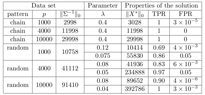
Table 1: The parameters and properties of the solution for the synthetic data sets. pstands for dimension, kΣ−1k
0 indicates the number of nonzeros in ground truth inverse
covariance matrix, kX∗k0 is the number of nonzeros in the solution. TPR and FPR denote the true and false recovery rates, respectively, defined in (50).
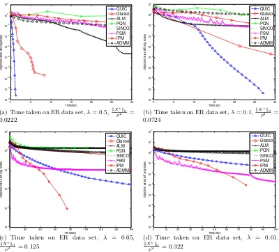
Table 1 shows the attributes of the synthetic data sets that we used in the timing comparisons. The dimensionality varies from {1000,4000,10000}. For chain graphs, we select λso that the solution has (approximately) the correct number of nonzero elements. In order to test the performance of the algorithms under different values of λ, for the case of random-structured graphs we considered two λvalues; one of which resulted in the discovery of the correct number of non-zeros and one which resulted in five-times thereof. We measured the accuracy of the graph structure recovered by the true positive rate (TPR) and false positive rate (FPR) defined as
TPR = |{(i, j)|(X
∗)
ij >0 andQij >0}|
|{(i, j)|Qij >0}|
,FPR = |{(i, j)|(X
∗)
ij >0 and Qij = 0}|
|{(i, j)|Qij = 0}|
,
(50)
whereQ is the ground truth sparse inverse covariance.
Since QUICdoes not natively compute a dual solution, the duality gap cannot be used as a stopping condition.2 In practice, we can use the minimum-norm sub-gradient (see Definition 6) as the stopping condition. There is no additional computational cost to this approach becauseX−1 is computed as part of the
QUICalgorithm. In the experiments, we
report the time for each algorithm to achieve-accurate solution defined byf(Xk)−f(X∗)< f(X∗). The global optimum X∗ is computed by running QUIC until it converges to a
solution withkgradSf(Xt)k<10−13.
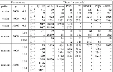
Table 2 shows the results for = 10−2 and 10−6, where= 10−2 tests the ability of the
algorithm to get a good initial guess (the nonzero structure), and= 10−6 tests whether the algorithm can achieve an accurate solution. Table 2 shows that QUICis consistently and
2. Note thatW =X−1 cannot be expected to satisfy the dual constraints|Wij−Sij| ≤λij. One could
projectX−1in order to enforce the constraints and use the resulting matrix to compute the duality gap.
0 5 10 15 20 25 30 35 40 10−14 10−12 10−10 10−8 10−6 10−4 10−2 10 Time(sec)
Objective value diff (log scale)
ALM PQN SINCO PSM IPM ADMM
(a) Objective value versus time on
chain1000
0 5 10 15 20 25 30 35 40
10−16 10−14 10−12 10−10 10−8 10−6 10−4 10−2 Time(sec)
Objective value diff (log scale)
ALM PQN SINCO PSM IPM ADMM
(b) Objective value versus time on ran-dom1000
0 5 10 15 20 25 30 35 40
0 0.1 0.2 0.3 0.4 0.5 0.6 0.7 0.8 0.9 1 Time(sec)
True positive rate
QUIC Glasso ALM PQN SINCO PSM IPM ADMM
(c) True positive rate versus time on chain1000
0 5 10 15 20 25 30 35 40
0 0.1 0.2 0.3 0.4 0.5 0.6 0.7 Time(sec)
True positive rate
QUIC Glasso ALM PQN SINCO PSM IPM ADMM
(d) True positive rate versus time on ran-dom1000
0 5 10 15 20 25 30 35 40
0 0.1 0.2 0.3 0.4 0.5 0.6 0.7 0.8 0.9 1 Time(sec)
False positive rate
QUIC Glasso ALM PQN SINCO PSM IPM ADMM
(e) False positive rate versus time on chain1000
0 5 10 15 20 25 30 35 40
0 0.1 0.2 0.3 0.4 0.5 0.6 0.7 0.8 0.9 1 Time(sec)
False positive rate
QUIC Glasso ALM PQN SINCO PSM IPM ADMM
(f) False positive rate versus time on ran-dom1000
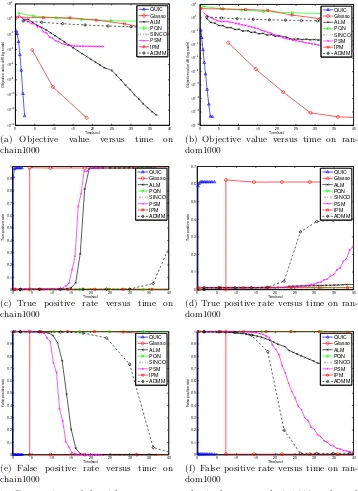
Figure 1: Comparison of algorithms on two synthetic data sets: chain1000 and random1000. The regularization parameterλis chosen to recover (approximately) correct num-ber of nonzero elements (see Table 1). We can see thatQUICachieves a solution
with better objective function value as well as better true positive and false pos-itive rates in both data sets. Notice that each marker in the figures indicates one iteration. Note that all results are averaged over 5 replicated runs.