An Investigation of Missing Data Methods for Classification Trees
Applied to Binary Response Data
Yufeng Ding [email protected]
Moody’s Investors Service 250 Greenwich Street New York, NY 10007
Jeffrey S. Simonoff [email protected]
New York University, Stern School of Business 44 West 4th Street
New York, NY 10012
Editor: Charles Elkan
Abstract
There are many different methods used by classification tree algorithms when missing data occur in the predictors, but few studies have been done comparing their appropriateness and performance. This paper provides both analytic and Monte Carlo evidence regarding the effectiveness of six popular missing data methods for classification trees applied to binary response data. We show that in the context of classification trees, the relationship between the missingness and the dependent variable, as well as the existence or non-existence of missing values in the testing data, are the most helpful criteria to distinguish different missing data methods. In particular, separate class is clearly the best method to use when the testing set has missing values and the missingness is related to the response variable. A real data set related to modeling bankruptcy of a firm is then analyzed. The paper concludes with discussion of adaptation of these results to logistic regression, and other potential generalizations.
Keywords: classification tree, missing data, separate class, RPART, C4.5, CART
1. Classification Trees and the Problem of Missing Data
Like most statistics or machine learning methods, “base form” classification trees are designed assuming that data are complete. That is, all of the values in the data matrix, with the rows being the observations (instances) and the columns being the variables (attributes), are observed. However, missing data (meaning that some of the values in the data matrix are not observed) is a very common problem, and for this reason classification trees have to, and do, have ways of dealing with missing data in the predictors. (In supervised learning, an observation with missing response value has no information about the underlying relationship, and must be omitted. There is, however, research in the field of semi-supervised learning methods that tries to handle the situation where the response value is missing, for example, Wang and Shen 2007.)
Although there are many different ways of dealing with missing data in classification trees, there are relatively few studies in the literature about the appropriateness and performance of these missing data methods. Moreover, most of these studies limited their coverage to the simplest miss-ing data scenario, namely, missmiss-ing completely at random (MCAR), while our study shows that the missing data generating process is one of the two crucial criteria in determining the best missing data method. The other crucial criterion is whether or not the testing set is complete. The following two subsections describe in more detail these two criteria.
1.1 Different Types of Missing Data Generating Process
Data originate according to the data generating process (DGP) under which the data matrix is “gen-erated” according to the probabilistic relationships between the variables. We can think of the missingness itself as a random variable, realized as the matrix of the missingness indicator Im. Imis
generated according to the missingness generating process (MGP), which governs the relationship between Im and the variables in the data matrix. Im has the same dimension as the original data
matrix, with each entry equal to 0 if the corresponding original data value is observed and 1 if the corresponding original data value is not observed (missing). Note that an Imvalue not only can be
related to its corresponding original data value, but can also be related to other variables of the same observation.
Depending on the relationship between Imand the original data, Rubin (1976) and Little and
Ru-bin (2002) categorize the missingness into three different types. If Imis dependent upon the missing
Missingness is related to Missing Observed Response
values Predictors Variable LR Three-Letter
1 No No No MCAR − − −
2 No Yes No MAR −X−
3 Yes No No NMAR M− −
4 Yes Yes No NMAR M X−
5 No No Yes MAR − −Y
6 No Yes Yes MAR −X Y
7 Yes No Yes NMAR M−Y
8 Yes Yes Yes NMAR M X Y
Table 1: Eight missingness patterns investigated in this study and their correspondence to the cate-gorization MCAR, MAR and NMAR defined by Rubin (1976) and Little and Rubin (2002) (the LR column). The column Three-Letter shows the notation that is used in this paper.
In this paper, we investigate eight different missingness patterns, depending on the relationship between the missingness and three types of variables, the observed predictors, the unobserved pre-dictors (the missing values) and the response variable. The relationship is conditional upon other factors, for example, missingness is not dependent upon the missing values means that the miss-ingness is conditionally independent of the missing values given the observed predictors and/or the response variable. Table 1 shows their correspondence with the MCAR/MAR/NMAR catego-rization as well as the three-letter notation we use in this paper. The three letters indicate if the missingness is conditionally dependent on the missing values (M), on other predictors (X) and on the response variable (Y), respectively. As will be shown, the dependence of the missingness on the response variable (the letter Y) is the one that affects the choice of best missingness data method. Later in the paper, some derived notations are also used. For example, ∗X∗means the union of −X−,−XY, MX−and MXY, that is, the missingness is dependent upon the observed predictors, and it may or may not be related to the missing values and/or the response variable.
1.2 Scenarios Where the Testing Data May or May Not Be Complete
There are essentially two stages of applying classification trees, the training phase where the his-torical data (training set) are used to construct the tree, and the testing phase where the tree is put into use and applied to testing data. Similar to most other studies, this study deals with the scenario where missing data occur in the training set, but the testing set may or may not have missing values. One basic assumption is, of course, that the DGP (as well as MGP if the testing set also contains missing values) is the same for both the training set and the testing set.
to predict bankruptcy from ratios from one’s own company, it would be expected that all of the necessary information for prediction would be available, and thus the test set would be complete.
This study shows that when the missingness is dependent upon the response variable and the test set has missing values, separate class is the best missing data method to use. In other situations, the choice is not as clear, but some insights on effective choices are provided. The rest of paper provides detailed theoretical and empirical analysis and is organized as follows. Section 2 gives a brief introduction to the previous research on this topic. This is followed by discussion of the design of this study and findings in Section 3. The generality of the results are then tested on real data sets in Section 4. A brief extension of the results to logistic regression is presented in Section 5. We conclude with discussion of these results and future work in Section 6.
2. Previous Research
There have been several studies of missing data and classification trees in the literature. Liu, White, Thompson, and Bramer (1997) gave a general description of the problem, but did not discuss solu-tions. Saar-Tsechansky and Provost (2007) discussed various missing data methods in classification trees and proposed a cost-sensitive approach to the missing data problem for the scenario when miss-ing data occur only at the testmiss-ing phase, which is different from the problem studied here (where missing values occur in the training phase).
Kim and Yates (2003) conducted a simulation study of seven popular missing value methods but did not find any dominant method. Feelders (1999) compared the performance of surrogate split and imputation and found the imputation methods to work better. (These methods, and the methods described below, are described more fully in the next section.) Batista and Monard (2003) compared four different missing data methods, and found that 10 nearest neighbor imputation outperformed other methods in most cases. In the context of cost sensitive classification trees, Zhang, Qin, Ling, and Sheng (2005) studied four different missing data methods based on their performances on five data sets with artificially generated random missing values. They concluded that the internal node method (the decision rules for the observations with the next split variable missing will be made at the (internal) node) is better than the other three methods examined. Fujikawa and Ho (2002) compared several imputation methods based on preliminary clustering algorithms to probabilistic split on simulations based on several real data sets and found comparable performance. A weakness of all of the above studies is that they focused only on the restrictive MCAR situation.
Other studies examined both MAR and NMAR missingness. Kalousis and Hilario (2000) used simulations from real data sets to examine the properties of seven algorithms: two rule inducers, a nearest neighbor method, two decision tree inducers, a naive Bayes inducer, and linear discriminant analysis. They found that the naive Bayes method was by far most resilient to missing data, in the sense that its properties changed the least when the missing rate was increased (note that this resilience is related to, but not the same as, its overall predictive performance). They also found that the deleterious effects of missing data are more serious if a given amount of missing values are spread over several variables, rather than concentrated in a few.
dependence of missingness on the response variable was not examined. Multiple imputation was found to be most effective, with probabilistic split also performing reasonably well, although little difference was found between methods when the proportion of missing values was low. As would be expected, MCAR missingness caused the least problems for methods, while NMAR missingness caused the most, and as was also found by Kalousis and Hilario (2000), missingness spread over several predictors is more serious than if it is concentrated in only one. Twala, Jones, and Hand (2008) proposed a method closely related to creating a separate class for missing values, and found that its performance was competitive with that of likelihood-based multiple imputation.
The study described in the next section extends these previous studies in several ways. First, theoretical analyses are provided for simple situations that help explain observed empirical perfor-mance. We then extend these analyses to more complex situations and data sets (including large ones) using Monte Carlo simulations based on generated and real data sets. The importance of whether missing is dependent on the response variable, which has been ignored in previous studies on classification trees yet turns out to be of crucial importance, is a fundamental aspect of these results. The generality of the conclusions is finally tested using real data sets and application to logistic regression.
3. The Effectiveness of Missing Data Methods
The recursive nature of classification trees makes them almost impossible to analyze analytically in the general case beyond 2×2 tables (where there is only one binary predictor and a binary response variable). On the other hand, trees built on 2×2 tables, which can be thought of as “stumps” with a binary split, can be considered as degenerate classification trees, with a classification tree being built (recursively) as a hierarchy of these degenerate trees. Therefore, analyzing 2×2 tables can result in important insights for more general cases. We then build on the 2×2 analyses using Monte Carlo simulation, where factors that might have impact on performance are incrementally added, in order to see the effect of each factor. The factors include variation in both the data generating process (DGP) and the missing data generating process (MGP), the number and type of predictors in the data, the number of predictors that contain missing values, and the number of observations with missing data.
This study examines six different missing data methods: probabilistic split, complete case method, grand mode/mean imputation, separate class, surrogate split, and complete variable method. Probabilistic split is the default method ofC4.5 (Quinlan, 1993). In the training phase, observations with values observed on the split variable are split first. The ones with missing values are then put into each of the child nodes with a weight given as the proportion of non-missing instances in the child. In the testing phase, an observation with a missing value on a split variable will be associated with all of the children using probabilities, which are the weights recorded in the training phase. The complete case method deletes all observations that contain missing values in any of the predic-tors in the training phase. If the testing set also contains missing values, the complete case method is not applicable and thus some other method has to be used. In the simulations, we use C4.5 to
(category) of the predictor. This is trivial to apply when the original variable is categorical, where we can create a new category called “missing”. To apply the separate class method to a numerical variable, we give all of the missing values a single extremely large value that is obviously outside of the original data range. This creates the needed separation between the nonmissing values and the missing values, implying that any split that involves the variable with missing values will put all of the missing observations into the same branch of the tree. Surrogate split is the default method of
CART(realized usingRPART in this study; Breiman et al. 1998 and Therneau and Atkinson 1997).
It finds and uses a surrogate variable (or several surrogates in order) within a node if the variable for the next split contains missing values. In the testing phase, if a split variable contains missing values, the surrogate variables in the training phase are used instead. The complete variable method simply deletes all variables that contain missing values.
Before we start presenting results, we define a performance measure that is appropriate for mea-suring the impact of missing data. Accuracy, calculated as the percentage of correctly classified observations, is often used to measure the performance of classification trees. Since it can be af-fected by both the data structure (some data are intrinsically easier to classify than others) and by the missing data, this is not necessarily a good summary of the impact of missing data. In this study, we define a measure called relative accuracy (RelAcc), calculated as
RelAcc= Accuracy with missing data
Accuracy with original full data.
This can be thought of as a standardized accuracy, as RelAcc measures the accuracy achievable with missing values relative to that achievable with the original full data.
3.1 Analytical Results
In the following consistency theorems, the data are assumed to reflect the DGP exactly, and therefore the training set and the testing set are exactly the same. Several of the theorems are for 2×2 tables, and in those cases stopping and pruning rules are not relevant, since the only question is whether or not the one possible split is made. The proofs are thus dependent on the underlying parameters of the DGP and MGP, rather than on data randomly generated from them. It is important to recognize that these results are only designed to be illustrative of the results found in the much more realistic simulation analyses to follow. Proofs of all of the results are given in the appendix.
Before presenting the theorems, we define some terms to avoid possible confusion. First, a partition of the data refers to the grouping of the observations defined by the classification tree’s splitting rules. Note that it is possible for two different trees on the same data set to define the same partition. For example, suppose that there are only two binary explanatory variables, X1and X2, and
one tree splits on X1 then X2 while another tree splits on X2 then X1. In this case, these two trees
have different structures, but they can lead to the same partition of the data. Secondly, the set of rules defined by a classification tree consists of the rules defined by the tree leaves on each of the groups (the partition) of the data.
3.1.1 WHEN THETESTSET ISFULLYOBSERVEDWITHNOMISSINGVALUES
Theorem 1 Complete Case Method: If the MGP is conditionally independent of Y given X , then the tree built on the data containing missing values using the complete case method gives the same set of rules as the tree built on the original full data set.
Theorem 2 Complete Case Method: If the partition of the data defined by the tree built on the incomplete data is not changed from the one defined by the tree built on the original full data, the
loss in accuracy when the testing set is complete is bounded above by PM, where PMis the missing
rate, defined as the percentage of observations that contain missing values.
Theorem 3 Complete Case Method: If the partition of the data defined by the tree built on the incomplete data is not changed from the one defined by the tree built on the original full data, the relative accuracy when the testing set is complete is bounded below by
RelAccmin=
1−PM
1+PM ,
where PM is the missing rate. Notice that the tree structure itself could change as long as it gives
the same final partition of the data.
There are similar results in regression analyses as in Theorem 1. In regression analyses, when the missingness is independent of the response variable, by using only the complete observations, the parameter estimators are all unbiased (Allison, 2001). This implies that in theory, when the missingness is independent of the response variable, using complete cases only is not a bad approach on average. However, in practice, as will be seen later, deleting observations with missing values can cause severe loss in information, and thus has generally poor performance.
Theorem 4 Probabilistic Split: In a 2×2 data table, if the MGP is independent of either Y or X , given the other variable, then the following results hold for probabilistic split.
1. If X is not informative in terms of classification, that is, the majority classes of Y for different X values are the same, then probabilistic split will give the same rule as the one that would be obtained from the original full data;
2. If probabilistic split shows that X is informative in terms of classification, that is, the majority classes of Y for different X values are different, then it finds the same rule as the one that would be obtained from the original full data;
3. The absolute accuracy when the testing set is complete is bounded below by 0.5. Since the original full data accuracy is at most 1, the relative accuracy is also bounded below by 0.5.
Theorem 5 Mode Imputation: If the MGP is independent of Y , given X , then the same results hold for mode imputation as for probabilistic split under the conditions of Theorem 4.
Moreover, with 2×2 tables, the complete variable method will always have a higher than 0.5 accuracy since by ignoring the only predictor, we will always classify all of the data to the overall majority class and achieve at least 0.5 accuracy, and thus at least 0.5 relative accuracy. Together with Theorems 4 and 5, as well as the evidence to be shown in Figure 1, this is an indication that classification trees tend not to be hurt much by missing values, since trees built on 2×2 tables can be considered as degenerate classification trees and more complex trees are composites of these degenerate trees. The performance of a classification tree is the average (weighted by the number of observations at each leaf) over the degenerate trees at the leaf level, and, as will be seen later in the simulations, can often be quite good.
Surrogate split is not applicable to 2×2 tables because there are no other predictors. For 2×2 table problems with a complete testing set, separate class is essentially the same as the complete case method, because as long as the data are split according to the predictor (and it is very likely that this will be so), the separate class method builds separate rules for the observations with missing values; when the testing set is complete, the rules that are used in the testing phase are exactly the ones built on the complete observations. When there is more than one predictor, however, the creation of the “separate class” will save the observations with missing values from being deleted and affect the tree building process. It will very likely lead to a change in the tree structure. This, as will be seen, tends to have a favorable impact on the performance accuracy.
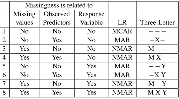
Figure 1 illustrates the lower bound calculated in Theorem 3. The illustration is achieved by Monte Carlo simulation of 2×2 tables. A 2×2 table with missing values has only eight cells, that is, eight different value combinations of the binary variables X , Y and M, where M is the missingness indicator such that M=0 if X is observed and M=1 if X is missing. There is one constraint, that the sum of the eight cell probabilities must equal one. Therefore, this table is determined by seven parameters. In the simulation, for each 2×2 table, the following seven parameters (probabilities) are randomly and independently generated from a uniform distribution between(0,1): (1)P(X=1),
(2)P(Y =1|X =0), (3)P(Y =1|X =1), (4)P(M=1|X =0,Y =0), (5)P(M=1|X =0,Y =1), (6)P(M=1|X =1,Y =0)and (7)P(M=1|X =1,Y =1). Here we assume the data tables reflect the true underlying DGP and MGP without random variation, and thus the expected performance of the classification trees can be derived using the parameters. In this simulation, sets of the seven parameters are generated (but no data sets are generated using these parameters) repeatedly, and the relative accuracy of each missing data method on each parameter set is determined. One million sets of parameters are generated for each missingness pattern.
Figure 1: Scatter plot and the corresponding quantile plot of the complete testing set RelAcc vs. missing rate of the complete case method when the MGP is dependent on the response variable. Recall that “∗ ∗Y” means the MGP is conditionally dependent on the response variable but no restriction on the relationship between the MGP and other variables, miss-ing or observed, is assumed. Each point in the scatter plot represents the result on one of the simulated data tables.
of data from the left to the right. Due to space limitations, we do not show quantile plots of other missing data methods and/or under different scenarios, but in all of the other plots, the quantile lines are all higher (that is, the quantile plot in Figure 1 shows the worst case scenario). The plots show that the missing data problem, when the missing rate is not too high, may not be as serious as we might have thought. For example, when 40% of the observations contain missing data, 80% of the time the expected relative accuracy is higher than 90%, and 90% of the time the expected relative accuracy is higher than 80%.
3.1.2 WHEN THETESTSETHASMISSINGVALUES
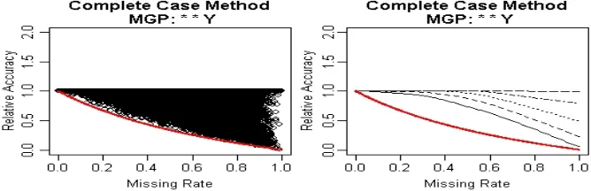
Theorem 6 Separate Class: In 2×2 data tables, if missing values occur in both the training set and the testing set, then the separate class method achieves the best possible performance.
Figure 2: Scatter plot of the separate class method with incomplete testing set. Each point in the scatter plot represents the result on one of the simulated data tables.
supporting evidence. Theorem 6 makes a fairly strong statement in the simple situation, and it will be seen to be strongly indicative of the results in more general cases.
3.2 Monte Carlo Simulations of General Data Sets
In this section extensions of the simulations in the last section are summarized.
3.2.1 ANOVERVIEW OF THESIMULATION
The following simulations are carried out.
1. 2×2 tables, missing values occur in the only predictor.
2. Up to seven binary predictors, missing values occur in only one predictor.
3. Eight binary predictors, missing values occur in two of them.
4. Twelve binary predictors, missing values occur in six of them.
5. Eight continuous predictors, missing values occur in two of them.
6. Twelve continuous predictors, missing values occur in six of them.
Two different scenarios of each of the last four simulations listed above were performed. In the first scenario, the six complete predictors are all independent of the missing ones, while in the second scenario three of the six complete predictors are related to the missing ones. Therefore, ten simulations were done in total.
In−sample accuracy
In−sample accuracy
Density
0.6 0.7 0.8 0.9 1.0
0.0
1.0
2.0
3.0
Out−of−sample accuracy
Out−of−sample accuracy
Density
0.5 0.6 0.7 0.8 0.9 1.0
0.0
1.0
2.0
3.0
In−sample AUC
In−sample AUC
Density
0.5 0.6 0.7 0.8 0.9 1.0
0
1
2
3
4
Out−of−sample AUC
Out−of−sample AUC
Density
0.5 0.6 0.7 0.8 0.9
0
4
8
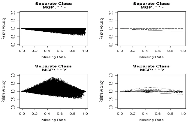
Figure 3: A summary of the tree performance on the simulated original full data.
each DGP, eight different MGPs are simulated to cover different types of missingness patterns. For each data set, the variables are generated sequentially in the order of the predictors, the response and the missingness. The probabilities associated with the binary response variable and the binary missingness variable are generated using conditional logit functions. The predictors may or may not be correlated with each other. Details about the simulations implementation can be found in Ding and Simonoff (2008). For each set of DGP/MGP, several different sample sizes are simulated to see any possible learning curve effect, since it was shown by Perlich, Provost, and Simonoff (2003) that sample size is an important factor in the effectiveness of classification trees. Figure 3 shows the distribution of the tree performance on the simulated original full data, as measured by accuracy and area under the ROC curve (AUC). As we can see, there is broad coverage of the entire range of strength of the underlying relationship. Also, as expected, the out-of-sample performance (on the test set) is generally worse than the in-sample performance (on the training set). When the in-sample AUC is close to 0.5, a tree is likely to not split and as a result, any missing data method will not actually be applied, resulting in equivalent performance over all of them. To make the comparisons more meaningful, we exclude the cases where the in-sample AUC is below 0.7. Lower thresholds for exclusion (0.55 and 0.6) yield very similar results.
Of the six missing data methods covered by this study, five of them, namely, complete case method, probabilistic split, separate class, imputation and complete variable method, are realized using C4.5. These methods are always comparable. However, surrogate split is carried out using
RPART, which makes it less comparable to the other methods because of differences betweenRPART
andC4.5 other than the missing data methods. To remedy this problem, we tuned theRPART
param-eters (primarily the parameter “cp”) so that it gives balanced results compared toC4.5 when applied to the original full data (i.e., each has a similar probability of outperforming the other), and special attention is given when comparingRPARTwith other methods. The out-of-sample performances of
P
P P
100 500 2000 10000
0 20 40 60 80 − − − Sample size
Winning pct of each method
C
C
C
S S S
M M M T T T D D D P P P
100 500 2000 10000
0
20
40
60
80
− − Y
Sample size
Winning pct of each method
C
C
C
S S S
M M M
T T T D D D P P P
100 500 2000 10000
0
20
40
60
80
− X −
Sample size
Winning pct of each method
C C C S S S M M M T T T D D D P P P
100 500 2000 10000
0
20
40
60
80
− X Y
Sample size
Winning pct of each method
C
C
C
S S S
M M M
T T T D D D P P P
100 500 2000 10000
0
20
40
60
80
M − −
Sample size
Winning pct of each method
C
C
C
S S S
MT MT M
T D D D P P P
100 500 2000 10000
0
20
40
60
80
M − Y
Sample size
Winning pct of each method
C
C
C
S S S
M M M
T T T D D D P P P
100 500 2000 10000
0
20
40
60
80
M X −
Sample size
Winning pct of each method
C
C
C
S S S
MT MT M
T D D D P P P
100 500 2000 10000
0
20
40
60
80
M X Y
Sample size
Winning pct of each method
C
C
C
S S S
M M M
T
T
T
D D
D
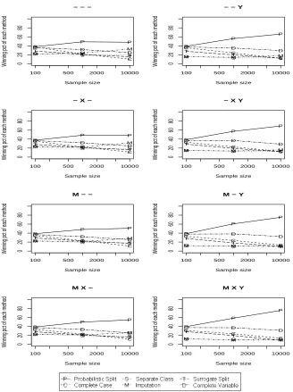
Figure 4: A summary of the order of six missing data methods when tested on a new complete testing set. The Y axis is the percentage of times each method is the best (including being tied with other methods; therefore the percentages do not sum up to one).
3.2.2 THETWO FACTORS THATDETERMINE THEPERFORMANCE OFDIFFERENTMISSING
DATAMETHODS
P
P
P
100 500 2000 10000
0 20 40 60 80 − − − Sample size
Winning pct of each method
C
C
C
S S S
M M M T T T D D
D P P P
100 500 2000 10000
0
20
40
60
80
− − Y
Sample size
Winning pct of each method
C
C
C
S S
S
MT MT M
T
D D
D
P P P
100 500 2000 10000
0
20
40
60
80
− X −
Sample size
Winning pct of each method
C
C
C S
S S
M M M
T
T
T D
D
D P P
P
100 500 2000 10000
0
20
40
60
80
− X Y
Sample size
Winning pct of each method
C
C
C
S S
S
MTD MDT MDT
P P P
100 500 2000 10000
0
20
40
60
80
M − −
Sample size
Winning pct of each method
C
C
C
S S S
M M M
T
T
T D
D
D P P
P
100 500 2000 10000
0
20
40
60
80
M − Y
Sample size
Winning pct of each method
C C C S S S
M M M
T
T T
D D
D
P P P
100 500 2000 10000
0
20
40
60
80
M X −
Sample size
Winning pct of each method
C
C
C
S S S
M M M
T
T T
D
D
D P P
P
100 500 2000 10000
0
20
40
60
80
M X Y
Sample size
Winning pct of each method
C C C S S S M M M T T T D D D
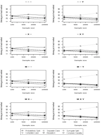
Figure 5: A summary of the order of six missing data methods when tested on a new incomplete testing set. The Y axis is the percentage of times each method is the best (including being tied with other methods).
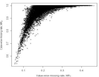
Figure 6: Plot of the case-wise missing rate MR2 versus the value-wise missing rate MR1 in the
simulations using the 36 real data sets.
Comparison of the right columns of Figures 4 and 5 shows that whether or not there are missing values in the testing set is the second important criterion in differentiating between the methods. The separate class method is strongly dominant when the testing set contains missing values and the missingness is related to the response variable. The reason for this is that when missing data exist in both the training phase and the testing phase, they become part of the data and the MGP becomes an essential part of the DGP. This, of course, requires the assumption that the MGP (as well as the DGP) is the same in both the training phase and the testing phase. Under this scenario, if the missingness is related to the response variable, then there is information about the response variable in the missingness, which should be helpful when making predictions. Separate class, by taking the missingness directly as an “observed” variable, uses the information in the missingness about the response variable most effectively and thus is the best method to use. As a matter of fact, as can be seen in the bottom rows of Figures 7 and 8 (which give average relative accuracies separated by missing rate), the average relative accuracy of separate class under this situation is larger than one, indicating, on average, a better performance than with the original full data.
On the other hand, when the missing data only occur in the training phase and the testing set does not have missing values, or when the missingness is not related to and carries no information about the response variable, the existence of missing values is a nuisance. Its only effect is to obscure the underlying DGP and thus would most likely reduce a tree’s performance. In this case, simulations show probabilistic split to be the dominantly best method. However, we don’t see this dominance later in results based on real data sets. More discussion of this point will follow in Section 4.
3.2.3 MISSINGRATEEFFECT
There are two ways of defining the missing rate: the percentage of predictor values that are missing from the data set (the value-wise missing rate, termed here MR1), and the percentage of observations
that contain missing values (the case-wise missing rate, termed here MR2). If there is only one
P P
P
100 500 2000 10000
0 20 40 60 80 100
Winning Pct / MGP: MXY / MR1<0.15
Sample size
Winning pct of each method C
C C S S S M M M T T T D D D P P P
100 500 2000 10000
0 20 40 60 80 100
Winning Pct / MGP: MXY / 0.2<MR1<0.3
Sample size
Winning pct of each method C
C C S S S M M M T T T D D D P P P 100 500 2000 10000
0 20 40 60 80 100
Winning pct / MGP: MXY / MR1>0.35
Sample size
Winning Pct of each method C C
C S S S M M M T T T D D D
P P P
100 500 2000 10000
0.7 0.8 0.9 1.0 1.1 1.2
Mean RelAcc / MGP: MXY / MR1<0.15
Sample size
Relative Accuracy
C C C
S S S
MTD MDT MDT
P
P P
100 500 2000 10000
0.7 0.8 0.9 1.0 1.1 1.2
Mean RelAcc / MGP: MXY / 0.2<MR1<0.3
Sample size Relative Accuracy C C C S S S M M M T T T D
D D P P P
100 500 2000 10000
0.7 0.8 0.9 1.0 1.1 1.2
Mean RelAcc / MGP: MXY / MR1>0.35
Sample size Relative Accuracy C C S S S M M M T T T D D D
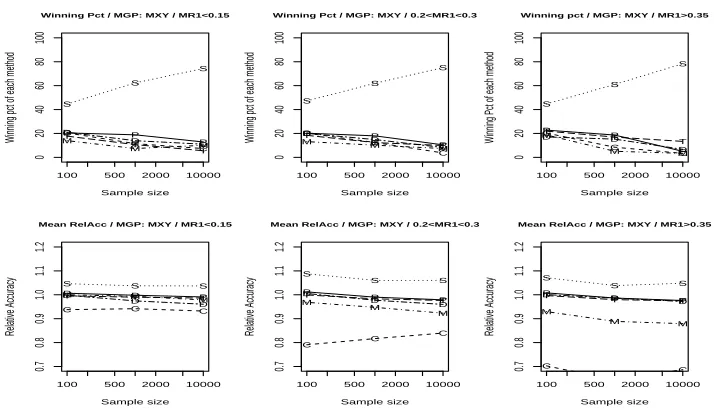
Figure 7: A comparison of the low, median and high missing rate situations. The top row shows the comparison in terms of winning percentage and the bottom row shows the comparison of the absolute performance of each missing data method.
Figure 6 shows the relationship between MR1 and MR2in the simulations with 12 continuous
predictors and 6 of them with missing values. Notice that in this setting, MR1 is naturally between
0 and 0.5 (since half of the predictors can have missing values). MR2values are considerably larger
than MR1values, as would be expected.
The simulations clearly show that the relative performance of different missing data methods is very consistent regardless of the missing rate (see the top row of Figure 7). However, the bottom row of Figure 7 shows that the absolute performance of the complete case method and the mean imputation method deteriorate as the missing rate gets higher. It also shows that separate class method performs best when the missing rate is neither too high or too low, although this effect is relatively small. Interestingly, the relative accuracy of the other missing data methods is very close to one regardless of the missing rate, indicating that they can almost achieve the same accuracy as if the data are complete without missing values.
P
P
P 100 500 2000 5000
0 20 40 60 80 100
Winning pct / MGP: MXY / 0.55<Orig. AUC<0.6
Sample size
Winning pct of each method
C C C S S S M M M T T T D D D P P P
100 500 2000 5000
0 20 40 60 80 100
Winning pct / MGP: MXY / 0.7<Orig. AUC<0.8
Sample size Winning pct of each method C
C C S S S M M M T T T D D D P P P
100 500 2000 5000
0 20 40 60 80 100
Winning pct / MGP: MXY / Orig. AUC>0.9
Sample size
Winning pct of each method
C C
C
S S
S
M M M
T T
T D
D
D
P P P
100 500 2000 5000
0.7 0.8 0.9 1.0 1.1 1.2
Mean RelAcc / MGP: MXY / 0.55<Orig. AUC<0.6
Sample size Relative Accuracy C C C S S M M M T T T
D D D P P
P
100 500 2000 5000
0.7 0.8 0.9 1.0 1.1 1.2
Mean RelAcc / MGP: MXY / 0.7<Orig. AUC<0.8
Sample size Relative Accuracy C
C C S S S M M M
T T T
D
D D
P P P
100 500 2000 5000
0.7 0.8 0.9 1.0 1.1 1.2
Mean RelAcc / MGP: MXY / Orig. AUC>0.9
Sample size Relative Accuracy C C C S S S
M M M
T T T
D D D
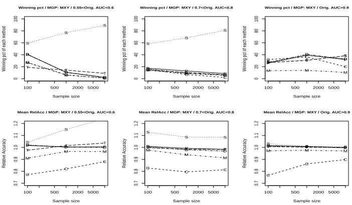
Figure 8: A comparison of the low, median and high original full data AUC situations. The top row shows the comparison in terms of winning percentage and the bottom row shows the comparison of the absolute performance of each missing data method.
3.2.4 THEIMPACT OF THEORIGINALFULLDATAAUC
Figure 8 shows that the original full data AUC primarily has an impact on the performance of separate class method. When the original full data AUC is higher, the loss in information due to missing values is less likely to be compensated by the information in the missingness, and thus separate class method deteriorates in performance (see the bottom row of Figure 8). When the original AUC is very high, although separate class still does a little better on average, it loses the dominance over the other methods.
Another observation is that the missing data methods other than separate class have fairly stable relative accuracy, with complete case and mean imputation consistently being the poorest perform-ers (see the graphs in the bottom rows of both Figure 7 and Figure 8). This is true regardless of the AUC or the missing rate, even when the missingness does not depend on the response variable and there are no missing data in the testing set where, in theory, the complete case method can eventually recover the DGP.
4. Performance On Real Data Sets
In this section, we show that most of the previously described results hold when using real data sets. Moreover, we propose a method of determining the best missing data method to use when analyzing a real data set. Unlike in the previous sections, in these simulations based on real data, default settings of C4.5 are used and RPART is tuned (primarily using its parameter “cp”) to get similar performance on the original full data asC4.5. Therefore, in particular, the effect of pruning
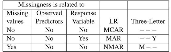
Missingness is related to Missing Observed Response
values Predictors Variable LR Three-Letter
No No No MCAR − − −
No No Yes MAR − −Y
Yes No No NMAR M− −
Table 2: Three missingness patterns used in simulations based on real data sets. The LR column shows the categorization according to Rubin (1976) and Little and Rubin (2002). The Three-Letter column shows the categorization used in this paper.
data sets that contain missing values (since in that case the true missingness generating process is not known by the data analyst).
4.1 Results on Real Data Sets with Simulated Missing Values
The same 36 data sets as in Perlich, Provost, and Simonoff (2003) are used here (except for Cover-type and Patent, which are too big forRPARTto handle; in those cases a random subset of 100,000 observations for each of them was used as the “true” underlying data set). They are either complete or were made complete by Perlich et al. (2003). Missing values with different missingness patterns were generated for the purpose of this study. According to the earlier results, the only important factor in the missingness generating process is the relationship between the missingness and the response variable. Therefore, two missingness patterns are included. In one of them, missingness is independent of all of the variables (including the response variable). In the other one, missingness is related to the response variable, but independent of all of the predictors. These two missingness pat-terns can be categorized as missing completely at random (MCAR) and missing at random (MAR), respectively. To account for this categorization of MGPs, the third type of missingness, not missing at random (NMAR), is also included. In the NMAR case, missingness is made dependent upon the missing values but not on the response variable (see Table 2). To maximize the possible effect of missing values, the first split variable of the original full data is chosen as the variable that contains missing values. It can be either numeric or categorical (binary or multi-categorical). Ten new data sets with missing values are generated for each combination of data set, training set size, and miss-ingness pattern combination, with the missing rate chosen randomly for each. The performance of the missing data methods is measured out-of-sample, on a hold out test sample.
Figure 9: A tally of the relative out-of-sample performance measured in accuracy of all of the miss-ing data methods on the 36 data sets.
4.1.1 THETWO FACTORS AND THEBESTMISSINGDATAMETHOD
Consistent with the earlier results, the two factors that differentiate the performance of different missing data methods are whether the testing set is complete and whether the missingness is depen-dent upon the response variable. Figure 9 summarizes the relative out-of-sample performance in terms of accuracy of all of the missing data methods under different situations. In the graph, each bar represents one missing data method. Since the complete case method is consistently the worst method, it is omitted in the comparisons. Within each bar, the blank block shows the frequency that the missing data method has comparable performance with others. The shadowed block on the bottom shows the frequency that the missing data method has worse performance than others. The line-shadowed blocks on the top show the frequency that the missing data method has better performance than others, with the vertically line-shadowed block further indicating that the missing data method has better performance than with the original full data.
and the response variable because both the missingness and the response variable are related to the predictor.
However, the dominance of probabilistic split is not observed in these real data sets. One pos-sible reason could be the effect of pruning, which is used in these real data sets. The other two methods realized using C4.5 (imputation and separate class) both work with “filled-in” data sets, while probabilistic split takes the missing values as-is. Given this, we speculate that the branches with missing values are more likely to be pruned under probabilistic split, which causes it to lose predictive power. Another possible reason could be the competition from surrogate split, which is realized using RPART. Although we tried to tune RPART for each data set and each sample size, RPARTandC4.5 are still two different algorithms. Different features ofRPARTandC4.5, other than the missing data methods, may cause RPART to outperformC4.5. Complete variable method per-forms a bit worse than the others, presumably because in these simulations the initial split variable on the full data was used as the variable with missing values.
In addition to accuracy, AUC was also tested as an alternative performance measure. We also examined the use of bagging (bootstrap aggregating) to reduce the variability of classification trees (discussion of bagging can be found in many sources, for example, Hastie et al. 2001). The learning curve effect (that is, the relationship between effectiveness and sample size) is also examined. We see patterns consistent with those in the simulated data sets. That is, the relative performance of the missing data methods is fairly consistent across different sample sizes.
4.1.2 THEEFFECT OFMISSINGRATE
Figure 10 shows the distribution of the generated missing rates in these simulations. Recall that missing values occur in one variable, so this missing rate is the percentage of observations that have missing values, that is, MR2as defined earlier. Figure 11 shows a comparison between the case when
the missing rate is low (MR2<0.2) and the case when the missing rate is high (MR2>0.8). For
brevity, only the result when the MGP is dependent on the response variable is shown; differences between the low and high missing rate situations for other MGP’s are similar. Since the missing rate is chosen at random, some of the original data sets do not have any generated data sets with simulated missing values with low missing rate, while for others we do not have any with high missing rate, which accounts for the “no data” category in the figures. Also, when the missing rate is high, the complete case method is obviously much worse than other missing data methods, and is therefore omitted from the comparison in that situation.
By comparing the graphs in Figures 11 with the corresponding ones in Figure 9, we can see some of the effects of missing rate. First, when the missing rate is lower than 0.2, the complete case method has comparable performance to other methods other than the complete variable method. This is unsurprising, as in this situation the complete case method does not lose much information from omitted observations. Secondly, the complete variable method has the worst performance when the missing rate is low, presumably (as noted earlier) because the complete variable method omits the most important explanatory variable in these simulations.
Distribution of missing rates in the simulation on 36 real data sets
Missing Rate
Density
0.0 0.2 0.4 0.6 0.8 1.0
0.0
0.2
0.4
0.6
0.8
1.0
1.2
1.4
Figure 10: The distribution of missing rate in the simulation on 36 real data sets.
Figure 11: A comparison of the relative out-of-sample performance with low and high missing rates. Shown here, as an example, is the relative performance when the missingness is dependent upon the response variable. The left column is for the cases where the test set is fully observed and the right column for the cases where the test set has missing values. Top row shows the cases with low missing rate (MR2<0.2) and bottom row
shows the cases with high missing rate (MR2>0.8)
.
Figure 12: A tally of the missing data methods performance differentiation by data separability (measured by AUC).
4.1.3 IMPACT OF THEDATASEPARABILITY, MEASURED BYORIGINALFULLDATAAUC
The experiment with these 36 data sets also shows that data separability (measured by AUC) is in-formative about the performance differentiation between different missing data methods (see Figure 12). In the graph, each vertical bar represents one of the 36 data sets, which are ordered from left to right according to their maximum full data AUC (as calculated by Perlich et al. 2003) from small-est to the greatsmall-est. The X -axis label shows the AUCs of the data sets. The height of each black bar shows the percentage of time when all of the missing data methods have mostly tied performance on the data set. The percentage is calculated as follows. There are three simulated missingness patterns (MCAR, NMAR and missingness depending on Y ), four different testing sets (complete training set, complete new test set, incomplete training set and incomplete new test set) and four performance measures (accuracy, AUC and their bagged versions). This yields 48 measurement blocks for each data set. The performances of all of the missing data methods are compared within each block. If within a block, all of the missing data methods have very similar performance, the block is marked as mostly tied. Otherwise, the block is marked as having at least one method performing differently. The percentage is the proportion of the 48 blocks that are marked as mostly tied.
4.2 A Real Data Set With Missing Values
We now present a real data example with naturally occurred missing values. In this example, we try to model a company’s bankruptcy status given its key financial statement items. The data are annual financial statement data and the predictions are sequential. That is, we build the tree on one year’s data and then test its performance on the following year’s data. For example, we build a tree on 1987’s data and test its performance on 1988’s data, then build a tree on 1988’s data and test it on 1989 data, and so on.
The data are retrieved from Compustat North America (a database of U.S. and Canadian funda-mental and market information on more than 24,000 active and inactive publicly held companies). Following Altman and Sabato (2005), twelve variables from the data base are used as potential pre-dictors: Current Assets, Current Liabilities, Assets, Sales, Operating Income Before Depreciation, Retained Earnings, Net Income, Operating Income After Depreciation, Working Capital, Liabili-ties, Stockholder’s Equity and year. The response variable, bankruptcy status, is determined using two footnote variables, the footnote for Sales and the footnote for Assets. Companies with remarks corresponding to “Reflects the adoption of fresh-start accounting upon emerging from Chapter 11 bankruptcy” or “Company in bankruptcy or liquidation” are marked as bankruptcy. The data in-clude all active companies, and span 19 years from 1987 to 2005. There are 177560 observations in the original retrieved data, but 76504 of the observations have no data except for the company identifications, and are removed from the data set, resulting in 99056 observations. There are 19238 (19.4%) observations containing missing values and there are 56820 (4.8%) missing data values.
According to the results in Sections 3 and 4.1, there are two criteria that differentiate the per-formance of different missing data methods, that is, whether or not there are missing values in the testing set and whether or not the missingness depends on the response variable. In the bankruptcy data, there are missing values in every year’s data, and thus missing values in each testing data set. To assess the dependence of the missingness on the response variable, the following test is carried out. First, we define twelve new binary missingness indicators corresponding to the original twelve predictors. Each indicator takes on value 1 if the original value for the associated variable is missing and 0 if the original value is observed for that observation. We then build a tree for each year’s data using the indicators as the predictors and the original response variable, the bankruptcy status, as the response variable. From 1987 to 2000, the tree makes no split, indicating the tree algorithm is not able to establish a relationship between the missingness and the response variable. From 2001 to 2005, the classification tree consistently splits on the missingness indicators of Sales and Re-tained Earnings. This indicates that the missingness of these predictors has information about the response variable in these years, and the MGP across the years is fairly consistent in missingness in sales and retained earnings being related to bankruptcy status. However, the AUC values calculated from the trees built with the missingness indicators are not very high, all being between 0.5 and 0.6. Therefore, the relationship is not a very strong one.
rpart accuracy, missingness indep of response
year
Accuracy
1988 1990 1992 1994 1996 1998 2000
0.980
0.990
1.000
C4.5 accuracy, missingness indep of response
year
Accuracy
1988 1990 1992 1994 1996 1998 2000
0.980
0.990
1.000
rpart accuracy, missingness dep on response
year
Accuracy
2002 2003 2004 2005
0.980
0.990
1.000
C4.5 accuracy, missingness dep on response
year
Accuracy
2002 2003 2004 2005
0.980
0.990
1.000
rpart TP, missingness indep of response
year
True Positive Rate
1988 1990 1992 1994 1996 1998 2000
0.0 0.1 0.2 0.3 0.4 0.5
C4.5 TP, missingness indep of response
year
True Positive Rate
1988 1990 1992 1994 1996 1998 2000
0.0 0.1 0.2 0.3 0.4 0.5
rpart TP, missingness dep on response
year
True Positive Rate
2002 2003 2004 2005
0.0 0.1 0.2 0.3 0.4 0.5
C4.5 TP, missingness dep on response
year
True Positive Rate
2002 2003 2004 2005
0.0 0.1 0.2 0.3 0.4 0.5
Figure 13: The relative performance of all of the missing data methods on the bankruptcy data. The left column gives methods using RPART (and includes all of the methods except for probabilistic split) and the right column gives methods usingC4.5 (and includes all of the methods except for surrogate split). The top rows are performance in terms of accuracy while the bottom rows are in terms of true positive rate.
the missing data methods except for probabilistic split. The plots on the right are the results from
C4.5, which include all of the missing data methods except for surrogate split. The performances of methods common to both plots are slightly different because of differences between C4.5 and
RPARTin splitting and pruning rules. Both the accuracy and the true positive rates are shown. Since the number of actual bankruptcy cases in the data is small, the accuracy is always very high. The true positive rate is defined as
T P=Number of correctly predicted bankruptcy cases Actual number of bankruptcy cases .
The graphs in the first and the second rows are for accuracies, with the first row for the first time period from 1988 to 2001 and the second row for the second time period from 2002 to 2005. The graphs in the third and the fourth rows are for true positive rates, with the third row for the first time period from 1988 to 2001 and the fourth row for the second time period from 2002 to 2005. It is apparent that in the first time period, there are no clear winners. However, in the second time period, separate class is a little better than the others, in line with expectations.
5. Extension To Logistic Regression
One obvious observation from this study is that when missing values occur in both the model build-ing and model application stages, it should be considered as part of the data generatbuild-ing process rather than a separate mechanism. That is, taking the missingness into consideration can improve predictive performance, sometimes significantly. This should also apply to other supervised learn-ing methodologies, non-parametric or parametric, when predictive performance is concerned. We present here the results from a real data analysis study involving logistic regression, similar to the one presented in Section 4.1. Missing values are generated the same way as in Section 4.1 and then logistic regression models (without variable selection) with different ways of handling missing data are applied to those data sets. Finally a tally is made on the relative performances of different missing data methods. Results measured in accuracy, bagged accuracy, AUC and bagged AUC are almost identical to each other; results in terms of accuracy are shown in Figure 14.
Included in the study are five ways of handling missing data: using only complete cases (com-plete case method), including a missingness dummy variable in the explanatory variable (dummy method, sometimes called the missing-indicator method),1 building separate models for data with values missing and data without missing values (by-group method),2imputing missing values with grand mean/mode (imputation method), and only using predictors without missing values (complete variable method). Note that the methods using a dummy variable and building separate models for
1. If explanatory variable X1has missing values, then we create a missingness dummy variable M1that has value 1 if X1
is observed and 0 otherwise. Then M1and X1∗M1are both used as explanatory variables. The result of this set-up
is that the effect of X1is fit on the observations with X1observed but a single mean value is fit to the observations
with X1missing. All of the observations, with or without X1values, have the same coefficients for all of the other
explanatory variables. Jones (1996) showed that this method can result in biased coefficient estimates in regression modeling, but did not address the question of predictive accuracy that is the focus here.
Figure 14: A tally of the relative out-of-sample performance with logistic regression measured in accuracy of all of the missing data methods on the 36 data sets.
observations with and without missing values each are analogous to the separate class method for trees. The most obvious observation is that when missingness is related to the response variable and missingness occurs in the test set, the dummy method and the by-group method dominate the other methods; in fact, more than a third of the time, they perform better than logistic regression on the original full data. Comparing Figure 14 with Figure 9, we see a clear similarity, in that the meth-ods using a separate class model missingness directly, and thus use the information contained in the missingness about the response variable most efficiently. This suggests that the result that predictive performance of supervised learning methods is driven by the dependence (or lack of dependence) on the response variable is not limited to trees, but is rather a general phenomenon.
6. Conclusion And Future Study
The main conclusions from this study are as follows:
1. The two most important criteria that differentiate the performance of different missing data methods are whether or not the testing set is complete and whether or not the missingness depends on the response variable. There is strong evidence, both analytically and empirically, that separate class is the best missing data method to use when the testing data also contains missing values and the missingness is dependent upon the response variable.
the missingness indicators (which equals to 1 if the corresponding original value is missing and 0 otherwise). If such a model supports a relationship, then it is an indication that the missingness is related to the response variable.
2. The performance of classification trees is on average not too negatively affected by missing values, except for the complete case method and the mean imputation method, which are sensitive to different missing rates. Separate class tend to perform better when the missing rate is neither too high nor too low, trading off between information loss due to missing values and information gain from the informative MGP.
3. The original full data AUC has an impact on the performance of separate class method. The higher the original AUC, the more severe the information loss due to missing value, and thus relatively the worse the performance of the separate class method.
The consistency of these results across the theoretical analyses, simulations from the artificial data, and simulations based on real data provides strong support for their general validity.
The findings here also have implications beyond analysis of the data at hand. For example, since missingness that is dependent on the response variable can actually improve predictive performance, it is clear that expending time, effort, and money to recover the missing values is potentially a poor way to allocate resources. Another interesting implication of these results is related to data disclo-sure limitation. It is clear that any masking of values must be done in a way that is independent of the response variables of interest (or any predictors highly related to such variables), since otherwise data disclosure using regression-type methods (Palley and Simonoff, 1987) could actually increase. Classification trees are designed for the situation where the response variable is categorical, not just binary; it would be interesting to see how these results carry over to that situation. Tree-based methodologies for the situation with a numerical response have also been developed (i.e., regression trees), and the problems of missing data occur in that context also. Investigating such trees would be a natural extension of this paper. In this paper, we focused on base form classification trees usingC4.5 andRPART, although bagging was included in the study. It would be worthwhile to see how the performance of different missing data methods is affected by different tree features such as stopping and pruning or when techniques such as cross-validation, tree ensembles, etc. are used.
Moreover, as was shown in Section 5, the relationship between the missingness and the response variable can be helpful in prediction when missingness occurs in both the training data and the testing data in situations other than classification trees. This is very likely true for other supervised learning methods, and thus testing more learning methods would also be a natural extension to this study.
Acknowledgments
P(Y =0|X=0,with Missing Data) >T >T
P(Y =0|X=1,with Missing Data) >T ≤T
P(Y=0|X=0) P(Y=0|X=1)
>T >T 1 P(X=0,Y=P0()+Y=P0()X=1,Y=1)
>T ≤T P(X=0,Y=P0(Y)+=P0()X=1,Y=1) 1
≤T >T P(X=0,Y=P1(Y)+=P0()X=1,Y=0) PP((XX==00,,YY==10)+)+PP((XX==11,,YY==10))
≤T ≤T PP((YY==01)) P(X=0,Y=P0()+Y=P1()X=1,Y=1)
P(Y =0|X=0,with Missing Data) ≤T ≤T
P(Y =0|X=1,with Missing Data) >T ≤T
P(Y=0|X=0) P(Y=0|X=1)
>T >T P(X=0,Y=P1()+Y=P0()X=1,Y=0) PP((YY==10))
>T ≤T PP((XX==00,,YY==10)+)+PP((XX==11,,YY==01)) P(X=0,Y=P0()+Y=P1()X=1,Y=1)
≤T >T 1 P(X=0,Y=P1()+Y=P1()X=1,Y=0) ≤T ≤T P(X=0,Y=P1()+Y=P1()X=1,Y=0) 1
Table 3: RelAcc of tree built on data with missing values and tested on the original full data set when there is no variation from true DGP
Appendix A. Proofs of the Theorems
The relative accuracy (RelAcc) when there are missing values in the training set but not in the testing set can be summarized into Table 3, where T is the threshold value (an observation will be classified as class 0 if the predicted probability for it to be 0 is greater than T ). The value of T reflects the misclassification cost. It is taken as 0.5 reflecting an equal misclassification cost. In Table 3, the columns show different rules given by the classification trees when there are missing values, and the rows show actual DGP’s. The entries are the RelAcc values under different scenarios. For example, all of the entries on the diagonal are one’s because the rules given by the classification trees when there are missing values are the same as the true DGP’s and thus the accuracy achieved by the trees are the same with or without the missing values and thus RelAcc=1. Cell(1,2), for example, shows that if the true DGP is P(Y =0|X =0)>T and P(Y =0|X =1)>T but the classification
tree gives rule P(Y =0|X=0)>T and P(Y =0|X =1)≤T when there are missing values, that
is, P(Y =0|X=0,with missing value)>T and P(Y =0|X =1with missing value)≤T , then the
relative accuracy is determined to be
P(X=0,Y =0) +P(X=1,Y =1)
P(Y=0) .
Proof of Theorem 1 : The expected performance of the complete case method when the
missing-ness does not depend on the response variable and the testing set is complete.
Proof
contain missing values in any of the predictors. Y is the response variable and X is the vector of the predictors.
If only the complete cases are used, if P(Y|A=0,X) =P(Y|X), then only the diagonal in Table 3 can be achieved, and thus there is no loss in accuracy.
This condition will be satisfied if and only if the MGP is conditionally independent of Y given
X , that is, P(A=0|X,Y) =P(A=0|X).
1. “P(Y|A=0,X) =P(Y|X)⇒P(A=0|X,Y) =P(A=0|X)”
P(A=0|X,Y)= P(AP=(X0,,YX),Y) =P(Y|A=P0,(XX),PY()A=0,X) =P(YP|(XY)|PX()AP=(X0),X) =P(A=0|X)
2. “P(Y|A=0,X) =P(Y|X)⇐P(A=0|X,Y) =P(A=0|X)”
P(Y|A=0,X)= P(A=0,X,Y)
P(A=0,X)
=P(A=P0(|AX=,Y0),PX()X,Y) =PP(A(A==00|X|X)P)P(X(X,Y)) =PP(X(X,Y))
=P(Y|X)
Proof of Theorems 2 and 3 : The expected performance of the complete case method when the
missingness depends on the response variable and the testing set is complete.
We first observe the following lemmas.
Lemma 7 For the partition defined by the tree built on the original full data (and not changed
by missing values), let the kthsection contain Pk proportion of data and within the partition,
the majority class have proportion Pm jk . Note that∑Kk=1Pk=1, while the full data set
accu-racy, that is, the accuracy achievable with the full data set, is∑kPkPm jk .)
The rule for the kth section will be classifying it as the majority class of the section. The
impact of missing data on its rule is to either leave it unchanged or make it classify the data as the minority class instead of the majority class.
The smallest missing rate needed in kthsection to change the rule is P(A=1|k) =2Pm jk −1,
where A is defined as in Theorem 1, that is, it is the case-wise indicator, which takes value 1 if the observation contains missing value or 0 otherwise. If the rule is changed the loss in