Vol. 13, 2018, 13-19
ISSN: 2349-0632 (P), 2349-0640 (online) Published 1 April 2018
www.researchmathsci.org
DOI: http://dx.doi.org/10.22457/jmi.v13a2
13
Journal of
Time Minimizing Multi-Index Bulk Transportation
Problem
Sungeeta Singh1, Sudhir Kumar Chauhan2 and Kuldeep3 1
Department of Mathematics, Amity University, Gurugram Haryana, India. E-mail: [email protected] 2
Department of Mathematics, Amity School of Engineering and Technology Bijwasan, New Delhi, India. E-mail:[email protected]
3
Department of Mathematics, Amity University Gurugram, Haryana, India. E-mail: [email protected]
3
Corresponding Author
Received 1 March 2018; accepted 28 March 2018
Abstract. In industries, usually, two or more than two types of commodities are manufactured to maximize the profit. Sometimes, commodities are supplied to multiple warehouses via different modes of transportation. To deal such type of problems in transportation, transportation problems are extended into Multi-Index Transportation Problems(MITP). In this paper, Multi-Index Bulk Transportation problem(MIBTP) which is anextension of Bulk Transportation Problem(BTP) having two modes of transportation with time minimizing objective is considered.In the present paper, VAM is extended to study the time minimizing MIBTP already studied by Latha [23] and a comparative study is done on the existing method and proposed amethod.
Keywords: Transportation, Bulk Transportation, Multi-Index Bulk Transportation AMS Mathematics Subject Classification (2010): 90C08
1. Introduction
Transportation model is a special class of the linear programming problem that deals with the distribution ofnumber of units of a commodityfrom multiple warehouses to multiple destinations satisfying supply and demand constraints with cost minimizing objective. Transportation model plays an important role in supply-chain management and logistics for reducing the cost of transportation in industries. The classical transportation problem was presented first by Hitchcock [1]. Later on, Koopmans [2] and Dantzig [3] further developed the theory of transportation problem. Several other authors, like, Balas [4], Bhatia et al. [5], Hammer [6], Szwarc [7], Hakim [8], Ahmed et al. [9] and Pramila and Uthra [10] using different approaches for solving the transportation problems.
14
ofnumber of units of the product. Maio and Roveda [11] were the first who presented the theory of BTP with cost minimizing objective. The authors solved the problem by an iterative procedure. Later on, Srinivasan and Thompson[12] presented an algorithm based on branch and bound method for solving the earlier problem. Several other authors like Bhatia [13], Foulds and Gibbons [14] and Verma and Puri [15] studied the different BTPusing different approaches.
To maximize the profit, generally, two or more than two types of products are manufactured in factories and transported to various destinations to meet their requirements. Sometimes, products are supplied to various destinations through different modes of transportation.To optimize the profit in all such cases, transportation problems are extended intoMITP. The problem is extended into MITP by considering commodities or modes of transportation as additional indices.MITP was first introduced by Schell [16] and Galler and Dwyer [17] in literature. Several other authorslike Haley [18], Junginer [19], Korsnikov [20], Pandian and Anuradha [21], Patel and Tripathy [22] studied MITP using different approaches. Latha [23] studied MIBTP with time minimizing objective using Lexi-Search algorithm.
In the present paper, the MIBTP solved by Latha [23] is considered and an algorithm is proposed for minimizing thetime of MIBTP. In Section 2, the formulation of the problem is discussed and in Section 3, steps of the proposed algorithm are presented. In Section 4, a numerical example is worked out to illustrate the proposed algorithm. Finally, in section 5, theconclusion is presented.
2. Formulation of the problem
Let there are‘m’ sources producing a certain product and ‘n’ destinations having some requirements. Let the products are supplied to multiple destinations through two modes of transportation to meet their requirements.Let ‘T’ denotes the total time of MIBTP. The mathematical formulation of time minimizing MIBTP is as follows:
Minimize
= max{ : = 1, = 1,2, … , ; = 1,2, … . , ; = 1,2} (1)
subject to the constraints ∑ ∑ ≤ (2)
∑!∑ = 1 (3)
= 1 #$ 0 (4)
&&&= '''= 1 for = , ≠ ) ≠ (5)
where , ) are non-negative real numbers.
Here ‘’ and‘’ denote the amount of product available at the th source and
15 3. Proposed solution procedure
The proposed solution procedure comprises two main steps. In step 1, an algorithm is separately proposed for solving the bulk transportation problems for each mode of transportation. Step 2 provides theminimumtime of MIBTP.
Step 1.
(i) Delete the cells (, ) from the table for which number of units of the product available at the ith source is less than the requirement of jth destination.
(ii) Select the two lowest bulk transportation time for each row and column and find their difference. This difference indicates the penalty. This penalty represents an additionaltime which has to be paid if the cell having lowestbulk transportation time remainsunallocated.
(iii) Select the largest penalty among all the penalties so obtained and allocate 1 to the lowesttimecell (, ) corresponding to the largest penalty.This means that requirement of jth destination will be met fromith source. In case of tie among the largest penalties, select thecell (, ) having lowest time. Again, if there is tie, then select the cell (, )for which maximum allocation can be done.
(iv) Decrease the number of units of the product available at the ith
source by the demand ofjth destination whose demand has been met.
(v) Remove the rows from the table having zero availability or which can’t satisfy the requirement of any destination. Also, remove the destinations whose demand has been met.
Repeat steps (i) to (v) until the requirement of all destinations are satisfied. Step 2.Select minimum of the corresponding times associated with the decision variables
through facility k = 1 and k = 2 for each destination. Then, maximum of all such times gives the minimum the time of MIBTP.
4. Numerical problem
The problem studied by Latha [23] is considered here in which there are 3 sources, 5 destinations,and 2 facilities. The availabilities and requirements of the sources and destinations are 25, 30, 35 and 10, 12, 15, 8, 10 respectively.In BTP P1 and P2, bulk times of transportation are given through facility k = 1 and k = 2 respectively. The proposed method is applied to the problem to determine the minimum time of transportation. The tableau representation of the numerical problem is given is given below.
P1 (Representation of times of BTP through 1st facility)
D1 D2 D3 D4 D5 ↓
S1 15 13 7 9 4 25
S2 1 7 12 9 12 30
S3 22 20 6 11 13 35
16
P2 (Representation of times of BTP through 2nd facility)
Applying step 1 for solving the problem .. The penalties for sources/, /and /2 are 3, 6 and 5 respectively and the penalties for destinations 3, 3, 32,34and 35are 14, 6, 1, 0 and 8 respectively. Among these penalties, the largest penalty is 14 corresponding to the destination 3.Lowest time in the column associated with destination 3 is 1 in the cell (2, 1) , so making allocation atthe cell (2, 1) . 6. = 1. This fulfills the demand of
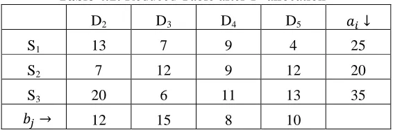
destination 3 . Remove the destination 3 from the table and update the table to obtain Table 4.1
Table 4.1: Reduced Table after 1st allocation
In
Table 4.1, the penalties for sources /, /and /2are 3, 2 and 5 respectively and for
destinations 3,32, 34 and 35 are 6, 1, 0 and 8 respectively. Among these penalties, the largest penalty is8 associated with destination 35. Lowesttime in the column associated with destination 35 is 4 in the cell (1, 5), so select the cell (1, 5). 6. 5= 1. This
fulfills the demand of destination 35.Remove the destination35from the table and update
the table to obtain table 4.2
Table 4.2: Reduced Table after 2nd allocation
In Table 4.2, the penalties for sources /, / ) /2 are 2, 2 and 5 respectively and for
destinations 3, 32 and 34 are 6, 1 and 0 respectively. Among these penalties, the
largestpenalty is 6 associated with destination 3. Lowesttime in the column associated
with destination 3 is 7 in the cell(2, 2), so making allocation at the cell
(2, 2) . 6. = 1. This fulfills the demand of destination 3. Remove the destination
D1 D2 D3 D4 D5 ↓
S1 9 1 3 8 12 25
S2 7 10 12 5 4 30
S3 3 18 4 2 14 35
→ 10 12 15 8 10
D2 D3 D4 D5 ↓
S1 13 7 9 4 25
S2 7 12 9 12 20
S3 20 6 11 13 35
→ 12 15 8 10
D2 D3 D4 ↓
S1 13 7 9 15
S2 7 12 9 20
S3 20 6 11 35
17
3 from the table. Further,since the remaining availability of the source S2 is less than the
requirement of destination D3, deleting the entry of the cell (2, 3), we have the reduced Table 4.3.
Table 4.3: Reduced Table after 3rd allocation
In Table 4.3, the penalties for sources /, / and /2 are 2, 9 and 5 respectively and for destinations 32 and 34 are 1 and 0 respectively. Among these penalties, the highest
penalty is 9 associated with source /. Lowest time in the row associated with source /
is 9 in the cell (2,4), so making an allocation at the cell (2, 4) . 6. 4= 1. This fulfills
the demand of destination 34 and this also exhausts the availability of source /.
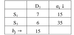
Remove the destination 34 and source the/from the table, we have the reduced Table 4.4.
Table 4.4: Reduced Table after 4th allocation
In Table 4.4, the penalties for sources / and /2 are 7 and 6 respectively and for destination 32 is 1. Among these penalties, the largest penalty is 7 associated with source
/. Lowest time in the rowassociated with source/ is 7 in the cell (1,3). So, making
allocation in the cell (1,3), . 6. 2= 1. This satisfies the demand of destination 32.
Thus, all destinations met their demands. The decision variables which assume value 1 for the BTP P1 are , , 2, 4 and 5. Similarly, on solving the second BTP P2 satisfying all the constraints, we have the decision variables which assume value 1 are 2, , 22, 4 ) 5. The following table gives the allocations through facility k=1 & k=2 and the final solution of the considered problem.
Table 4.5: Optimal solution of the MIBTP Decision variables
through facility k=1 and associated time
Decision variables through facility k=2 and associated time
Minimum of the corresponding timesassociated with decision variables through facility k=1 & k=2 and associated decision variables
, = 1
, = 7
2, 2 = 7
2, 2= 3
, = 1
22, 22= 4
= 1,
= 1,
22= 4, 22
D3 D4 ↓
S1 7 9 15
S2 - 9 8
S3 6 11 35
→ 15 8
D3 ↓
S1 7 15
S3 6 35
18
4, 4= 9
5, 5 = 4
4, 4= 5
5, 5= 4
4= 5, 4
5= 4, 5
Thus, the solution of the considered MIBTP is < = {, , 22, 4, 5} and the minimum time of MIBTP is T = Max {1, 1, 4, 5, 4} = 5.
Table 4.6: Comparative study Decision variables and Optimal time of
MIBTP by the method proposed by Latha [23]
Decision variables and Optimal time of MIBTP by the proposed method
, , 22, 4, 5 and T = 5 , , 22, 4, 5and T = 5
Thus, we observe that the proposed method provides the same optimal solution as provided by Latha [23]. However, the proposed method is much simpler as compared toLexi-Search algorithm based upon pattern recognition technique proposed by Latha [23].
5. Conclusion
In the present paper, MIBTP already solved by Latha [23] is considered and is solved by the proposed method which gives the same optimal solution as by Latha [23]. Latha [23] used Lexi- Search algorithm based on pattern recognition technique to solve the problem. But, the method in this paper is quite simple as compared to theLexi-Search algorithm as it involves a less number of calculations.Also, the proposed method is very easy to apply on the problem and an alternative method for solving the time minimizing MIBTP.
Acknowledgement. The authors would like to thank the anonymous reviewers for their valuable comments on the paper, as these comments led us to an improvement of the work.
REFERENCES
1. F.L.Hitchcock, The distribution of a product from several sources to numerous locations, Journal of Mathematics and Physics, 20 (1941) 224-230.
2. T.C.Koopmans, Optimum utilization of Transportation System, Econometrica supplement, 17(1949).
3. G.B.Dantzig, Linear Programming and Extensions, Princeton University Press, Princeton, New Jersey, 1963.
4. E.Balas, An additive algorithm for solving linear programs with zero-one variables, Operation Research, 13 (1965) 517-545.
5. H.L.Bhatia, M.C.Puri and K.Swarup, A procedure for time minimizing transportation problem, Indian Journal of Pure & Applied Mathematics, 8 (1977) 920-929.
6. P.L.Hammer, Time minimizing transportation problems, Naval Research Logistics Quarterly, 16 (1970) 345-357.
19
8. M.A.Hakim, An alternative method to find initial basic feasible solution of a transportation problem, Annals of Pure and Applied Mathematics, 1 (2012) 203-209. 9. M.M.Ahmed, A.S.Muhammad Tanvir, S.Sultana, S.Mahmud and Md. S.Uddin, An
effective modification to solve transportation problems: a cost minimization approach, Annals of Pure and Applied Mathematics, 6 (2014) 199-206.
10. K.Pramila and G.Uthra, Optimal solution of an intuitionistic fuzzy transportation problem, Annals of Pure and Applied Mathematics, 8 (2014) 67-73.
11. A.D.Maio and C.Roveda, An all zero-one algorithm for a certain class of transportation problems, Operations Research, 19 (1971) I406-1418.
12. V.Srinivasan and G.L.Thompson, An algorithm for assigning users to sources in a special class of transportation problems, Operations Research, 21 (1973) 284-295. 13. H.L.Bhatia, A Note on a zero-one time minimizing transportation problem, NZOR, 7
(1979) 159-165.
14. L.R.Foulds and P.B.Gibbons, New algorithms for the bulk zero-one time mini-max transportation model, NZOR, 8 (1980) 109-119.
15. V.Verma and M.C.Puri, A branch and bound method for cost minimizing Bulk transportation problem, Opsearch, 33 (1996) 145-161.
16. E.D.Schell, Distribution of a product of several properties, In Proc. 2nd Symposium in Linear Programming, pp. 615–642. DCS/ controller, H.Q. U.S. Air Force Washington, D.C, 1955.
17. B.Galler and P.S.Dwyer, Translating the method of reduced matrices to machines, Naval Res. Logistics, 4 (1957) 55-71.
18. K.B.Haley, The multi-index problem, Operation Research, 11 (1963) 368–379. 19. W.Junginer, On representatives of multi-index transportation problems, European
Journal of Operational Research, 66 (1993) 353-371.
20. A.D.Korsnikov, Planar three index transportation problems with dominating index, Mathematical Methods of Operations Research, 32 (1988) 29–33.
21. P.Pandian and G.Anuradha, A new approach for solving solid transportation problems, Applied Mathematical Sciences, 4 (2010) 3603-3610.
22. G.Patel and J.Tripathy, The solid transportation problem and its variants, International Journal of Management and Systems, 5 (1989) 17-36.