A Comparative Study of Some Optimization Methods with the Best Candidate Method for Fuzzy Transportation Problem

(1)

Vol. 15, No. 1, 2017, 77-88

ISSN: 2279-087X (P), 2279-0888(online) Published on 11 December 2017

www.researchmathsci.org

DOI: http://dx.doi.org/10.22457/apam.v15n1a7

77

Annals of

A Comparative Study of Some Optimization Methods

with the Best Candidate Method for Fuzzy

Transportation Problem

D. Stephen Dinagar1 and R.Keerthivasan2

1

PG and Research Department of Mathematics

T.B.M.L. College, Porayar - 609307, India. e-mail: [email protected] 2

Lecturer, Department of Mathematics, Veludaiyar Polytechnic College Tiruvarur - 613701, India. e-mail: [email protected]

1

Corresponding Author

Received 1 November 2017; accepted 8 December 2017

Abstract. In this paper, the fuzzy transportation problems using interval valued triangular fuzzy number are discussed. The initial basic feasible solution of the same fuzzy transportation problem is obtained by different methods, such as North West corner, North East corner, Least Cost method and Best Candidate Method. Finally comparisons have been made with the Best Candidate Method and other given methods. Numerical illustrations are included to justify the above said notion.

Keywords: Interval valued triangular fuzzy number, north west corner rule, north east corner rule, least cost method and best candidate method.

AMS Mathematics Subject Classification (2010): 90C08 1. Introduction

The transportation problem (TP) is a special class of linear programming problems. In this problem a product is to be transported from m sources to n designations and their capacities are a1.a2...am and b1, b2...bn respectively. In addition there is a penalty cij associated with transporting unit of product from source i to designations j. This penalty may be cost or delivery time or safety of delivery etc. A variable xij represents the unknown quantity to be shipped from source i to destination j. The transportation problem, in which the transportation costs, supply and demand quantities are represented in terms of fuzzy numbers, is called a fuzzy transportation problem. The objective of the fuzzy transportation problem is to determine the transportation schedule that minimizes the total fuzzy transportation cost while satisfying the availability and requirement limits.

(2)

D. Stephen Dinagar and R.Keerthivasan

78

by Saad and.Abbas [5]. Nagoorgani and Abdul Razak [1] obtained a fuzzy solution for a Two Stage with trapezoidal fuzzy numbers. Dinagar and Keerthivasan [3] obtained a fuzzy solution with Best Candidate Method using interval valued triangular fuzzy number.

In this work , the fuzzy transportation problems using interval valued triangular fuzzy numbers have been discussed the initial basic feasible solution of the same transportation problem is obtained by different methods such as North West Corner rule , North East Corner rule , Least cost Method and Best Candidate Method.

The rest of this paper is structured as follows. In the next section , We introduce some basic concepts related to interval valued triangular fuzzy number and some operational laws of interval valued triangular fuzzy number and study their desirable properties such as addition, subtraction, and multiplication. Methodology is in section 3. Some algorithms of transportation problem is in the section. The numerical examples are presented in section 4. The numerical results are compared with best candidate method in section 5 . Some conclusions are presented in the final section.

2. Preliminaries

In this section the basic concepts of fuzzy sets, fuzzy number, interval valued triangular fuzzy number and its properties, arithmetic operations of interval valued triangular fuzzy number, ranking function of fuzzy number etc. are recalled.

.

Definition 2.1. A fuzzy set Ã, defined on the universal set X is a set of ordered pairs: Ã={( x , µÃ (x)):x ∈ X}.

Definition 2.2. A fuzzy set Ã, defined on the universal set of real numbers R, is said to be a fuzzy number if its membership function has the following characteristics:

1. µÃ: R→[0,1] is continuous

2. µÃ (x)=0 for all x∈ −∞, ∪ , ∞.

3. µÃ (x) is strictly increasing on [a,b] and strictly decreasing on [b,c]. 4. µÃ (x)=1 for all x=b, where a<b<c.

Definition 2.3. An interval – valued fuzzy set Ã defined on R is called the level λ- Triangular fuzzy number if its membership function is

λ

, a ≤ x ≤ b µÃ (x)= λ

, b≤ x ≤ c 0, otherwise

when a < b< c, 0 < λ≤1, then Ã is called the level λ fuzzy number and denoted by Ã = (a,b,c; λ). When λ=1 it is known as triangular fuzzy number and denoted by Ã = (a,b,c).

Definition 2.4. An interval – valued fuzzy set Ã on R is given by Ã = { (x, [µÃL(x), µÃU(x)])}, for all x∈R,0 ≤ µÃ

L

(x) ≤ µÃ U

(x) ≤ 1 And µÃ L

(x) , µÃ U

(3)

for Fuzzy Transportation Problem

79

Definition 2.5. Let ÃL =( a,b,c;λ ) and ÃU =( d,e,f;ρ ) Where 0 < λ≤ρ≤ 1 and d < a , c < f. Then the interval – valued fuzzy set is expressed asÃ = [ (a,b,c;λ), (d,e,f;ρ)]. The family of all level (λ , ρ) interval-valued fuzzy numbers is denoted by FIV (λ , ρ) = {[(a,b,c;λ), ( d,e,f;ρ)]| d<a, c<f}, Where 0 < λ≤ρ≤ 1, a,b,c,d,e,f R

Definition 2.6. The interval-valued fuzzy set Ã indicates that, when the membership grade of X belongs to the interval [µÃL(x), µÃU(x)], the largest grade is µ ÃU

(x)

and the smallest grade is µÃL(x)

λ

, a ≤ x ≤ b Let µÃ

L(x)

= λ

, b ≤ x ≤ c (1) 0, otherwise

Then, ÃL=(a,b,c;λ ), a<b<c.

ρ

, p ≤ x ≤ q Let µÃU(x)= ρ

, q ≤ x ≤ r (2) 0, otherwise

Then, ÃU=( p,q,r;ρ ) , p < q <r.Consider the case in which 0 < λ <ρ ≤ 1 and p<a, c<r from (1) and (2) , we obtain Ã = [ÃL ,ÃU] = [ ( a,b,c; λ) , ( p,q,r; ρ )], which is called the level (λ , ρ) interval valued fuzzy number.

Definition 2.7. Let Ã = [ÃL ,ÃU] = [ ( a1,b1,c1; wÃ) , ( a2, b2, c2; WÃ )], B͂ = [B͂L ,B͂ U] = [ ( p1,q1,r1; wB͂) , ( p2, q2, r2; WB͂ )]∈ FIV (λ , ρ).

Through operations level λ fuzzy numbers and level ρ fuzzy numbers we can get the following:

(i) Addition:

Ã (+) B͂ = [(a1+p1,b1+q1,c1+r1;min { wA͂, wB͂}), (a2+p2,b2+q2,c2+r2;min {WA͂,WB͂})]

(ii) Subtraction:

Ã (-) B͂ = [(a1-r1,b1-q1,c1-p1;min {wA͂,wB͂}), (a2-r2,b2-q2,c2-p2;min { WA͂, WB͂})].

(iii) Multiplication:

Ã (x) B͂ = [(a1.R(B͂ ),b1.R(B͂),c1.R(B͂);min { wA͂, wB͂}),(a2.R(B͂),b2.R(B͂),c2.R(B͂ );min { WA͂,WB͂})] if R(B͂)≥0.

Ã (x) B͂ = [(a3.R(B͂ ),a2.R(B͂),a1.R(B͂);min { wA͂, wB͂}),(a3.R(B͂),a2.R(B͂),a1.R(B͂);min { WA͂,WB͂})] if R(B͂)<0.

where, R(B͂ ) = ( bLl+ b L

2+ b L

3 +b U

l+ b U

2 + b U

3 ) / 6.

3. Methodology

(4)

80

problem. The fuzzy transportation problem was selected from the literature and their initial basic feasible solution were obtained using different methods. Then vogel’s approximation method was used to find out the optimal solution of the test problems, and there results were compared with the true optimal solution .The brief summaries of five methods, namely north west corner rule, north east corner rule, least cost method, vogel’s approximation method and best candidate method are given in this paper.

3.1. Solution of a fuzzy transportation problem Finding an initial basic feasible solution.

Solution Algorithm

STEP 1: Construct the Problem

STEP 2: Determine the points a1, b1, c1; w_Ã , a2, b2, c2; w_Ã and [ ( p1,q1,r1; wB͂) , ( p2, q2, r2; WB͂ )] for the fuzzy number in the formation problem (Two stages FCMTP).

STEP 3: Formulate the problem (Two stage FCMTP) in the parametric form. STEP4: Apply Prescribed method to get the basic feasible solution

STEP5: Declare min(c1+c2) as the optimal value of the objective function of the problem.

4. Example

For a fuzzy transportation problem is given below , find the fuzzy quantity of the product transported from each source to various destinations so that the fuzzy transportation cost is minimum.

Table 4.1:

D1 D2 D3 D4 SUPPLY

S1 7 5 6 4 [(6,10,14,;0.5),(2,8,20;

0.9)]

S2 3 5 4 2 [(10,14,24;0.7),(2,12,3

0;0.9)]

S3 4 6 4 5 [(18,22,26;0.3),(6,20,2

8;0.6)]

S4 8 7 6 5 [(8,12,16,;0.7),(4,10,3

4;0.9)] DEMAN

D

[(4,8,12;0.3,) ,(0,2,22;0.8)]

[(8,12,16;0.6), (6,10,20;1.0)]

[(12,16,22;0.4),(6, 20,32;0.6)]

[(18,22,34;0.8),(2, 18,38;1.0)]

[(42,58,84;0.3),(14,50, 112;0.6)]

Solution :

Since ∑$_#%&_# = ∑)_(%&'₍ , the problem is a balanced fuzzy transportation problem.

4.1. North west corner rule Stage I

We take & = [(3,5,7,;0.5),(1,4,10;0.9)], * = [(5,7,14;0.7),(1,6,15;0.9)]

+= [(9,11,13;0.3),(3,10,14;0.5)], , = [(4,6,8;0.7),(2,5,17,;0.9)] ,

'_& = [(2,4,6;0.3,),(0,1,11;0.8)] , '_* = [(4,6,8;0.6), (3,5,10;1.0)],

(5)

81 Table 4.1.1:

D1 D2 D3 D4 SUPPLY

S1 7

[(2,4,6;0.3,),(0, 1,11;0.8)]

5

[(-3,1,5,;0.5),(-10,3,10;0.9)]

6 4 [(3,5,7,;0.5),(1,4,10;0. 9)]

S2 3 5

[(-1,5,11;0.5,),(-7,2,20;0.9)]

4

[(-6,2,15;0.5,),(-19,4,22;0.9)]

2 [(5,7,14;0.7),(1,6,15;0. 9)]

S3 4 6 4

[(-9,6,17;0.4,),(-19,6,35;0.6)]

5

[(-8,5,22;0.4,),(-32,4,33;0.6)]

[(9,11,13;0.3),(3,10,14 ;0.6)]

S4 8 7 6 5

[(4,6,8;0.7),(2,5,17 ,;0.9)]

[(4,6,8;0.7),(2,5,17,;0. 9)]

DEM AND

[(2,4,6;0.3,),(0, 1,11;0.8)]

[(4,6,8;0.6), (3,5,10;1.0)]

[(6,8,11;0.4),(3,10, 16;0.6)]

[(9,11,17;0.8),(1,9, 19;1.0)]

[(21,29,42;0.3),(7,25,5 6;0.6)] From table 4.1.1 we get [(-86,145,400;0.3),(-327,117,705;0.6)]

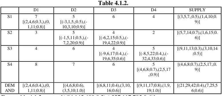
Stage II

We take & = [(3,5,7,;0.5),(1,4,10;0.9)], * = [(5,7,14;0.7),(1,6,15;0.9)]

₊= [(9,11,13;0.3),(3,10,14;0.5)], _, = [(4,6,8;0.7),(2,5,17,;0.9)] ,

'& = [(2,4,6;0.3,),(0,1,11;0.8)] , '* = [(4,6,8;0.6), (3,5,10;1.0)],

'₊ = [(6,8,11;0.4),(3,10,16;0.6)], '_, = [(9,11,17;0.8),(1,9,19;1.0)] .

Table 4.1.2.

D1 D2 D3 D4 SUPPLY

S1 7

[(2,4,6;0.3,),(0, 1,11;0.8)]

5

[(-3,1,5,;0.5),(-10,3,10;0.9)]

6 4 [(3,5,7,;0.5),(1,4,10;0. 9)]

S2 3 5

[(-1,5,11;0.5,),(-7,2,20;0.9)]

4

[(-6,2,15;0.5,),(-19,4,22;0.9)]

2 [(5,7,14;0.7),(1,6,15;0. 6)]

S3 4 6 4

[(-9,6,17;0.4,),(-19,6,35;0.6)]

5

[(-8,5,22;0.4,),(-32,4,33;0.6)]

[(9,11,13;0.3),(3,10,14 ;0.5)]

S4 8 7 6 5

[(4,6,8;0.7),(2,5,17 ,;0.9)]

[(4,6,8;0.7),(2,5,17,;0. 9)]

DEM AND

[(2,4,6;0.4,),(0, 1,11;0.8)]

[(4,6,8;0.6), (3,5,10;1.0)]

[(6,8,11;0.4),(3,10, 16;0.6)]

[(9,11,17;0.8),(1,9, 19;1.0)]

[(21,29,42;0.4),(7,25,5 6;0.6)] From table 4.1.2 we get [(-86,145,400;0.3),(-327,117,705;0.6)]

Therefore the optimal value of the objective function of the problem is given by minimum ={Stage I+ Stage II} = [(-172,290,800;0.3),(-654,234,1410;0.6)] =318.

4.2. North east corner rule Stage I

We take & = [(3,5,7,;0.5),(1,4,10;0.9)], * = [(5,7,14;0.7),(1,6,15;0.9)]

₊= [(9,11,13;0.3),(3,10,14;0.5)], _, = [(4,6,8;0.7),(2,5,17,;0.9)] ,

'& = [(2,4,6;0.3,),(0,1,11;0.8)] , '* = [(4,6,8;0.6), (3,5,10;1.0)],

(6)

82 Table 4.2.1.

D1 D2 D3 D4 SUPPLY

S1 7

[(2,4,6;0.3,),(0, 1,11;0.8)]

5

[(-16,1,18;0.5),(-39,3,39;0.9)]

6 4 [(3,5,7,;0.5),(1,4,10;0. 9)]

S2 3 5

[(-10,5,20;0.5,),(-29,2,42;0.9)]

4

[(-6,2,15;0.5,),(-27,4,30;0.9)]

2 [(5,7,14;0.7),(1,6,15;0. 9)]

S3 4 6 4

[(-4,6,12;0.4,),(-14,6,30;0.6)]

5

[(1,5,13;0.4,),(-16,4,17;0.6)]

[(9,11,13;0.3),(3,10,14 ;0.6)]

S4 8 7 6 5

[(4,6,8;0.7),(2,5,17 ,;0.9)]

[(4,6,8;0.7),(2,5,17,;0. 9)]

DEM AND

[(2,4,6;0.3,),(0, 1,11;0.8)]

[(4,6,8;0.6), (3,5,10;1.0)]

[(6,8,11;0.4),(3,10, 16;0.6)]

[(9,11,17;0.8),(1,9, 19;1.0)]

[(21,29,42;0.4),(7,25,5 6;0.6)]

From table 4.2.1 we get [(-131,145,445;0.3),(-574,117,892;0.6)] Stage II

We take _& = [(3,5,7,;0.5),(1,4,10;0.9)], _* = [(5,7,14;0.7),(1,6,15;0.9)]

+= [(9,11,13;0.3),(3,10,14;0.5)], , = [(4,6,8;0.7),(2,5,17,;0.9)] ,

'& = [(2,4,6;0.3,),(0,1,11;0.8)] , '* = [(4,6,8;0.6), (3,5,10;1.0)],

'+ = [(6,8,11;0.4),(3,10,16;0.6)], ', = [(9,11,17;0.8),(1,9,19;1.0)] .

Table 4.2.2.

D1 D2 D3 D4 SUPPLY

S1 7

[(2,4,6;0.3,),(0, 1,11;0.8)]

5

[(-16,1,18;0.5),(-39,3,39;0.9)]

6 4 [(3,5,7,;0.5),(1,4,10;0. 9)]

S2 3 5

[(-10,5,20;0.5,),(-29,2,42;0.9)]

4

[(-6,2,15;0.5,),(-27,4,30;0.9)]

2 [(5,7,14;0.7),(1,6,15;0. 9)]

S3 4 6 4

[(-4,6,12;0.4,),(-14,6,30;0.6)]

5

[(1,5,13;0.4,),(-16,4,17;0.6)]

[(9,11,13;0.3),(3,10,14 ;0.6)]

S4 8 7 6 5

[(4,6,8;0.7),(2,5,17 ,;0.9)]

[(4,6,8;0.7),(2,5,17,;0. 9)]

DEM AND

[(2,4,6;0.3,),(0, 1,11;0.8)]

[(4,6,8;0.6), (3,5,10;1.0)]

[(6,8,11;0.4),(3,10, 16;0.6)]

[(9,11,17;0.8),(1,9, 19;1.0)]

[(21,29,42;0.3),(7,25,5 6;0.6)]

From table 4.2.2 we get [(-131,145,445;0.3),(-574,117,892;0.6)]

Therefore the optimal value of the objective function of the problem is given by minimum ={Stage I+ Stage II} = [(-262,290,890;0.3),(-1148,234,1784;0.6)] =298

4.3. Least cost method Stage I

We take & = [(3,5,7,;0.5),(1,4,10;0.9)], * = [(5,7,14;0.7),(1,6,15;0.9)]

₊= [(9,11,13;0.3),(3,10,14;0.5)], _, = [(4,6,8;0.7),(2,5,17,;0.9)] ,

(7)

83

'₊ = [(6,8,11;0.4),(3,10,16;0.6)], '_, = [(9,11,17;0.8),(1,9,19;1.0)] .

Table 4.3.1.

D1 D2 D3 D4 SUPPLY

S1 7 5

[(-9,1,12;0.3,),(-17,1,24;0.6)]

6 4

[(-5,4,12;0.3,),(-14,3,18;0.6)]

[(3,5,7,;0.5),(1,4,10;0. 9)]

S2 3 5 4 2

[(5,7,14;0.7),(1,6,1 5;0.9)]

[(5,7,14;0.7),(1,6,15;0. 9)]

S3 4

[(2,4,6;0.3,),(0, 1,11;0.8)]

6 4

[(3,7,11;0.3,),(-8,9,14;0.6)]

5 [(9,11,13;0.3),(3,10,14 ;0.6)]

S4 8 7

[(-8,5,17;0.3,),(-21,4,27;0.6)]

6

[(-5,1,8;0.3,),(-11,1,24;0.6)]

5 [(4,6,8;0.7),(2,5,17,;0. 9)]

DEM AND

[(2,4,6;0.3,),(0, 1,11;0.8)]

[(4,6,8;0.6), (3,5,10;1.0)]

[(6,8,11;0.4),(3,10, 16;0.6)]

[(9,11,17;0.8),(1,9, 19;1.0)]

[(21,29,42;0.3),(7,25,5 6;0.6)]

From table 4.3.1 we get [(-121,12,371;0.3),(-384,103,655;0.6)]

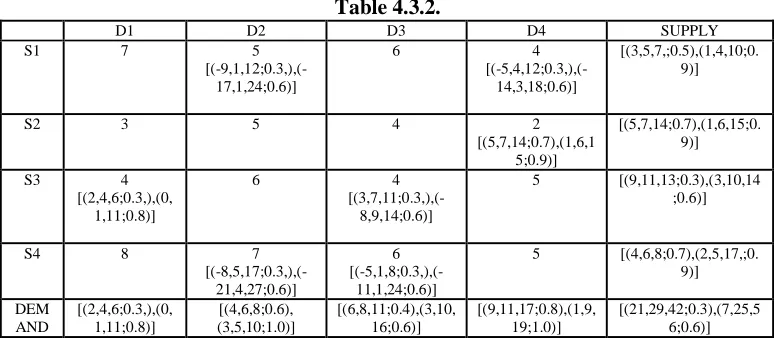
Stage II

We take _& = [(3,5,7,;0.5),(1,4,10;0.9)], _* = [(5,7,14;0.7),(1,6,15;0.9)]

+= [(9,11,13;0.3),(3,10,14;0.5)], , = [(4,6,8;0.7),(2,5,17,;0.9)] ,

'& = [(2,4,6;0.3,),(0,1,11;0.8)] , '* = [(4,6,8;0.6), (3,5,10;1.0)],

'₊ = [(6,8,11;0.4),(3,10,16;0.6)], '_, = [(9,11,17;0.8),(1,9,19;1.0)] .

Table 4.3.2.

D1 D2 D3 D4 SUPPLY

S1 7 5

[(-9,1,12;0.3,),(-17,1,24;0.6)]

6 4

[(-5,4,12;0.3,),(-14,3,18;0.6)]

[(3,5,7,;0.5),(1,4,10;0. 9)]

S2 3 5 4 2

[(5,7,14;0.7),(1,6,1 5;0.9)]

[(5,7,14;0.7),(1,6,15;0. 9)]

S3 4

[(2,4,6;0.3,),(0, 1,11;0.8)]

6 4

[(3,7,11;0.3,),(-8,9,14;0.6)]

5 [(9,11,13;0.3),(3,10,14 ;0.6)]

S4 8 7

[(-8,5,17;0.3,),(-21,4,27;0.6)]

6

[(-5,1,8;0.3,),(-11,1,24;0.6)]

5 [(4,6,8;0.7),(2,5,17,;0. 9)]

DEM AND

[(2,4,6;0.3,),(0, 1,11;0.8)]

[(4,6,8;0.6), (3,5,10;1.0)]

[(6,8,11;0.4),(3,10, 16;0.6)]

[(9,11,17;0.8),(1,9, 19;1.0)]

[(21,29,42;0.3),(7,25,5 6;0.6)]

From table 4.3.2 we get [(-121,12,371;0.3),(-384,103,655;0.6)] .

(8)

84 4.4. Vogel’s approximation method

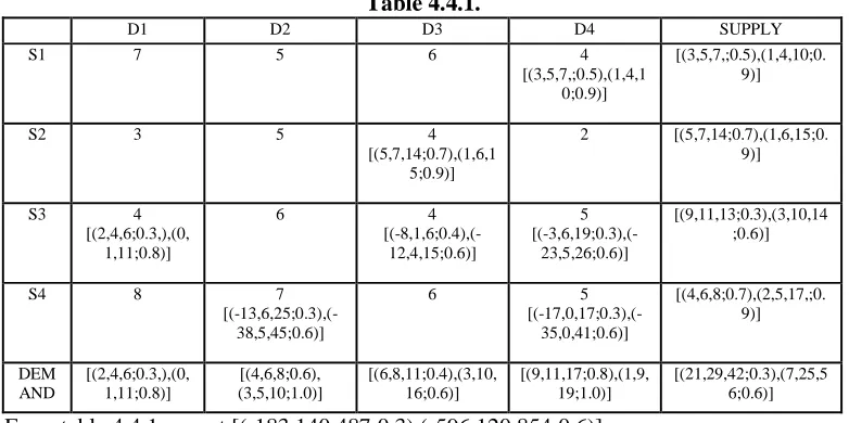
Stage I

We take & = [(3,5,7,;0.5),(1,4,10;0.9)], * = [(5,7,14;0.7),(1,6,15;0.9)]

₊= [(9,11,13;0.3),(3,10,14;0.5)], _, = [(4,6,8;0.7),(2,5,17,;0.9)] ,

'& = [(2,4,6;0.3,),(0,1,11;0.8)] , '* = [(4,6,8;0.6), (3,5,10;1.0)],

'₊ = [(6,8,11;0.4),(3,10,16;0.6)], '_, = [(9,11,17;0.8),(1,9,19;1.0)] .

Table 4.4.1.

D1 D2 D3 D4 SUPPLY

S1 7 5 6 4

[(3,5,7,;0.5),(1,4,1 0;0.9)]

[(3,5,7,;0.5),(1,4,10;0. 9)]

S2 3 5 4

[(5,7,14;0.7),(1,6,1 5;0.9)]

2 [(5,7,14;0.7),(1,6,15;0. 9)]

S3 4

[(2,4,6;0.3,),(0, 1,11;0.8)]

6 4

[(-8,1,6;0.4),(-12,4,15;0.6)]

5

[(-3,6,19;0.3),(-23,5,26;0.6)]

[(9,11,13;0.3),(3,10,14 ;0.6)]

S4 8 7

[(-13,6,25;0.3),(-38,5,45;0.6)]

6 5

[(-17,0,17;0.3),(-35,0,41;0.6)]

[(4,6,8;0.7),(2,5,17,;0. 9)]

DEM AND

[(2,4,6;0.3,),(0, 1,11;0.8)]

[(4,6,8;0.6), (3,5,10;1.0)]

[(6,8,11;0.4),(3,10, 16;0.6)]

[(9,11,17;0.8),(1,9, 19;1.0)]

[(21,29,42;0.3),(7,25,5 6;0.6)]

From table 4.4.1 we get [(-183,140,487;0.3),(-596,120,854;0.6)] Stage II

We take & = [(3,5,7,;0.5),(1,4,10;0.9)], * = [(5,7,14;0.7),(1,6,15;0.9)]

+= [(9,11,13;0.3),(3,10,14;0.5)], , = [(4,6,8;0.7),(2,5,17,;0.9)] ,

'& = [(2,4,6;0.3,),(0,1,11;0.8)] , '* = [(4,6,8;0.6), (3,5,10;1.0)],

'+ = [(6,8,11;0.4),(3,10,16;0.6)], ', = [(9,11,17;0.8),(1,9,19;1.0)] .

Table 4.4.2.

D1 D2 D3 D4 SUPPLY

S1 7 5 6 4

[(3,5,7,;0.5),(1,4,1 0;0.9)]

[(3,5,7,;0.5),(1,4,10;0. 9)]

S2 3 5 4

[(5,7,14;0.7),(1,6,1 5;0.9)]

2 [(5,7,14;0.7),(1,6,15;0. 9)]

S3 4

[(2,4,6;0.3,),(0, 1,11;0.8)]

6 4

[(-8,1,6;0.4),(-12,4,15;0.6)]

5

[(-3,6,19;0.3),(-23,5,26;0.6)]

[(9,11,13;0.3),(3,10,14 ;0.6)]

S4 8 7

[(-13,6,25;0.3),(-38,5,45;0.6)]

6 5

[(-17,0,17;0.3),(-35,0,41;0.6)]

[(4,6,8;0.7),(2,5,17,;0. 9)]

DEM AND

[(2,4,6;0.3,),(0, 1,11;0.8)]

[(4,6,8;0.6), (3,5,10;1.0)]

[(6,8,11;0.4),(3,10, 16;0.6)]

[(9,11,17;0.8),(1,9, 19;1.0)]

(9)

85

From table 4.4.2 we get [(-183,140,487;0.3),(-596,120,854;0.6)]

Therefore the optimal value of the objective function of the problem is given by minimum = {Stage I+ Stage II} = [(-366,280,974;0.3),(-1192,240,1708;0.6)] =274.

4.5. U-V distribution method Stage I

We take & = [(3,5,7,;0.5),(1,4,10;0.9)], * = [(5,7,14;0.7),(1,6,15;0.9)]

+= [(9,11,13;0.3),(3,10,14;0.5)], , = [(4,6,8;0.7),(2,5,17,;0.9)] ,

'& = [(2,4,6;0.3,),(0,1,11;0.8)] , '* = [(4,6,8;0.6), (3,5,10;1.0)],

'₊ = [(6,8,11;0.4),(3,10,16;0.6)], '_, = [(9,11,17;0.8),(1,9,19;1.0)] .

Table 4.5.1.

D1 D2 D3 D4 SUPPLY

S1 7 5

[(3,5,7,;0.5),(1,4,1 0;0.9)]

6 4 [(3,5,7,;0.5),(1,4,10;0. 9)]

S2 3 5 4 2

[(5,7,14;0.7),(1,6,1 5;0.9)]

[(5,7,14;0.7),(1,6,15;0. 9)]

S3 4

[(2,4,6;0.3,),(0, 1,11;0.8)]

6 4

[(3,7,11;0.3),(-8,9,14;0.6)]

5 [(9,11,13;0.3),(3,10,14 ;0.6)]

S4 8 7

[(-3,1,5,;0.5),(-7,1,9;0.9)]

6

[(-5,1,8;0.3),(-11,1,24;0.6)]

5

[(-5,4,12;0.3),(-14,3,18;0.6)]

[(4,6,8;0.7),(2,5,17,;0. 9)]

DEM AND

[(2,4,6;0.3,),(0, 1,11;0.8)]

[(4,6,8;0.6), (3,5,10;1.0)]

[(6,8,11;0.4),(3,10, 16;0.6)]

[(9,11,17;0.8),(1,9, 19;1.0)]

[(21,29,42;0.3),(7,25,5 6;0.6)]

From table 4.5.1 we get [(-31,116,274;0.3),(-210,100,477;0.6)]

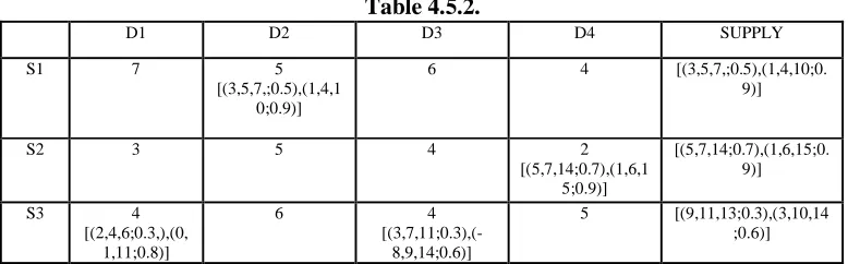
Stage II

We take _& = [(3,5,7,;0.5),(1,4,10;0.9)], _* = [(5,7,14;0.7),(1,6,15;0.9)]

+= [(9,11,13;0.3),(3,10,14;0.5)], , = [(4,6,8;0.7),(2,5,17,;0.9)] ,

'_& = [(2,4,6;0.3,),(0,1,11;0.8)] , '_* = [(4,6,8;0.6), (3,5,10;1.0)],

'+ = [(6,8,11;0.4),(3,10,16;0.6)], ', = [(9,11,17;0.8),(1,9,19;1.0)] .

Table 4.5.2.

D1 D2 D3 D4 SUPPLY

S1 7 5

[(3,5,7,;0.5),(1,4,1 0;0.9)]

6 4 [(3,5,7,;0.5),(1,4,10;0. 9)]

S2 3 5 4 2

[(5,7,14;0.7),(1,6,1 5;0.9)]

[(5,7,14;0.7),(1,6,15;0. 9)]

S3 4

[(2,4,6;0.3,),(0, 1,11;0.8)]

6 4

[(3,7,11;0.3),(-8,9,14;0.6)]

(10)

86

S4 8 7

[(-3,1,5,;0.5),(-7,1,9;0.9)]

6

[(-5,1,8;0.3),(-11,1,24;0.6)]

5

[(-5,4,12;0.3),(-14,3,18;0.6)]

[(4,6,8;0.7),(2,5,17,;0. 9)]

DEM AND

[(2,4,6;0.3,),(0, 1,11;0.8)]

[(4,6,8;0.6), (3,5,10;1.0)]

[(6,8,11;0.4),(3,10, 16;0.6)]

[(9,11,17;0.8),(1,9, 19;1.0)]

[(21,29,42;0.3),(7,25,5 6;0.6)]

From table 4.5.2 we get [(-31,116,274;0.3),(-210,100,477;0.6)].

Therefore the optimal value of the objective function of the problem is given by minimum ={Stage I+ Stage II} = [(-62,232,548;0.3),(-420,200,954;0.6)] =242.

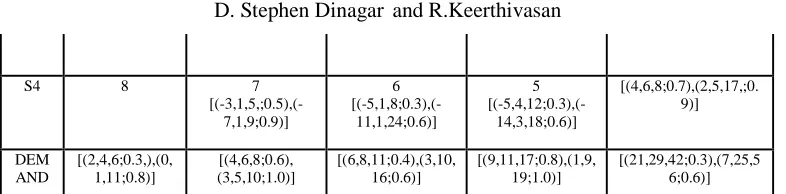
4.6. Best candidate method Stage I

We take _& = [(3,5,7,;0.5),(1,4,10;0.9)], _* = [(5,7,14;0.7),(1,6,15;0.9)]

+= [(9,11,13;0.3),(3,10,14;0.5)], , = [(4,6,8;0.7),(2,5,17,;0.9)] ,

'_& = [(2,4,6;0.3,),(0,1,11;0.8)] , '_* = [(4,6,8;0.6), (3,5,10;1.0)],

'+ = [(6,8,11;0.4),(3,10,16;0.6)], ', = [(9,11,17;0.8),(1,9,19;1.0)] .

Table 4.6.1.

D1 D2 D3 D4 SUPPLY

S1 7 5

[(3,5,7,;0.5),(1,4,1 0;0.9)]

6 4 [(3,5,7,;0.5),(1,4,10;0. 9)]

S2 3 5 4 2

[(5,7,14;0.7),(1,6,1 5;0.9)]

[(5,7,14;0.7),(1,6,15;0. 9)]

S3 4

[(2,4,6;0.3,),(0, 1,11;0.8)]

6 4

[(3,7,11;0.3),(-8,9,14;0.6)]

5 [(9,11,13;0.3),(3,10,14 ;0.6)]

S4 8 7

[(-16,1,18;0.3),(-40,1,42;0.6)]

6

[(-5,1,8;0.3),(-11,1,24;0.6)]

5

[(-5,4,12;0.7),(-14,3,18;0.9)]

[(4,6,8;0.7),(2,5,17,;0. 9)]

DEM AND

[(2,4,6;0.3,),(0, 1,11;0.8)]

[(4,6,8;0.6), (3,5,10;1.0)]

[(6,8,11;0.4),(3,10, 16;0.6)]

[(9,11,17;0.8),(1,9, 19;1.0)]

[(21,29,42;0.3),(7,25,5 6;0.6)] From table 4.6.1 we get [(-122,116,365;0.3),(-441,100,708;0.6)].

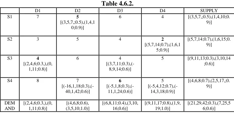
Stage II

We take _& = [(3,5,7,;0.5),(1,4,10;0.9)], _* = [(5,7,14;0.7),(1,6,15;0.9)]

+= [(9,11,13;0.3),(3,10,14;0.5)], , = [(4,6,8;0.7),(2,5,17,;0.9)] ,

'_& = [(2,4,6;0.3,),(0,1,11;0.8)] , '_* = [(4,6,8;0.6), (3,5,10;1.0)],

(11)

87 Table 4.6.2.

D1 D2 D3 D4 SUPPLY

S1 7 5

[(3,5,7,;0.5),(1,4,1 0;0.9)]

6 4 [(3,5,7,;0.5),(1,4,10;0. 9)]

S2 3 5 4 2

[(5,7,14;0.7),(1,6,1 5;0.9)]

[(5,7,14;0.7),(1,6,15;0. 9)]

S3 4

[(2,4,6;0.3,),(0, 1,11;0.8)]

6 4

[(3,7,11;0.3),(-8,9,14;0.6)]

5 [(9,11,13;0.3),(3,10,14 ;0.6)]

S4 8 7

[(-16,1,18;0.3),(-40,1,42;0.6)]

6

[(-5,1,8;0.3),(-11,1,24;0.6)]

5

[(-5,4,12;0.7),(-14,3,18;0.9)]

[(4,6,8;0.7),(2,5,17,;0. 9)]

DEM AND

[(2,4,6;0.3,),(0, 1,11;0.8)]

[(4,6,8;0.6), (3,5,10;1.0)]

[(6,8,11;0.4),(3,10, 16;0.6)]

[(9,11,17;0.8),(1,9, 19;1.0)]

[(21,29,42;0.3),(7,25,5 6;0.6)]

From table 4.6.2 we get [(-122,116,365;0.3),(-441,100,708;0.6)]

Therefore the optimal value of the objective function of the problem is given by minimum={Stage I+ Stage II} = [(-244,232,730;0.3),(-882,200,1416;0.6)] =242.

5. Result and discussion

For the given example here, initial basic feasible solution obtained by

North- West Corner Rule gives Ɍ [(-172,290,800;0.3),(-654,234,1410;0.6)] =318. North -East Corner Rule gives Ɍ [(-262,290,890;0.3),(-1148,234,1784;0.6)] =298. Least Cost method gives Ɍ [(-242,240,742;0.3),(-762,206,1310;0.6)] =249.

Vogel’s Approximation Method gives Ɍ [(-366,280,974;0.3),(-1192,240,1708;0.6)] =274. U-V Distribution Method gives Ɍ [(-62,232,548;0.3),(-420,200,954;0.6)] =242.

Best Candidate Method gives Ɍ [(-244,232,730;0.3),(-882,200,1416;0.6)] =242.

6. Conclusion

For most of the fuzzy transportation problems, the initial basic feasible solution obtained by Best Candidate Method is an optimal solution .For some fuzzy Transportation problems, the initial basic feasible solution obtained by Vogel’s Approximation Method is optimal ,but it is not optimal for some other problems. On the other hand North West Corner Rule, North East Corner Rule, Least Cost method usually gives the optimal. Therefore, Best Candidate Method is preferred comparison to the other methods for finding the initial basic feasible solution of the Fuzzy Transportation Problem.

REFERENCES

1. A.Nagoorgani and K.Abdul Razak, Two stage fuzzy transportation problem, Journal

of Physical Sciences, 10 (2006) 63-69.

(12)

88

3. D.Stephen Dinagar and R.Keerthivasan, On fuzzy transportation problems with the best candidate method, Annals Pure and Applied Mathematics, 13(2) (2017) 382-388. 4. L.Zadeh and R.Bellman, Decision making in a fuzzy environment, Management

Science,17(1970) 141-164.

5. Omar M.Saad and Shamir A.Abbas, A parametric study on transportation problem under fuzzy Environment, The Journal of Fuzzy Mathematics, 11(11) (2003)115-124.

6. S.Chanas, W.Kolodziejczyk and A.Machaj, A fuzzy approach to the transportation problem, Fuzzy Sets and Systems, (1984) 211-221.