Notes on the Power Sum $1^k+2^k+...+n^k$

(1)

Vol. 9, No. 2, 2015, 215-232

ISSN: 2279-087X (P), 2279-0888(online) Published on 25 March 2015

www.researchmathsci.org

215

Notes on the Power Sum 1

k

+2

k

+...+n

k

Moawwad El-Mikkawy and Faiz Atlan

Mathematics Department, Faculty of Science, Mansoura University, Mansoura-35516, Egypt

E-mails: m_elmikkawy@yahoo.com, faizatlan11@yahoo.com

Received 9 February 2015; accepted 3 March 2015

Abstract. In this paper we present some efficient computational methods to compute the power sum ( )= ,

1 =

k n

r k n r

S

∑

for integers k≥0, and n≥1. A new method to compute )

(n

S_k is investigated. Some new identities involving S_k(n) are given.

Keywords: Power sum; Bernoulli numbers; Vandermonde matrix; Stirling numbers; Eulerian numbers; Linear systems; Elementary symmetric polynomials; Exponential generating function

AMS Mathematics Subject Classification (2010): 65F05, 68W30, 15Bxx, 11B73, 05E05

1. Introduction and basic definitions

One of the oldest topics in mathematics is the summation of powers ,

... 2 1 = =

) (

1 =

k k

k k n

r

k n r n

S

∑

+ + + (1) for integers k≥0, and n≥1. The interested reader may refer to [1, 2, 4, 5, 7, 8, 12, 13, 14, 15, 16, 19, 22, 23, 24, 29, 31, 32, 33, 35, 38, 40, 42, 43, 44] for the history of this problem. Even nowadays there is a continual stream of publications on the topic. See for instance, [6, 10, 11, 20, 21, 26, 27, 28, 34, 36, 39, 41] and the references therein. Throughout this paper,

δ

_ij is the kronecker delta which is equal to 1 or 0 according as

j

i = or not. Also [xr]P(x),

denotes the coefficients of xr in the polynomial P(x), and empty summation is assumed equal to zero.

Definition 1.1. [34] The exponential generating function (EGF) of a sequence

> ,... , ,

<a₀ a₁ a₂ is defined by:

. ! =

) (

0

= n

x a x

f

n n n

∑

∞

(2)

216

0. ,

= ,

! =

!

! =0 =0 =0

0 =

≥ 

     

  

     

 

− ∞

∞ ∞

∑

a b n

k n c

where n

x c n

x b n x

a k n k

n

k n n

n n n n n n n

n

(2)

The EGF, G(n,x) of Sk(n) is given by: .

! ) ( = 1

1 =

) , (

0

= i

x n S e

e x n G

i i i x nx

∑

∞

− −

−

(3) Definition 1.2. [37] For integer numbers n and k with n≥k≥0, the Stirling numbers of the first kind, s(n,k) and of the second kind, S(n,k) are defined respectively by:

, ) , ( = 1] [

= ) (

0 =

k n

n x n s n k x

x − +

∑

(4) and

, ) ( ) , ( =

0 =

k n

x k n S

x

∑

(5) where the falling factorial of x, (x)_n and the rising factorial of x, [x]_n are given respectively by:

  

≥ +

− −

−1)( 2)...( 1) 1,

(

, 0 = 1

= ) (

n if n

x x

n if x _n

(6) and

  

≥ −

+ +

+1)( 2)...( 1) 1.

(

, 0 = 1

= ] [

n if n

x x

n if x _n

(7) It is well known that for integers n,k≥0, s(n,k) and S(n,k) satisfy the following Pascal-type recurrence relations:

), 1, ( 1) ( 1) 1, ( = ) ,

(n k s n k n s n k

s − − − − − (8) and

), 1, ( 1) 1, ( = ) ,

(n k S n k kS n k

S − − + − (9) subject to:

n k k

k S k k

s( , )= ( , )=1,1≤ ≤ (10) and

0. = 0 = , = ) , ( = ) ,

(n k S n k if k orn

s

δ

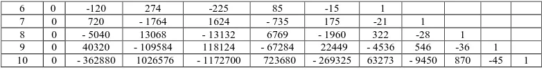
nk (11)

The values of the Stirling numbers of the first kind s(n,k) and of the second kind )

, (n k

S for 0≤n,k≤10 are the entries in the following tables:

n/k 0 1 2 3 4 5 6 7 8 9 10

0 1

1 0 1

2 0 -1 1

3 0 2 -3 1

4 0 -6 11 -6 1

(3)

217

6 0 -120 274 -225 85 -15 1 7 0 720 - 1764 1624 - 735 175 -21 1

8 0 - 5040 13068 - 13132 6769 - 1960 322 -28 1 9 0 40320 - 109584 118124 - 67284 22449 - 4536 546 -36 1 10 0 - 362880 1026576 - 1172700 723680 - 269325 63273 - 9450 870 -45 1

Table 1: The Stirling numbers of the first kind s(n,k) for 0≤n,k≤10.

n/k 0 1 2 3 4 5 6 7 8 9 10

0 1

1 0 1

2 0 1 1

3 0 1 3 1

4 0 1 7 6 1

5 0 1 15 25 10 1

6 0 1 31 90 65 15 1

7 0 1 63 301 350 140 21 1

8 0 1 127 966 1701 1050 266 28 1 9 0 1 255 3035 7770 6951 2646 462 36 1 10 0 1 511 9330 34501 42525 22827 5880 750 45 1

Table 2: The Stirling numbers of the second kind S(n,k) for 0≤n,k≤10.

Definition 1.3. [20] The Bernoulli numbers, B_i,i≥0 and polynomials, B_i(x),i≥0 are defined by:

1, , 1 1

1 = 1, =

1

0 =

0 ≥

  

 

  

  +

+

−

∑

− j B i i

i B

B _j

i

j

i (12)

and

0 , =

) (

0 =

≥ 

 

 

  

 

−

∑

j B x i

i

x

B i j j

i

j

i (13)

respectively.

The exponential generating functions of the Bernoulli numbers, B_i,i≥0 and polynomials, B_i(x),i≥0 are given by:

. ! =

1 = ) (

0

= n

t B e

t t H

n n n t

∑

∞

− (14) and

, ! ) ( = 1 = ) , (

0

= n

t x B e

te t x F

n n n t

x t

∑

∞

− (15) respectively.

(4)

218 include [18, 37]:

1. 0,

> 1)

(− 1 ₂ ≥

• +

k B_k

k

(16) • B₂_k₊₁=0, k≥1. (17)

0. ,

= 1

1

0 =

≥ 

 

 

  

 

•

∑

− k B n n

n k n

k

δ

(18)

• Bi(x+1)−Bi(x)=ixi−1, i≥1. (19) The first few Bernoulli numbers B_n, and Bernoulli polynomials B_n(x) are given, respectively, in the following tables:

n

0 1 2 3 4 5 6 7 8 9 10 11 12 13 14

n

B 1

2 1 −

6 1 0

30 1 − 0

42

1 0

30 1 − 0

66

5 0

2730 691

− 0

6 7 Table 3: The Bernoulli numbers B_n for 0≤n≤14.

n 0

1 2 3 4 5

) (x

B_n

1

2 1 −

x

6 1 2− +

x

x x x x

2 1 2 3 2

3− +

30 1 2 3 2

4− + −

x x

x x x x x

6 1 3 5 2

5 4 3

5− + −

Table 4: The Bernoulli polynomials Bn(x) for 0≤n≤5.

Definition 1.4. [37] For each n≥1, the Eulerian numbers E(n,k) are defined by:

1. 0

, ) 1 ( 1 1) ( = ) , (

0 =

− ≤ ≤ −

+   

 

  

  + −

∑

j k j k n

n k

n

E j n

k

j

(20)

The values of the Eulerian numbers E(n,k) for 1≤n≤10 and 0≤k≤9, are the entries in the following table

n/k 0 1 2 3 4 5 6 7 8 9

1 1 2 1 1

3 1 4 1

4 1 11 11 1

5 1 26 66 26 1

6 1 57 302 302 57 1

(5)

219

8 1 247 4293 15619 15619 4293 247 1

9 1 502 14608 88234 156190 88234 14608 502 1 10 1 1013 47840 455192 1310354 1310354 455192 47840 1013 1

Table 5: The Eulerian numbers E(n,k) for 1≤n≤10 and 0≤k≤9. The Eulerian numbers E(n,k) satisfy:

1. 1,

= 1) , ( = ,0)

( − ≥

•E n E n n n (21) 1.

), 1 , ( = ) ,

( − − ≥

•E n k E n n k n (22) 2.

1), 1, ( ) ( ) 1, ( 1) ( = ) ,

( + − + − − − ≥

•E n k k E n k n k E n k n (23)

Definition 1.5. [26] The elementary symmetric polynomial

σ

r(n) in x1,x2,…,xn is

defined by:

      

≤ ≤

∑

≤ ≤

. 1

0, = 1

0), < ( ) > ( 0

= ) , , , (

2 1 < < 2 < 1 1 2

1 ) (

n r if x x x

r if

n or n r if x

x x

r i i i n r i i i n

n r

… …

…

σ

(24)

It should be noted that

σ

r(n) is a homogenous function and can be written as:

. , 0,1, = , =

) , , ,

( 2

2 1 1

{0,1} , , 2 , 1 = 2 1 2

1 ) (

n r

x x x x

x

x kn

n k k

n k k k r n k k k n n

r … … …

… …

∑

∈ +

+ +

σ

(25)

The symmetric polynomials

σ

_r( n) satisfies the recurrence relation: ). , , , ( )

, , , ( = ) , , ,

( 1 2 1

1) (

1 1

2 1 1) ( 2

1 ) (

− −

− ₊

n n

r n n n

r n n

r x x … x

σ

x x … x x

σ

x x … x

σ

(26)

A more general form of (26) is given by:

), , , , , , , ( )

, , , , , , ( = ) , , ,

( ₁ ₂ ( 1) ₁ ₂ ₁ ₁ (₁1) ₁ ₂ ₁ ₁

) (

n j j n

i j n j j n

i n n

i x x …x x x …x x …x x x x …x− x+ …x

− − +

−

− ₊

_σ

σ

(27)

where 1≤i, j≤n.

Partial differentiation for both sides of (27) with respect to xj gives:

∂∂x_j

σ

_i(n) =

σ

_i(_,n_j) =

σ

_i(₋n₁−1)(x₁,x₂,…,x_j₋₁,x_j₊₁,…,x_n).

(28) Therefore by using (24), we get:

  

   

 

≤ ≤ −

≠ − ≤ −

≤

∑

. 2

1, = 1

0), < ( ) > ( 0

= ) , , , (

1 2 1

1 , 2 , 1 1 < < 2 < 1 1 2

1 ) (

n i if x x x

i if

n or n i if x

x x

i r r r j i r r r n i r r r n

n ij

… …

σ

(29)

(6)

220

, 1

, ! = ) , 1, 1, , (1,2, ) (

, i n

i n n i

i

n i

n … − + … ≤ ≤

σ

(30)

and 2 , 1 .

1 = ) , 1, 1, , (1,2, ) (

2, i i n

n n i

i

n

i − ≤ ≤

  

 

  

  + +

− …

…

σ

(31)

Definition 1.6. [17] For the n+1 real values m,x₁,x₂,...,x_n we define a generalized Vandermonde matrix ( 1, 2,..., )

) (

n m

n x x x

V or simply V_n( m) by:

(

)

. =

1 = , 1 )

( n

j i i m j m n x

V +− (32) The values x1,x2,...,xn are called the nodes of the matrix .

) ( m

n

V The determinant of )

(m

n

V is given by:

). (

) ( = ) ( det

< 1 1 = ) (

j i n i j m r n

r m

n x x x

V

∏

−

≤ ≤

(33) Thus V_n( m) is invertible if and only if the n parameters x₁,x₂,...,x_n are distinct. Note that for any m, the two matrices Vn( m) and Vn =Vn

(0)

are related by: n

m n DV

V( ) =

(34) where = ( 1 , 2,..., ).

m n m m

x x x diag D

The explicit form of the inverse matrix, ij nij m

n

V( ) 1 _,₌₁ ) ( = )

( −

α

of the Vandermonde matrix V_n( m) is given by [17]:

. , 1 , ) (

) ,..., , ( 1)

( =

1 =

2 1 ) (

1,

n j i x

x x

x x x

r i n

i r r m i

n n

i j n j n

ij ≤ ≤

− −

∏

≠ + −

−

σ

α

(35)

Let (( ) ) =( ), =1, 1

)

( n

j i ij T

m n

V −

β

Then we have:

, , 1 , ) (

) ,..., , ( 1)

( =

1 =

2 1 ) (

1,

n j i x

x x

x x x

r j n

j r r m j

n n

j i n i n

ij ≤ ≤

− −

∏

≠ + −

−

σ

β

(36)

since the inverse of transpose is the transpose of the inverse. If xi =i for i=1,2,...,k+1, then (36) takes the form:

1. ,

1 1), (1,2,..., 1

1)! (

1) (

= ( 1)

,

2 + ≤ ≤ +

      ₊ +

− +

− + +

k j i k

j k

k

k j i k j

i

ij

σ

β

(37)

Definition 1.7. [20] The sequences <E0,E1,E2,...> of the Euler numbers, En,n≥0 is

(7)

221 .

! =

1 2

0 = 2

n x E e

e n

n n x

x

∑

∞

+ (38) In this paper, we are mainly interested in the power sum S_k(n)=1k +2k +...+nk for integers k≥0, and n≥1. We are also interested in the use of the generating function of

) (n

S_k to obtain new identities. In this framework, some computational methods for computing Sk(n) are given in Section 2. In Section 3, we investigate some new identities for Sk(n). In Section 4, we deal with a method for computing Sk(n) by solving a

special linear system of equations.

For the convenience of the reader we are going to list the following facts about )

(n

S_k [9, 26, 30, 40]: )

(n

Sk is a polynomial of degree k+1 in

n

without constant term. Hence

) (n

Sk takes the form:

( )= 1, , 0, 1

1 =

≥ +

+

∑

c n k

n

S k i i

k

i

k (39)

where the coefficients c_k₊_1,_i,i=1,2,...,k+1 are to be determined.

The sum of the coefficients of any polynomial Sk(n),k≥0 is always equals 1.

n

is a factor of S_k(n), k≥0.

n

and n+1 are factors of S_k(n), k≥1. ,

n n+1 and 2n+1 are factors of Sk(n), for even k≥2. 2

n (n+1)2 are factors of S_k(n), for odd k≥3. 0.

, 1 1 = =

) ( ] [ )

( 1, 1

1 ≥

+ + + +

k k

c n S n

g k k k

k

(40)

1. ,

2 1 = =

) ( ] [ )

(h n Sk n ck+1,k k≥

k

(41)

2. ,

12 = =

) ( ] [ )

( 1 _1, ₁ ≥

− + −

k k

c n S n

i k _k _k _k

(42) 3.

0, = =

) ( ] [ )

( 1, 2

2 ≥

− + −

k c

n S n

j k k k

k

(43) 4.

, 3 120

1 = =

) ( ] [ )

( 3 _1, ₃ _ ≥

     − − + −

k k

c n S n

k k _k _k _k

(44)

0. , 1) ( = =

= ) ( ] [ ) (

0 = 1,1

1 − ≥

     

∑

+ B B k

j k c

n S n

l k

k j

k

j k

k (45)

2. Some computational methods for computing Sk(n)

(8)

222 coefficients

  

 

  

 

q p

and the Bernoulli numbers, B_k which is given by:

0. ,

1 1)

( 1 1 = )

( 1

1 1

1 =

≥ 

 

 

  

  + −

+ +− +−

+

∑

j B n k

k

k n

S k j j

j k k

j k

(46)

From (39) and (46), we see that the coefficients ck+1,j are given by:

1. 1

, 1)

( 1 1

= 1 ₁

1, ₊ − ≤ ≤ +

      +

− + − +

+ B j k

k j k

c_k _j k j _k _j

(47) Formula (46) can also be written in the form:

. 1 1)

( = ) (

1

0

= +

     

− − − +

∑

j n B j k n

S

j j k j k k

j

k (48)

From (46)-(48), we see that:

. 1 1)

( = ) ( 1)

( = ) (

1

, 1 = 1

0 − + +

+

−

∫

−

∑

+

j n c k n B dx

x S k n B n

S

j j k k

j k k k

n k k k

(49) The formula (49) reveals that we can obtain S_k(n) from S_k₋₁(n) recursively for k≥1 with the initial condition S0(n)=n. For example, we have:

. 2 1 2 1 = )

( 2

1 n n n

S + .

3 1 2 1 6 1 = ) 3 2 1 2 2 1 2( 6 1 = )

( 2 3 2 3

2 n n n n n n n

S + + + +

, 4 1 2 1 4 1 = ) 4 3 1 3 2 1 2 6 1 3( 0. = )

( 2 3 4 2 3 4

3 n n n n n n n n

S + + + + +

having used Table 3 and (49).

There are many other ways to express the power sum Sk(n). See for instance [3, 25, 34]

, 1) ( 1

) , ( 1) ( =

)

( ₁

1 =

0+ +

∑

₊ − j−

k

j k

k n

j j k S n

n n n

S

δ

(50)

(

)

, (1) 1)

( 1 1 = )

( +1 + − +1

+ k k

k B n B

k n S

(51)

0. ,

1 1 )

, ( = )

( 0

1

0 =

≥ −

  

 

  

 

+ + +

∑

− k k

m n m k E n

S k

k

m

k

δ

(9)

223

0. ),

, (

) 1 1, ( ) ( =

) (

1) , (

0 =

≥ −

+ −

+ + −

∑

− n m s n n m S n k m n k

n S

n k min

m

k (53)

and S_k(n)=XQY,

(54) where

], 1 ... 2 1 [ =

  

 

  

 

+   

 

  

 

  

 

  

 

k n n

n

X 1 ],1=1

1 1)

[(

= − +

  

 

  

 

− −

− k

j i j

i

j i

Q and

. ] 1) ...( 2 [1

= k k k k T

Y +

An easy proof for (47) can be found in [30]. Also a very easy proof for the formula (51) can be obtained by using the property:

). (1, ) 1, ( = ) ,

(n x F n x F x

G

x + − (55) By using the property (19) together with the telescoping sum, an additional proof for the formula (51) can be obtained.

3. New identities for S_k(n)

The main objective of this section is to introduce new identities involving the power sum, ).

(n

Sk

By noticing that the coefficients ck+1,1,ck+1,2,...,ck+1,k+1 in (39) satisfy the Vandermonde linear system:

, 1) (

(3) (2) (1)

= 1)

( 1)

( 1) ( 1) (

3 3

2 2

1 1

1 1,

1,3 1,2 1,1

1 3

2

1 3

2

1 3

2

1 3

2

       

 

       

 

+ 

      

 

       

 

       

 

       

 

+ +

+

+ + +

+ + + +

k S

S S S

c c c c

k k

k

k k

k k k

k k

k k k

k k k k

⋮ ⋮

… ⋮ ⋮ ⋮

⋮

… … …

(56)

then following [17], together with (37) we obtain the coefficients ck₊_1,1,ck₊_1,2,...,ck₊_1,k₊₁

as follows:

1. 1

), ( 1

1)! (

1) (

= ( 21),

1

1 =

1,  ≤ ≤ +

     + +

− +

− + +

+

∑

S j i k

j k k

c k

k j i k j

i k

j i

k

σ

(57) We are now ready to formulate the following result.

Theorem 3.1. The power sum S_k(n) enjoys the following identities: 0.

, ! 1) ( = ) ( 1 1)

( )

( 1

1

1 =

≥ −

      + − + +

∑

S j k k

j k

i k

k j

k

j

(10)

224

1. ,

! 1) ( = ) ( ] 2 1 [ 1) ( ) (

1

1 =

≥ −

      +       ₊ −

∑

+ S j k k

j k

j k k

ii j _k k

k

j

(59)

0. ,

1) ( = ) ( 1 1)

( )

( 1

1

1 =

≥ −

      +

− + +

∑

S j B k

j j k

iii k

k k

j k

j

(60)

0. ,

= ) ( 1)

( )

( 0

1 1

0 =

≥ −

      − +− −

∑

S n n i

j i

iv i

i j

j i i

j

δ

(61)

0. ,

) ( = 1) ( )

( 1 =

≥ − −

     

∑

S n S n n i

j i

v _j _i

i

j

(62)

0. ),

( 2 ) (2 = ) ( )

(

1

0 =

≥ −

      − −

∑

S n S n S n i

j i n

vi j i i

j i i

j

(63)

0. 1),

( =

) ( 1)

( )

( ₀

0 =

≥ −

+ 

     − −

∑

S n S n i

j i

vii i j _j _i _i

i

j

δ

(64)

    

≥ −

−       − − −

∑

. 0

1, ,

1) ( 2 =

1) ( 1)

( ) (

1

0 =

even is i if

i odd is i if n

S n

S j i n viii

i j

j i j i

j

(65)

0. ,

1) ( 1) ( = ) ( )

( )

( 0

0 =

≥ +

− −

      − −

∑

S n S n i

j i n

ix i i

i j

j i i

j

δ

(66)

Proof: (i) Putting i=k+1 in (57) together with (40) gives:

), ( 1)! (

1 1)

( = ) ( 1)!

( 1 1)

( = 1

1 1

1

1 = 1)

( 1, 1

1

1 =

j S k

j k

j S k

j k

k k

j k k

j j

k k

j +

      +

− +

      +

− +

+ + + +

+ + +

∑

σ

(67)

having used (29). Therefore

0, ,

! 1) ( = ) ( 1 1)

( 1

1

1 =

≥ −

      + − + +

∑

S j k k

j

k _k

k j

k

j

on simplification.

(11)

225 ), ( 1)! ( 1 ] 2 2 [ 1) ( = ) ( 1)! ( 1 1) ( = 2 1 1 1 = 1) ( 2, 1 1 = j S k j k j k j S k j k k j k k j k k j j k k j +       ₊ −       ₊ − +       ₊ − + + + + +

∑

σ

(68)

having used (31). Then

1. ), ( 1 1) ( 1) ( ) ( 2 2 1 1) ( = ) ( 1 ] 2 2 [ 1) ( = 2 1)! ( 1) ( 1 1 1 = 1 1 = 1 1 = ≥       − + − +       +       + −       + −       + − + − + + + +

∑

k j S j k k j S k j k j S j k j k k k j k j k j k j k j k j k

having used the identity:

. 1 1 = 1 1       + +       + + j k j k j k Therefore 1. ), ( 1 1) ( ) ( 1 1) ( 2 2) ( = 2 ! 1) ( 1 1 1 = 1 1 = ≥       − − +       ₊ − + −

_∑

+

_∑

+ + k j S j k j S j k k k k j k j k j k j k Hence 1. ), ( ] 2 1 [ 1) ( = ) ( ] 1 1 [ 1) ( 2 ) ( 1 1) ( = ) ( 1 1) ( 2 ) ( 1 1) ( 2) ( = ! 1) ( 1 1 = 1 1 = 1 1 = 1 1 1 = 1 1 = ≥       +       + −       − −       + − +       + −       − − +       ₊ − + −

∑

+ + + + + + k j S j k j k k j S j k j k j S j k k j S j k j S j k k k k j k j k j k j k j k j k j k j k j k j k (69)

having used the identity:

. = 1 1             − −       + j k j k j k

Consequently, we obtain:

1. , ! 1) ( = ) ( ] 2 1 [ 1) ( 1 1 = ≥ −       +       + −

∑

+ S j k k

j k j

k

k k k

j k

j

(iii) Putting i=1 in (57) together with (45) gives:

0. ), ( 1 1)! ( 1)! ( 1) ( = ) ( 1 1)! ( 1) ( = 1)

( 1 1

1 = 1) ( 1, 1 1 1 =  ≥      ₊ + + −       ₊ + − − + + + + + +

∑

_S _j _k

j k j k k j S j k k B k j k j k k j k j k j k k

σ

(12)

226 0. , 1) ( = ) ( 1 1) ( 1 1 1 = ≥ −       ₊ − + +

∑

S j B k

j j k k k k j k j

(iv) From (3), we have: (1− −x) ( , )= nx−1,

e x n G

e then

, ! ) ( = ] ! ) ( ][ ! ) 1) ( ( [ ₀ 0 = 0 = 0 0 = i x n i x n S i x i i i i i i i i i i i

δ

− −

∑

−

∑

∞ ∞ ∞ (70) By using (2), we get:

). ( 1) ( = ) ( ) 1) ( ( = 1 1 = 0 0 =

0 _S _n

j i n S j i n j i j i j j i j j i j i i − + −       −       − − −

δ

∑

δ

_∑

(71)

Replacing j by i− j in (71), we obtain: 0. , = ) ( 1) ( 0 1 1 0 = ≥ −       − +− −

∑

S n n i

j i i i j j i i j

δ

(72)

In particular, we have:

1. , = ) ( 1 1) ( ₁ 1 = ≥       − − − −

∑

S n n i

j i _i j j i i j (73)

(v) Using (3), we have: G(n,x)=ex(1+G(n−1,x)), then

], ! 1)) ( ( ][ ! [ = ! ) ( 0 0 = 0 = 0 = i x n S i x i x n S i i i i i i i i i − +

∑

∞ ∞ ∞

δ

(74) Comparing the coefficients of xi,i≥0

on both sides in (74) and using (2), we get:

1). ( 1 = 1)) ( ( = 1)) ( ( = ) ( 0 = 0 0 = ,0 0 = −       + − +       − +      

∑

− − n S j i n S j i n S j i n S j i j j j i j j i j i i j

i

δ

(75)

Equation (75) can be written in the form: 0. , ) ( = 1) ( 1 = ≥ − −      

∑

S n S n n i

j i i j i j (76)

(vi) Using (3), we have: (enx+1)G(n,x)=G(2n,x), then , ! ) (2 = ] ! ) ( ][ ! ) ( [ 0 = 0 = 0 0 = i x n S i x n S i x n i i i i i i i i i i

∑

∞ +

δ

∞ ∞ (77) By using (2), we get:

(13)

227 0. ), ( 2 ) (2 = ) ( 1 0 = ≥ −       − −

∑

S n S n S n i

j i

n j i i

j i i

j

(vii) Using (3), we have: e−xG(n,x)=1+G(n−1,x), then , ! 1)) ( ( = ] ! ) ( ][ ! 1) ( [ 0 0 = 0 = 0 = i x n S i x n S i x i i i i i i i i i i − + −

∑

∞ ∞ ∞

δ

(79) Using (2), gives:

1). ( = ) ( 1) ( 0 0 = − + −       −

∑

S n S n

j i i i j i j i j

δ

(80) Equation (80) can be written in the form:

0. 1), ( = ) ( 1) ( 0 0 = ≥ − +       − −

∑

S n S n i

j i i i j j i i j

δ

(viii) Using (3), we have: enx(1+G(n−1,−x))=G(n,x), then . ! ) ( = ] ! 1)) ( 1) ( ( ][ ! [ 0 = 0 0 = 0 = i x n S i x n S i x n i i i i i i i i i i i

∑

∞ ∞

δ

+ − − ∞ (81) Using (2), yields:

). ( = 1)) ( 1) ( ( ,0 0 = n S n S n j i i j i j i j i j i j − − +       − − −

∑

δ

0, 1), ( = 1) ( 1) ( 0 = ≥ − −       − −

∑

S n S n i

j i

n j i

j i j i

j

from which the required result follows.

(ix) Using (3), we have: e−nxG(n,x)=(1+G(n−1,−x)), then , ! 1)) ( 1) ( ( = ] ! ) ( ][ ! ) ( [ 0 0 = 0 = 0 = i x n S i x n S i x n i i i i i i i i i i i − − + −

∑

∞ ∞ ∞

δ

(83) By using (2), we have:

1). ( 1) ( = ) ( ) ( ₀ 0 = − − +       − −

∑

S n S n

j i

n i _i

i j i j i j

δ

0. , 1) ( 1) ( = ) ( ) ( ₀ 0 = ≥ + − −       − −

∑

S n S n i

j i

n i _i _i

j j i i j

δ

More identities can be obtained. We list some additional identities whose proofs are left to the reader as exercises.

(14)

228

0. 1, ) ( 2 1) (2 = ) (

2 1

1

0 =

≥ − −

+ 

    

•

_∑

− +

i n S n

S n S j i

i i i

j j i

j

(86)

( 1)= 1, 0. 1

0 =

≥ − −

     

•

∑

− S n n i j

i _i

j i

j

(87)

( 1) [(4 1) 1] =2 1[2 1 ( ) (2 )], 0. 0

=

≥ −

− +       −

• + +

− −

∑

n E S n S n i

j i

i i

i i j i j j

i i

j

(88)

( )=( 1) 1 , .

1 2

2 2 1 0

2

0 =

even is i n

n n S j

i

i i

i j

i

j

δ

− − + + 

    

+

•

∑

+

(89)

( )=( 1) 1 , .

2

2 2 0

2 1

0 =

odd is i n

n n S j i

i i i j

i

j

δ

− − + + 

    

•

∑

−

(90)

. ,

1 1)

( = ) ( 2

2 ₂ ₀

1 2

0 =

even is i n

n n S j i

i i i j

i

j

δ

+ − − + 

    

•

∑

−

(91)

( )=( 1) 1 2 ( ) , .

1 2

2 2 1 0

2 1

0 =

odd is i n

S n

n n S j

i

i i

i i j

i

j

δ

+ +

− − + 

    

+

• +

−

∑

(92)

For integers k≥0 and n> k, we have:

0. ), ( )

( = ) (

0 =

≥ − 

     +

_∑

−

i k n S k j i k

S n

S i j _j

i

j i

i (93)

( )= ( 1) ( ), 0. 0

=

≥ −

+ 

    

•

∑

B− S n nB n iS n i

j i

i i

j j i i

j

(94)

0. , 1) ( =

) ( 1 1)

( 0

1

1 =

≥ − − − 

    

− −

•

_∑

− +

i n

S n n S j

i

i i

i j

j i i

j

δ

(95)

All the above identities are tested using the Computer Algebra System (CAS), MAPLE. We finish this section by giving the following result.

Theorem 3.2. For k≥0, define the matrices A, B, S and N as follows:

, ] 1)

[(

= 1

1 = ,

+ −

− 

   

− k

j i j i j i

B i

j i

A ] ,

1 1)

[(

= 1

1 = ,

+ −

     

−

− k

j i j

i

j i

B T

k n

S n S n S

S=[ 0( ), 1( ),..., ( )] and N=[n,n2,...,nk+1]T.

Then we have = −1.

A B

(15)

229

AN = S. (96) Also, the matrix form of (73) gives:

. = N

S

B (97) From (96) and (97), we get: B= A−1.

4. Computing S_k(n) by Solving a Special Linear System

Our main goal in this section is to obtain the power sum S_k(n) by solving a special linear system of equations for c_k₊_1,1,c_k₊_1,2,...,c_k₊_1,_k₊₁ (see (39)):

To do this consider the identity: 1)

( ) (

= f n − f n−

nk _k _k _k _i

[

i i

]

k

i

n n

c ( 1)

= 1,

1

1 =

− − + +

∑

  

 

  

 

−   

 

  

 

− −

+ +

∑

i j j

i

j i i k k

i

n j

i n

c ( 1)

=

0 = 1,

1

1 =

. 1)

(

= 1

1

0 = 1, 1

1 =

j j i i

j i k k

i

n j

i

c − +

−

+ +

−   

 

  

 

∑

Reordering the order of summation, we get

. = 1)

( 1

1

1 = 1, 0 =

k j j i k

j i i k k

j

n n j

i

c − −

+

+ −

  

 

  

 

∑

(98)

Comparing the coefficients of nj, for 1≤ j≤k+1, we obtain

1. 1

, = 1)

( 1,

1 1

1 =

+ ≤ ≤ 

 

 

  

  − − − + +

+

∑

j c j k

i

jk i k j

i k

j i

δ

(99)

The system in (99) can also be written as:

1. 1

, = 1

1)

( _1, _1,

1

=

+ ≤ ≤ 

 

 

  

 

−

− − + −

+

∑

j c j k

i

k j i k i

j k

j i

δ

(100)

Using Theorem 3.2, we get the solution of the system (100) in the form:

1. 1

, 1)

( 1 1

= 1

1

1, − ≤ ≤ +

+       +

− + − +

+ B j k

k j k

c k j

j k j

k

(101) These values are in complete agreement with (47).

Corollary 4.1. For any integer k≥0, we have:

). ( 2 ) (2 = 1) (2 = ) (

1 =

n S n S r

n

T k

k k

k n

r

(16)

230 Proof. We have

. 2 =

) (2 ] ) (2 1) [(2 =

] ) (2 ) (2 1) [(2 = 1) (2 = ) (

1 = 2

1 = 1

= 1

= 1 = 1

=

k n

r k k n

r k n

r k k

n

r

k k

k n

r k n

r k

r r

r

r r

n T

∑

− −

+ −

− +

− −

Thus ( )= (2 1) = (2 ) 2 ( ). 1

=

n S n S r

n

T k

k k

k n

r

k

∑

− −

For example, by applying Corollary 4.1 on ( )= (2 1)5, 1

=

5 n

∑

r−

T

n

r

we get:

. 7) 20 (16

3 1 =

1)] 2 (2 1) ( 12

1 32[ 1) 4 (8 1) (2 3 1 =

) ( 2 ) (2 = ) (

2 4

2

2 2 2

5 5 5

5

+ −

− + +

− − + +

−

n n

n

n n n

n n

n

n S n S n T

REFERENCES

1. D. Allison, A Note on sums of powers of integers, Amer. Math. Monthly, 68 (3) (1961) 272.

2. I.Anderson, Sums of squares and binomial coefficients, Math. Gazette, 65 (1981) 87-92.

3. T.Arponen, A matrix approach to polynomials, Linear Algebra Appl., 359 (2003) 181-196.

4. A.F.Beardon, Sums of powers of integers, Amer. Math. Monthly, 103 (1996) 201-213. 5. B.L.Burrows and R.F.Talbot, Sums of powers of integers, Amer. Math. Monthly, 91

(1984) 394-403.

6. G.-S.Cheon and J.-S.Kim, Factorial Stirling matrix and related combinatorial sequences, Linear Algebra Appl., 357 (2002) 247-258.

7. T.Colledge, Pascal's Triangle, Stradbroke: Tarquin, 1992.

8. T.Crilly and S.Millward, Sums of powers of integers: A General method, Math. Gazette, 72 (461) (1988) 205-207.

9. W.WU Dane, Bernoulli numbers and sums of powers, Internat. J. Math. Ed. Sci. Tech., 32 (3) (2001) 440-443.

10. J.A.Donaldson, On the Summation of 1r+2r+...+nr, Proc. Edinb. Math. Soc., (2), 31 (1913) 9-16.

11. J.Doucet and A.Saleh-Jahromi, Sums of powers of integers, Research paper in Proceedings of the Louisiana-Mississippi Section of the Mathematical Association of America, Spring 2002. http://www.mc.edu/campus/users/travis/maa/proceedings/

spring2002/doucet.jahroni.pdf

12. S.M.Edmonds, Sums of powers of the natural numbers, Math. Gazette, 41 (1957) 187-189.

(17)

231

14. A.W.F.Edwards, A quick route to sums of powers, Amer. Math. Monthly, 93 (1986) 451-455.

15. A.W.F.Edwards, Pascal's Arithmetical Triangle, Charles Griffin & Co., 1987. 16. H.M.Edwards, Fermat's Last Theorem : A Genetic Introduction To Algebraic Number

Theory, Springer-Verlag Inc. New York, 1977.

17. M.E.A.El-Mikkawy, Explicit inverse of a generalized Vandermonde matrix, Appl. Math. Comput., 146 (2003) 643-651.

18. M.El-Mikkawy and F.Atlan, Derivation of identities involving some special polynomials and numbers via generating functions with applications, Appl. Math. Comput., 220 (2013) 518-535.

19. I.Gessel, A formula for power sums, Amer. Math. Monthly, 95 (1988) 961-962. 20. I.S.Gradshteyn and I.M.Ryzhik, Table of Integrals, Series and Products, Academic

Press, New York, 1980.

21. S.-L.Gue and F.Qi, Recursion formulae for , 1 =

k n

m

∑

Z. Anal. Anweendungen, 18 (1999) 1123-1130.

22. T.C.T.Kotiah, Sums of powers of integers - A review, Internat. J. Math. Ed. Sci. Tech., 24 (1993) 863-874.

23. D.E.Knuth, Johann Faulhaber and sums of powers, Math. Comp., 61 (1993) 277-294. 24. K.R.Kundert, Calculating sums of powers as sums of products, Math. Mag., 54 (2)

(1981) 81-83.

25. W.Lang, A196837: Ordinary generating functions for sums of powers of the first n positive integers, (2011) http://oeis.org/A196837/a196837.pdf.

26. C.Long, Pascal's triangle, difference tables and arithemtic sequences or order N, College Math. J., 15 (1984), 290-298.

27. C.-Y Ma and S.-L.Yang, Pascal type matrices and Bernoulli numbers, Int. J. Pure Appl. Math., 58(3) (2010) 249-254.

28. M.Pal, Intersection graphs: an introduction, Annals of Pure and Applied Mathematics, 4(1) (2013) 43-91.

29. N.Marikkannan and V.Ravichandran, Sum of powers of natural numbers using integration, Reson. J. Sci. Educ., 8 (2) (2003) 80-84.

30. J.Nunemacher and R.M.Young, On the sum of consecutive kth powers, Math. Mag., 60 (1987) 237-238.

31. R.W.Owens, Sums of powers of integers, Math. Mag., 65 (1992) 38-40. 32. R.V.Parker, Sums of powers of the integers, Math. Gazette, 42 (1958) 91-95. 33. D.E.Penney and C. Pomerance, Multiplicative relations for sums of initial k-th powers,

Amer. Math. Monthly, 92 (1985) 729-731.

34. T.J.Pfaff, Deriving a formula for sums of powers of integers, The PME J., 12 (2007) 425-430.

35. P.A.Piza, Powers of sums and sums of powers, Math. Mag., 25 (1952) 137-142. 36. R.Pradhan and M.Pal, Intuitionistic fuzzy linear transformations, Annals of Pure and

Applied Mathematics, 1(1) (2012) 57-68.

37. K.H.Rosen, Handbook of Discrete and Combinatorial Mathematics, CRC Press, Boca Raton, FL, 2000.

(18)

232 87 (1980) 478-481.

39. S.H.Scott, Sums of powers of natural numbers by coefficient operation, Math. Gazette, 64 (1980) 231-238.

40. S.A.Shirali, On sums of powers of integers, Resonance, 12 (7) (2007) 27-43.

41. S.-L.Yang and Z.K.Qiao, Some symmetry identities for the euler polynomials, J. Math. Res. Exposition, 30 (3) (2010) 457-464.

42. J.B.Wilker, Sums of powers of natural numbers by efficient cooperation, Math. Gazette, 64 (1980) 239-244.

43. E.E.Witmer, The sums of powers of integers, Amer. Math. Monthly, 42 (9) (1935) 540-548.