Issues
ISSN: 2146-4138
available at http: www.econjournals.com
International Journal of Economics and Financial Issues, 2016, 6(4), 1815-1826.
Pricing Ability of Four Factor Model using Quantile Regression:
Evidences from India
Prashant Sharma
1*, Prashant Gupta
2, Anurag Singh
31Jaipuria Institute of Management, Jaipur, Rajasthan, India, 2International Management Institute, New Delhi, India, 3Jaipuria Institute of Management, Jaipur, Rajasthan, India. *Email: [email protected]
ABSTRACT
With the assumption that the returns are normally distributed with no fat tails, most of the existing studies have used ordinary least square (OLS) method to test the pricing ability of asset pricing models. These assumptions are not valid in numerous cases. Thus, to overcome such problem, the present study tests the pricing ability of Carhart (1997) four factor model using quantile regression which provides superior fitting of pricing factors than the traditional OLS model. The study uses daily data of Indian firms for period from December 1993 to March 2016. The results of the study reveal that the quantile regression model is having superior fitting across all percentile levels than OLS as it fails to fit these four factors across all percentile levels. Keywords: Asset Pricing, Fama-French Factor Model, Quantile Regression, Carhart’s Momentum
JEL Classifications: C30, G11, G12
1. INTRODUCTION
The asset pricing models focus to spot and gauge both systematic and unsystematic risk attached to a particular security and assess the fair returns for a security, which is very decisive factor for corporations, individual investors and policy makers. Over past few decades, the development of a narrow but well-performing
asset pricing model has been one of the major tasks in financial
economics. Prior to Fama and French (1992) three factor model, single factor capital asset pricing model (CAPM) of Sharpe (1964), Treynor (1961) and Lintner (1965) was best model to determine the fair price of security. The study conducted by Fama and French (1992) in context of NYSE, AMEX and NASDAQ for
period of 1963-1990 was having high empirical validity and ease
of application as it was focused to see the joint impact of market beta, size factor (SMB1) and value factor (HML2) on cross-section
of stock returns. The findings of Fama and French (1992) indicated
that the cross-sectional pricing ability of size and value factor holds
significantly and it was concluded that stocks pricing should be
1 SMB is the return difference between the returns on the small and big size portfolios.
2 HML is the return difference between the returns on the high and low book-to-market-ratio portfolios.
rational and adjusted with multidimensional risk factors. This study was further extended by the two and termed as Fama and French
(1993) where they made two key changes. The first change was
to use time-series regression in place of cross-sectional regression for not only stocks but for bond market also. In the second change, Fama and French (1993) added two more factors term spread and default spread to existing three factor model to test the pricing ability and documented that the new model is able to capture much variation of the cross section of average US stock returns.
Further, Carhart (1997) extended the work and added one more pricing factor as ‘momentum’ (WML3) in existing three factor model and the new model was titled as Carhart’s four factor model. Jegadeesh and Titman (1993) initiated the discussion on momentum factor and reported various investment strategies which have generated significant positive abnormal returns equal to approximately 1% per month for the upcoming years by having long position in well performing stocks and short position in poor performing stocks on the basis of their past 3-12 months performance. The positive correlation between the past and future returns was tested by numerous other studies also. For
US context, Fama and French (1996) and Jegadeesh and Titman
(2001) supported these findings. Similarly, for Asian market, Rouwenhorst (1998), Chui et al. (2000), for other emerging markets Rouwenhorst (1999) and Grundy and Martin (2001) confirmed the role of momentum factor and recommended to use
momentum as fourth factor in existing three factor model. The
existence of SMB, HML and WML was also confirmed by Nartea et al. (2009) in New Zealand stock market. The author reported significant effects of HML and WML factor while the role of SMB
was relatively weaker. The explanatory power of four factor model
was also significantly higher than CAPM single factor model.
Most of these existing models have assumed that returns of individual securities or portfolios are normally distributed with no fat tails and also having linear relationship with these pricing factors. As result of same, the existing studies have used ordinary least square method (OLS) to model the means of distribution covariates and test the pricing ability of these models. The success of these models is questioned by studies conducted by Black (1993), Kothari and Shanken (1995), Levhari and Levy (1977),
Officer (1972), Knez and Ready (1997) and Horowitz et al. (2000). Officer (1972) documented that the distribution of returns have fat
tails as compared to normal distribution. Supporting this, Levhari and Levy (1977) indicated that the stock returns carries fat tails and the beta estimates using monthly data are not same as the beta estimated using yearly data. Black (1993) emphasized that
the pricing ability of Fama and French factors is significant due to data mining while Horowitz et al. (2000) indicated that the results
of size effect do not hold robust across different sample periods and become disappear since 1982. In order to overcome this issue, Chan and Lakonishok (1992) suggested the usage of some more robust methods of testing the cross-sectional pricing ability of these
factors. In line with this, the studies conducted by Taylor (2000), Basset and Chen (2001), Barnes and Hughes (2002) and Ma and Pohlman (2008) have used the quantile regression suggested by
Koenker and Bassett (1978) to test the relationship in their study
model. Taylor (2000) has tried to forecast the exchange rates fat tails using the quantile regression while Basset and Chen (2001)
have used the same for portfolio analysis. Barnes and Hughes
(2002) tested the cross-sectional pricing ability of CAPM model using quantile regression while Ma and Pohlman (2008) tested
the similar relationship for different asset pricing factors. Prior to
Allen et al. (2011), the testing of Fama and French factor model was not done using quantile regression. Allen et al. (2011) have
tested the pricing ability of Fama and French three factor model using quantile regression This study tests the role size, value and
market factor in explaining the returns of 30 Dow Jones Industrial
Average Stocks using quantile regression for the period of global
financial crisis starting from January 2005 to December 2008. The
scope of this study is limited to model the individual stock returns
for the financial crisis period and not the portfolio returns. The
three factor model of Fama and French (1992; 1993) and Carhart (1997) four factor model advocated to model the portfolio returns not stock returns.
In the light of above background, the present study has been designed to study the pricing ability of Carhart (1997) four factor model using quantile regression in Indian context. The study
contributes in the existing body of literature; firstly by testing the
pricing ability of four factor model using quantile regression and
comparing these results with OLS results to see which fits better
with Indian data; and secondly by enriching the asset pricing domain with in-depth analysis of testing of asset pricing models in Indian context which is not having much of literature available in this context. The asset pricing studies in India are limited to testing
of CAPM (Manjunatha and Mallikarjunappa, 2011; Manjunatha and Mallikarjunappa, 2009; Nair et al., 2009; Varma, 1988; Yalwar, 1988; Srinivasan, 1988; Choudhary and Choudhary, 2010; Gupta
and Seghal, 1993; Vaidyanathan, 1995; Madhusoodanan, 1997;
Sehgal, 1997; Ansari, 2000; Rao, 2004; Mallikarjunappa et al., 2006; Nair et al., 2009; and Basu and Chawla, 2010;) testing of Fama and French three factor model (Connor and Sehgal, 2003; Bahl, 2006; Taneja, 2010) using OLS and investigating the role of
idiosyncratic volatility in asset pricing models using Newey-West
estimators (Sharma and Kumar, 2016).
In India, Connor and Sehgal (2003) has tested the FF model using CRISIL 500 list for period of June 1989 to March 1999 and
documented that cross-section of returns are explained by the mix of these three factors, not just with market factors. Subsequently
Bahl (2006) also empirically studied the FF model using BSE-l00 Index data for period of June 2001 to June 2006 and confirms the
empirical validity of FF model in Indian context. Further, Taneja
(2010) has used the S and P CNX 500 and showed that the role
of FF factors can’t be ignored. Since the factor i.e., size or value
are highly correlated so any of them is sufficient to improve the efficiency of model. There is dearth of literature for examining
the empirically validity of four factor model in Indian context. Also, all these studies are testing the empirical validity of FF three factor model using OLS method to estimate the model parameters which suffers from the problem of modeling using the conditional mean of the distribution.
Further the study has been structured in following sections. Section 2 presents the data and asset pricing factors construction methodology. Section 3 provides the empirical methodology of testing the pricing ability of four factor model using quantile regression. Section 4 discussed the results while section 5 provides
the findings and conclusions.
2. DATA
The study employs daily data of pricing factors ERM, SMB, HML and WML along with test portfolios SL, SM, SH, BL, BM and
BH of Indian firms for period starting from 1st December 1993
to 31st March 2016. The data are collected from Agarwalla et al.
(2013) working paper which has developed the asset pricing
categories (Winner or ‘W’ and ‘Loser’ or L) as per their momentum level and with the intersection of these two groups (W and L) and other two (S and B) shorted using market capitalization, a total of 4 portfolios (WS, WB, LS, LB) are created. The calculation function of factor WML is given in Table 1. The brief description and calculation procedure of asset pricing factors and sample portfolios are given in following Table 1.
3. EMPIRICAL METHODOLOGY
The standard four factor model proposed by Carhart (1997) is used to investigate the pricing ability of these factors in Indian context. The pooled cross-sectional regression expressed in equation 1 is pressed into service using OLS and quantile regression (section 3.1 for details about the quantile regression).
Rp,t=αp+βpl,t(ERMt)+βp2,t(SMBt)+βp3,t(HMLt)+βp4,t(WMLt)+εp,t (1)
Where Rp,t are the returns on test portfolios, ERMt, (Market factor) is the excess return on market index at time t, SMBt (size factor) is the return of a portfolio on the size factor, HMLt (value factor) is the return on portfolio on value factor at time t, WMLt (momentum factor) is the return on portfolio on previous performance of stocks
at time t. The coefficients βp1, βp2, βp3 and βp4 are coefficients of
ERMt, SMBt, HMLt and WMLt factors respectively. εp,t is the error of regression analysis.
3.1. Quantile Regression Methodology by Koenker and Bassett (1978)
The limitation of linear regression model is that the dependent variable is always shown as the linear function/combination of the one or more independent variables which is subject to random errors or disturbances. The linear regression model tries to estimate the average or mean value of the dependent variable
with the help of a set of predefined independent variables. So the
linear regression or OLS models are useful to the condition where the researcher is interested to estimate or predict the mean value of the dependent variable. The question arises on the usability of OLS models when the researcher is interested to estimate other forms of central tendencies and also would like to see the resulting regression relationship in the forms of quartiles and quantiles. Thus in these cases, the OLS loses its validity and effectiveness. The
existing asset pricing studies have used OLS to model the average portfolio returns with respect to ERM, SMB, HML and WML
factors and reported significance of these factors in asset pricing
but will these results hold true for situation where the test portfolio have given extraordinary returns or performed very poor?.
In order to answer such problem, Koenker and Bassett (1978) have introduced another estimation model which is popularly known as the “Quantile regression.” This model is basically an extension of OLS model to estimate the conditional quantile means of dependent variables as function of covariates of observed variables.
The values for different quantiles can be acquired by minimizing a sum of asymmetrically weighted absolute residuals where the different weights are assigned to positive and negative residuals.
To achieve beta coefficient (βτ) of τth sample quantile, the following
equation 2 can be solved.
R n
i=1
=
mi
n
(
Yi
-X )
τ ξε
ρτ
β
∑
β
(2)
Where βτ is the coefficient of τth quantile.
In the past decade, many researchers have used this approach
in the field of applied econometrics and other areas. The study
conducted by Buchinsky and Phillip (1997) have used quantile regression to test the wage structure and earning mobility while
Engle and Manganelli (1999) and Morillo (2000) have applied the
same to solve the problems of Value at Risk and option pricing
respectively. Similarly Barnes and Hughes (2002) have applied
quantile regression to study pricing ability of CAPM using cross section of stock market returns. The study conducted by Allen
et al. (2011) has used the same for testing the pricing ability of
Fama French model.
4. RESULTS AND DISCUSSION
The present section presents the results of regression analysis (using OLS and quantile regression) conducted to test the pricing ability of Carhart (1997) four factor model in Indian context.
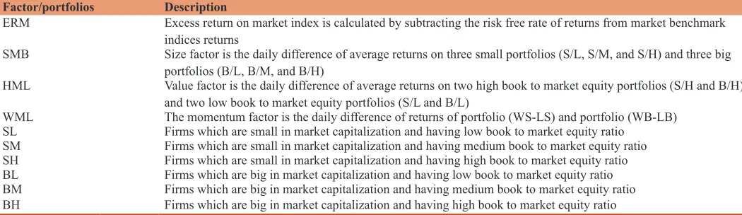
Table 1: Description of pricing factors and test portfolios
Factor/portfolios Description
ERM Excess return on market index is calculated by subtracting the risk free rate of returns from market benchmark indices returns
SMB Size factor is the daily difference of average returns on three small portfolios (S/L, S/M, and S/H) and three big portfolios (B/L, B/M, and B/H)
HML Value factor is the daily difference of average returns on two high book to market equity portfolios (S/H and B/H) and two low book to market equity portfolios (S/L and B/L)
WML The momentum factor is the daily difference of returns of portfolio (WS-LS) and portfolio (WB-LB) SL Firms which are small in market capitalization and having low book to market equity ratio
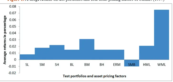
4.1. Descriptive Statistics
The Table 2 presents the descriptive statistics of six test portfolios (SL, SM, SH, BL, BM and BH), and the four asset pricing factors (ERM, SMB, HML and WML). In our sample period, the size
factor has generated negative average daily returns of −0.010 while
the other three factors i.e. ERM, HML and WML have generated
average daily returns of 0.015, 0.021 and 0.075 respectively.
Similarly, the average daily returns given by six test portfolios
i.e., SL, SM, SH, BL, BM, BH are 0.008, 0.018, 0.022, 0.015, 0.031 and 0.015 respectively (Figure 1). All the variables are
normally distributed as the Jarque-Bera test statistics is statistically
significant for all the variables (P<0.05).
4.2. The Correlation Coefficients amongst Pricing
Factors
The Table 3 represents the correlation coefficients amongst the
size, value, momentum and the market factor. The ERM factor is
having very low correlation coefficients value of 0.023, −0.360 and −0.107 with HML, SMB and WML factors respectively. Similarly, the factor HML is also having low correlation coefficient value of 0.155 and −0.075 with SMB and WML factors respectively.
The size factor has documented very low negative correlation of
−0.005 with WML. Thus all the pricing factors are having very low
correlation with each other and provide indication of no problem of multicollinearity problem in the sample.
4.3. Pricing Ability of Carhart (1997) Four Factor Model
The present section provides the results of regression analysis conducted to test the pricing ability of all four factors using OLS and quantile regression. The results for all six test portfolios are as follows.
4.3.1. Test portfolio SL returns
The results of pooled cross-sectional regression analysis conducted to test the pricing ability of Carhart (1997) asset pricing model on test portfolio SL using OLS and quantile regression are presented in Table 4. The panel 1 of the table shows the OLS
results (coefficients followed by standard error) while panels 2-6
display the results of quantile regression at 5th, 25th, 50th, 75th, and 95th percentile levels respectively. From panel 1, the regression
coefficients of all four asset pricing factors ERM, SMB, HML and WML found significant at 1% level of significance with coefficient value of 0.907, 0.543, 0.158 and −0.032 respectively. These four factors explain 90.3% variation in the dependent variable (SL)
thus in this context, it can concluded that the four factor model
holds significant in India.
The significance of these pricing factors in explaining the returns
of test portfolio SL holds robust at all 5 percentile levels except
the ERM factor, which is not best fit beyond 85% percentile and
Table 2: Descriptive statistics of the test portfolios and pricing factors
Statistics SL SM SH BL BM BH ERM SMB HML WML
Mean 0.008 0.018 0.022 0.015 0.031 0.015 0.015 −0.010 0.021 0.075
Median 0.053 0.046 0.030 0.048 0.056 −0.072 0.073 0.026 −0.031 0.127
Maximum 7.316 9.372 14.564 15.816 15.281 24.723 14.922 6.040 9.625 7.774
Minimum −10.262 −10.555 −10.392 −11.537 −14.413 −22.174 −11.478 −9.656 −8.252 −7.832
Standard
deviation 1.363 1.497 1.669 1.517 1.890 2.861 1.503 0.956 1.072 1.148
Skewness −0.485 −0.351 0.082 −0.160 0.034 0.519 −0.234 −0.331 0.577 −0.370
Kurtosis 7.079 7.036 7.088 9.380 8.047 11.125 8.920 7.359 8.663 8.597
Jarque-Bera 3672.047 3504.571 3496.260 8522.688 5319.892 14010.260 7364.391 4058.869 6975.529 6656.067
P 0.000 0.000 0.000 0.000 0.000 0.000 0.000 0.000 0.000 0.000
Sum 38.103 88.349 107.910 77.472 157.819 74.127 76.793 −48.313 105.497 374.894 Sum squared
deviations 9304.335 11227.170 13955.490 11532.990 17905.530 41018.750 11312.660 4575.205 5753.231 6598.734
The sample is from 1st December 1993 to 31st March 2016. The factors SL, SM, SH, BL, BM and BH are the test portfolios are ERM, SMB, HML and WML are pricing factors of
Carhart (1997) four factor model. OLS: Ordinary least square
HML factor is also not good fit in between 75% to 85% percentile
levels (Figure 2).
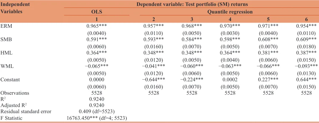
4.3.2. Test portfolio SM returns
In continuation to previous analysis, the Table 5 presents the results of pooled cross-sectional regression analysis conducted to test
the pricing ability of Carhart (1997) asset pricing model on test portfolio SM using OLS and quantile regression. The portfolio SM is average daily reruns on those variables which are having small market capitalization and medium book to market equity
ratio. From panel 1, the regression coefficients of all four asset pricing factors ERM, SMB, HML and WML found significant at 1% level of significance with coefficient value of 0.957, 0.593, 0.348, and −0.041 respectively. The goodness of fit for this model is 0.924 indicating that these four factors explain 92.4% variation
in the dependent variable (SM).
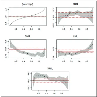
If we Figure 3, the OLS model is not best fit as the SMB factor is
not able to explain the dependent variable beyond 50th percentile
level. Similarly, the HML factor is also not best fit in between
40th and 60th percentiles. The factor WML is also not showing good
Table 3: Correlation coefficient amongst pricing factors
ERM HML SMB WML
ERM 1 0.023762 −0.36035 −0.10709
HML 0.023762 1 0.155357 −0.07542
SMB −0.36035 0.155357 1 −0.00545
WML −0.10709 −0.07542 −0.00545 1
The sample is from 1st December 1993 to 31st March 2016. The factors ERM, SMB,
HML and WML are pricing factors of Carhart (1997) four factor model. OLS: Ordinary least square
Table 4: Regression results four factor model using returns of SL portfolio as dependent variable
Independent
Variables OLS Dependent variable: Test portfolio (SL) returnsQuantile regression
1 2 3 4 5 6
ERM 0.907***
(0.0040) 0.897***(0.0110) 0.900***(0.0050) 0.901***(0.0040) 0.904***(0.0040) 0.926***(0.0130)
SMB 0.543***
(0.0070) 0.556***(0.0160) 0.543***(0.0070) 0.536***(0.0060) 0.533***(0.0080) 0.544***(0.0210)
HML 0.158***
(0.0050) 0.145***(0.0130) 0.159***(0.0060) 0.159***(0.0050) 0.171***(0.0060) 0.154***(0.0180)
WML −0.032***
(0.0050) −0.038***(0.0140) −0.028***(0.0060) −0.023***(0.0050) −0.030***(0.0050) −0.038**(0.0170)
Constant 0.0040
(0.0060) −0.656***(0.0160) −0.235***(0.0060) (0.0060)−0.010 0.226***(0.0070) 0.667***(0.0190)
Observations 5528 5528 5528 5528 5528 5528
R2 0.9030
Adjusted R2 0.9030
Residual standard error 0.418 (df=5523) F Statistic 12859.760*** (df=5523)
**P<0.05; ***P<0.01. The sample is from 1st December 1993 to 31st March 2016. The table represents the results of OLS (in panel 1) and quantile regression
(in panel 2 to 6 for 5th, 25th, 50th, 75th and 95th percentile respectively. The portfolio returns of SL are taken as dependent variable. The coefficients are reported opposite to the
variable (Right side, below the respective panel) followed by standard error. OLS: Ordinary least square
Table 5: Regression results four factor model using returns of SM portfolio as dependent variable
Independent
Variables OLS Dependent variable: Test portfolio (SM) returnsQuantile regression
1 2 3 4 5 6
ERM 0.965***
(0.0040) 0.957***(0.0110) 0.968***(0.0050) 0.970***(0.0030) 0.971***(0.0040) 0.954***(0.0110)
SMB 0.591***
(0.0060) 0.593***(0.0160) 0.584***(0.0070) 0.598***(0.0050) 0.608***(0.0070) 0.609***(0.0180)
HML 0.364***
(0.0050) 0.348***(0.0120) 0.348***(0.0050) 0.364***(0.0040) 0.381***(0.0060) 0.387***(0.0150)
WML −0.065***
(0.0050) −0.041***(0.0120) −0.060***(0.0060) −0.063***(0.0050) −0.066***(0.0060) −0.093***(0.0130)
Constant 0.0000
(0.0060) −0.644***(0.0160) −0.224***(0.0070) (0.0050)0.0002 0.227***(0.0070) 0.644***(0.0150)
Observations 5528 5528 5528 5528 5528 5528
R2 0.9240
Adjusted R2 0.9240
Residual standard error 0.409 (df=5523) F Statistic 16763.450*** (df=4; 5523)
** shows significant at 5% level of significance (p<0.05) while *** indicates significant at 1% level of significance (p<0.01). The sample is from 1st December 1993 to 31st March 2016.
The table represents the results of OLS (in panel 1) and quantile regression (in panel 2 to 6 for 5th, 25th, 50th, 75th and 95th percentile respectively. The portfolio returns of SM are taken as
fit for top percentile SM portfolio returns (beyond 80th percentile)
and bottom percentile SM portfolio returns (below 20th percentile).
4.3.3. Test portfolio SH returns
Further, the similar analysis was conducted after taking SH portfolio returns as dependent variable and the results are reported in Table 6. The results of OLS from panel 1 of Table 6 show the
regression coefficients of all four asset pricing factors ERM, SMB, HML and WML as 1.015, 0.736, 0.668, and 0.0010 respectively. These coefficients are significant at 1% level of significance except the coefficient of WML factor. These four factors explain 96.8%
variation in the dependent variable (SH). In consistent to previous analysis conducted for SL and SM dependent variables, the WML
factor has become insignificant now for dependent variable SH.
The WML factor is significant only at 25th percentile level. If we
see the fitting lines of both OLS and quantile regression (Figure 4),
the SMB factor is not appearing good fit with OLS fitting line as
the straight line is not modeling it completely. Similarly, the factor HML is not able to model the dependent variable (SH) returns for
below 60th percentile and above 80th percentile levels. The WML
is also not best fit below 50th percentile levels.
4.3.4. Test portfolio BL returns
The Table 7 reports the results of the similar analysis conducted after taking the return of BL portfolio returns. The panel 1 of
Table 7 shows the regression coefficients of all four asset pricing factors ERM, SMB, HML and WML as 0.987, −0.048, −0.102 and 0.008 respectively. These coefficients are significant at 1% level of significance except the coefficient of WML factor which
loses the significance beyond 75th percentile level (panel 5 and
6 of table). These four factors explain 98.2% variation in the dependent variable (BL).
Figure 3: The fitting lines of ordinary least square and quantile regression for dependent variable SM and independent factors (ERM, SMB, HML and WML)
From Figure 5, the OLS fitting line is not sufficient enough to
gauge the impact of ERM factor on dependent variable BL below
70th percentile level. It is only fitting well above 70th percentile
level. The SMB factor is also not showing good fit with OLS line
except for 40-75th percentile. The factor HML is also not fitted
well below 20th percentile level.
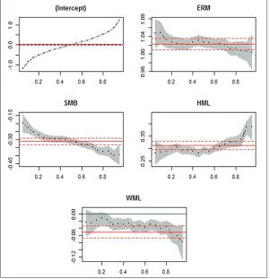
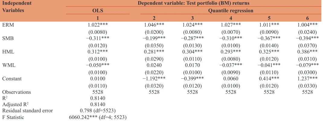
4.3.5. Test portfolio BM returns
In consistent with existing analysis conducted for four variables (SL, SM, SH and BL) the OLS results for BM (Table 8) are also
not best fit across all quantile levels. From Figure 6, it is evident
that SMB factor is not best fit below 25th percentile level and above
60th percentile level. The factor WML is also not best fit for below
20th percentile level and HML for 80th percentile level.
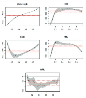
4.3.6. Test portfolio BH return
The OLS results reported in Table 9 are having low R2 value
of 0.259 which indicates that the model is not best fit and only
explains 25.9% variation in the dependent variable (BH portfolio
returns) (Figure 7). The OLS line is also not able to fit SMB and HML across all quantile levels and factor ERM is not fitted for
below 20th percentile level.
5. FINDINGS AND CONCLUSIONS
The results reported in section 4.3 have shown the pricing ability of Carhart (1997) four factor model using six test portfolios as dependent variables. The results have indicated
that the four factor model explain significant variation in the
Table 6: Regression results four factor model using returns of SH portfolio as dependent variable
Independent
Variables OLS Dependent variable: Test portfolio (SH) returnsQuantile regression
1 2 3 4 5 6
ERM 1.015***
(0.0030) 1.007***(0.0070) 1.014***(0.0030) 1.018***(0.0020) 1.016***(0.0030) 1.014***(0.0090)
SMB 0.736***
(0.0050) 0.767***(0.0120) 0.730***(0.0040) 0.713***(0.0040) 0.714***(0.0050) 0.726***(0.0140)
HML 0.668***
(0.0040) 0.659***(0.0100) 0.655***(0.0040) 0.658***(0.0030) 0.669***(0.0040) 0.697***(0.0110)
WML 0.0010
(0.0040) (0.0090)0.0040 0.013***(0.0030) (0.0030)0.0040 (0.0040)0.0050 (0.0120)0.0060
Constant 0.0010
(0.0040) −0.453***(0.0110) −0.158***(0.0040) (0.0040)−0.007 0.153***(0.0050) 0.469***(0.0140)
Observations 5528 5528 5528 5528 5528 5528
R2 0.9680
Adjusted R2 0.9680
Residual standard error 0.295 (df=5523) F Statistic 42178.870*** (df=4; 5523)
** shows significant at 5% level of significance (p<0.05) while *** indicates significant at 1% level of significance (p<0.01). The sample is from 1st December 1993 to 31st March 2016.
The table represents the results of OLS (in panel 1) and quantile regression (in panel 2 to 6 for 5th, 25th, 50th, 75th and 95th percentile respectively. The portfolio returns of SH are taken as
dependent variable. The coefficients are reported opposite to the variable (Right side, below the respective panel) followed by standard error. OLS: Ordinary least square
Table 7: Regression results four factor model using returns of BL portfolio as dependent variable
Independent
Variables OLS Dependent Variable: Test portfolio (BL) returnsQuantile regression
1 2 3 4 5 6
ERM 0.987***
(0.0020) 0.986***(0.0040) 0.993***(0.0020) 0.993***(0.0020) 0.990***(0.0020) 0.990***(0.0060)
SMB −0.048***
(0.0030) −0.039***(0.0090) −0.037***(0.0030) −0.041***(0.0020) −0.050***(0.0030) −0.069***(0.0100)
HML −0.102***
(0.0030) −0.126***(0.0060) −0.103***(0.0020) −0.097***(0.0020) −0.096***(0.0020) −0.097***(0.0080)
WML 0.008***
(0.0020) (0.0070)0.014** 0.006***(0.0020) 0.006***(0.0020) (0.0020)0.0030 (0.0080)0.0090
Constant 0.0020
(0.0030) −0.300***(0.0090) −0.086***(0.0030) (0.0020)0.004 0.094***(0.0030) 0.293***(0.0090)
Observations 5528 5528 5528 5528 5528 5528
R2 0.9820
Adjusted R2 0.9820
Residual standard error 0.202 (df=5523) F Statistic 73370.340*** (df=4; 5523)
** shows significant at 5% level of significance (p<0.05) while *** indicates significant at 1% level of significance (p<0.01). The sample is from 1st December 1993 to 31st March 2016.
The table represents the results of OLS (in panel 1) and quantile regression (in panel 2 to 6 for 5th, 25th, 50th, 75th and 95th percentile respectively. The portfolio returns of BL are taken as
Figure 5: The fitting lines of ordinary least square and quantile regression for dependent variable BL and independent factors (ERM, SMB, HML and WML)
dependent variables. The results of all three factors ERM, SMB and HML are robust for all sample portfolios but same is not the case with WML factor as it loses its pricing ability for dependent variable SH, BL, BM and BH. The study also compares the OLS results with quantile regression to see
whether the OLS fitting line is best for all the explanatory
variables across all the quantiles. The results show that all
four factors are not best fit using OLS as these factors are not fitting well at different percentile/quantile levels. The size factor (SMB) is not fitting well with OLS for test portfolios SH, SM
(beyond 50th percentile), BL, BM (less than 25th percentile
and above 60th percentile) and BH. Similarly, the HML factor
is not good fit for SH and BH test portfolios. The ERM factor is fitting well across all quantiles with OLS except BL test portfolio. The factor WML is also not best fit with OLS for
SM (below 20th percentile and above 80th percentile) and SH
(below 50th percentile) dependent variables.
In light of the results reported above, we can conclude that the pricing ability of four factor model using daily data holds
significant for data of Indian firms. The results of OLS are robust
and falls in line with the results of quantile regression conducted for 5th, 25th, 50th, 75th, and 95th percentile levels. In contrast to this,
the fitting lines of OLS model fail to model the pricing ability
of independent variables for all the quantile levels. Thus we can conclude that the returns are not distributed in perfect linear form and the OLS fails to model those returns series which are having
fat tails. Thus based on the findings of this study, it is suggested to
use quantile regression to model the asset pricing models as it holds it superiority for modeling the data across all quantile period. The
Table 9: Regression results four factor model using returns of BH portfolio as dependent variable
Independent
Variables OLS Dependent variable: Test portfolio (BH) returnsQuantile regression
1 2 3 4 5 6
ERM 254.724***
(11.7470) (12.5560)14.6150 267.300***(23.7080) 296.050***(11.0170) 284.281***(7.3020) 249.323***(14.0210)
SMB −316.823***
(18.4800) (20.5050)23.8050 −468.784***(41.9850) −406.866***(14.0510) −274.188***(10.4460) −110.895***(16.5280)
HML 421.709***
(15.3350) 60.857***(16.4750) 536.521***(34.9690) 488.503***(11.1270) 444.728***(7.9090) 245.623***(13.7880)
WML −65.987***
(14.5230) (15.2240)9.0250 (30.3340)−50.582 −89.911***(14.6310) −58.387***(8.6690) (17.2190)−33.103
Constant 2493.897***
(16.0110) 279.242***(19.7520) 1721.934***(37.9370) 2713.807***(17.7800) 3328.085***(16.5260) 4162.914***(23.0260)
Observations 5528 5528 5528 5528 5528 5528
R2 0.259
Adjusted R2 0.259
Residual standard error 1186.173 (df=5523) F statistic 482.927*** (df=4; 5523)
** shows significant at 5% level of significance (p<0.05) while *** indicates significant at 1% level of significance (p<0.01). The sample is from 1st December 1993 to 31st March 2016.
The table represents the results of OLS (in panel 1) and quantile regression (in panel 2 to 6 for 5th, 25th, 50th, 75th and 95th percentile respectively. The portfolio returns of BH are taken as
dependent variable. The coefficients are reported opposite to the variable (Right side, below the respective panel) followed by standard error. OLS: Ordinary least square Table 8: Regression results four factor model using returns of BM portfolio as dependent variable
Independent
Variables OLS Dependent variable: Test portfolio (BM) returnsQuantile regression
1 2 3 4 5 6
ERM 1.022***
(0.0080) 1.046***(0.0200) 1.024***(0.0080) 1.027***(0.0070) 1.011***(0.0090) 1.004***(0.0240)
SMB −0.311***
(0.0120) −0.199***(0.0350) −0.287***(0.0130) −0.310***(0.0100) −0.367***(0.0140) −0.394***(0.0370)
HML 0.312***
(0.0100) 0.281***(0.0290) 0.304***(0.0110) 0.293***(0.0080) 0.325***(0.0120) 0.386***(0.0310)
WML −0.050***
(0.0100) (0.0220)0.0240 (0.0100)0.0170 −0.037***(0.0090) −0.041***(0.0110) −0.079***(0.0300)
Constant 0.0100
(0.0110) −1.192***(0.0320) −0.399***(0.0120) (0.0100)0.0060 0.414***(0.0120) 1.237***(0.0330)
Observations 5528 5528 5528 5528 5528 5528
R2 0.8140
Adjusted R2 0.8140
Residual standard error 0.798 (df=5523) F Statistic 6060.242*** (df=4; 5523)
** shows significant at 5% level of significance (p<0.05) while *** indicates significant at 1% level of significance (p<0.01). The sample is from 1st December 1993 to 31st March 2016.
The table represents the results of OLS (in panel 1) and quantile regression (in panel 2 to 6 for 5th, 25th, 50th, 75th and 95th percentile respectively. The portfolio returns of BM are taken as
results of the study fall in consistent with the study conducted by
Allen et al. (2011) which documented the superiority of quantile
regression over OLS while testing Fama and French (1993) three factor asset pricing model.
REFERENCES
Agarwalla, S.K., Jacob, J., Varma, J.R. (2013), Four Factor Model in Indian Equities Market. W.P. No. 2013-09-05. Ahmedabad: Indian Institute of Management.
Allen, D.E., Singh, A.K., Powell, R. (2011), Asset pricing, the Fama-French factor model and the implications of quantile regression analysis. In: Gregoriou, G.N., Pascalau, R., editors. Financial Econometrics Modeling: Market Microstructure, Factor Models and Financial Risk Measures. UK: Palgrave Macmillan. p176-193. Ansari, V.A. (2000), Capital asset pricing model: Should we stop using
it. Vikalpa, 251, 55-64.
Bahl, B. (2006), Testing the Fama and French Three-Factor Model and Its Variants for the Indian Stock Returns. Available from: http://www. ssrn.com/abstract=950899.
Barnes, M., Hughes, W.A. (2002), Quantile Regression Analysis of the
Cross Section of Stock Market Returns, Working Paper. Boston: Federal Reserve Bank. Available from: http://www.ssrn.com/ abstract=458522.
Bassett, G., Chen, H. (2001), Quantile style: Return-based attribution using regression quantiles. Empirical Economics, 26, 293-305. Basu, D., Chawla, D. (2010), An empirical test of CAPM-the case of
Indian stock market. Global Business Review, 11, 209-220. Black, F. (1993), Beta and return. Journal of Portfolio Management,
20, 8-18.
Buchinsky, M., Phillip, L. (1997), Educational Attainment and the Changing US Wage Structure: Some Dynamic Implications, Brown University, Department of Economics Working Paper.
Carhart, M.M. (1997), On persistence in mutual fund performance. Journal of Finance, 52, 57-82.
Chan, L.K.C., Lakonishok, J. (1992), Robust measurement of beta risk. The Journal of Financial and Quantitative Analysis, 27(2), 265-282. Choudhary, K., Choudhary, S. (2010), Testing capital asset pricing model:
Empirical evidences from Indian equity market Eurasian. Journal of Business and Economics, 36, 127-138.
Chui, A., Titman, S., Wei, K.C.J. (2000), Momentum, ownership structure, and financial crises: An analysis of Asian stock markets. Working Paper: University of Texas at Austin.
Conner, G., Sehgal, S. (2001), Tests of the Fama-French Model in India, Working Paper Series.
Connor, G., Sehgal, S. (2003), Tests of the Fama and French model in India. Decision, 302, 1-20.
Engle, R. F., Manganelli, S. (1999), CAViaR: Conditional value at risk by quantile regression, National Bureau of Economic Research Working Paper No. 7341.
Fama, E.F., French, K.R. (1992), The cross-section of expected stock returns. Journal of Finance, 47, 129-176.
Fama, E.F., French, K.R. (1993), Common risk factors in the returns on stocks and bonds. Journal of Financial Economics, 33, 3-56. Fama, E.F., French, K.R. (1996), Multifactor explanations of asset pricing
anomalies. Journal of Finance, 51, 55-84.
Grundy, B.D., Martin, J.S. (2001), Understanding the nature of the risks and the source of the rewards to momentum investing. Review of Financial Studies, 14(1), 29-78.
Gupta, O.P., Sehgal, S. (1993), An empirical testing of capital asset pricing model in India. Finance India, 74, 863-874.
Horowitz, J.L., Loughran, T., Savin, N.E. (2000), Three analyses of the firm size premium. Journal of Empirical Finance, 7, 143-153. Officer, R. R. (1972), The Distribution of Stock Returns, Journal of the
American Statistical Association, 67, 340.
Jegadeesh, N., Titman, S. (1993), Returns to buying winners and selling losers: Implications for stock market efficiency. Journal of Finance, 48, 65-91.
Jegadeesh, N., Titman, S. (2001), Profitability of momentum strategies: An evaluation of alternative explanations. The Journal of Finance, 56(2), 699-720.
Knez, P.J., Ready, M.J. (1997), On the robustness of size and book-to-market in cross-sectional regressions. The Journal of Finance, 52, 1355-1382.
Koenker, R.W., Bassett, G. (1978), Regression quantiles. Econometrica, Econometric Society, 46(1), 33-50.
Kothari, S., Shanken, J. (1995), In defense of beta. Journal of Applied Corporate Finance, 8, 53-58.
Levhari, D., Levy, H. (1977), The capital asset pricing model and the investment horizon. Review of Economics and Statistics, 59, 92-104. Lintner, J. (1965), The valuation of risk assets and the selection of risky
investments in stock portfolios and capital budgets. Review of Economics and Statistics, 47, 13-37.
Ma, L., Pohlman, L. (2008), Return forecasts and optimal portfolio construction: A quantile regression approach. The European Journal of Finance, 14(5), 409-425.
Madhusoodanan, T.P. (1997), Risk and return: A new look at the Indian stock market. Finance India, 112, 285-304.
Manjunatha, T., Mallikarjunappa, T. (2009), Bivariate analysis of capital
asset pricing model in Indian capital market. Vikalpa, 34, 47-59. Manjunatha, T., Mallikarjunappa, T. (2011), Does three factor model
explain asset pricing in Indian capital market? Decision, 38, 119-140. Manjunatha, T., Mallikarjunappa, T., Begum, M. (2006), Does Capital
Asset Pricing Model Hold in the Indian Market? Indian Journal of Commerce, 59(2), 73-83.
Morillo, D.S. (2000), Monte Carlo American Option Pricing with Nonparametric Regression, in: Essays in Nonparametric Econometrics, Dissertation, University of Illinois.
Nair, A.S., Sarkar, A., Ramanathan, A., Subramanyam, A. (2009), Anomalies in CAPM: A panel data analysis under Indian conditions. International Research Journal of Finance and Economics, 33, 192-206.
Nartea, G.V., Ward, B.D., Djajadikerta, H.G. (2009), Size, BM, and momentum effects and the robustness of the Fama-French three-factor model: Evidence from New Zealand. International Journal of Managerial Finance, 5(2), 179-200.
Rao, S.N. (2004), Risk factors in the Indian capital markets. The ICFAI Journal of Applied Finance, 10(11), 5-15.
Rouwenhorst, K.G. (1998), International momentum strategies. Journal of Finance, American Finance Association, 53(1), 267-284, 02. Rouwenhorst, K.G. (1999), Local return factors and turnover in emerging
stock markets. Journal of Finance, American Finance Association, 544, 1439-1464, 08.
Sehgal, S. (2003), Common factors in stock returns: The Indian evidence. The ICFAI Journal of Applied Finance, 91, 5-16.
Sharma, P., Kumar, B. (2016), Idiosyncratic volatility and cross-section of stock returns: Evidences from India. Asian Journal of Finance and Accounting, 8(1), 1-12.
Sharpe, W.F. (1964), Capital asset prices: A theory of market equilibrium under conditions of risk. Journal of Finance, 19, 424-444.
Srinivasan, S. (1988), Testing of capital asset pricing model in Indian environment. Decision, 151, 51-59.
Taneja, Y.P. (2010), Revisiting Fama French three factor model in Indian stock market. Vision: The Journal of Business Prespective, 14(4), 267-274. Taylor, J.B. (2000), Low inflation, pass-through, and the pricing power
of firms. European Economic Review, 44(7), 1389-1408.
Treynor, J.L. (1961), Toward a theory of market value of risky assets. In: Korajczyk, R.A., editor. Asset Pricing and Portfolios Performance: Models, Strategy and Performance Metrics. London: Risk Books. Vaidyanathan, R. (1995), Capital asset pricing model: The Indian context.
The ICFAI Journal of Applied Finance, 12, 221-224.
Varma, J.R. (1988), Asset Pricing Model Under Parameter Non-Stationarity, Doctoral Dissertation. Ahmedabad: Indian Institute of Management. Yalwar, Y.B. (1988), Bombay stock exchange: Rates of return and