JIEM, 2019 – 12(2): 340-355 – Online ISSN: 2013-0953 – Print ISSN: 2013-8423 https://doi.org/10.3926/jiem.2742
An Integrated Model for Adjustment of Process Parameters to Recover
Throughput Shortage in Semiconductor Assembly: A Case Study
Ho Kok Hoe1 , Joshua Prakash1 , Shahrul Kamaruddin2 , Ong Kok Seng1 1Universiti Tunku Abdul Rahman (Malaysia)
2Universiti Teknologi Petronas (Malaysia)
[email protected], [email protected], [email protected], [email protected]
Received: September 2018
Accepted: May 2019
Abstract:
Purpose: Existing productivity improvements activities such as inventory buffer, overall equipment effectiveness (OEE) and total productive maintenance (TPM) do not associate the throughput shortage with the process parameters. The paper aims to develop and validate an integrated model to recover the throughput shortage through adjustment of process parameters in a semiconductor assembly setting.
Design/methodology/approach: The mathematical model of planned throughput as a function of process parameters in an integrated multiple-process line is developed. When the actual throughput does not meet the planned throughput, throughput shortage occurs. The planned throughput for the next day is summed with the throughput shortage from the previous day, and mathematical programming is used to search the adjusted values of the process parameters.
Findings: The throughput shortage can be restored at the following day with the reconfigured process parameters. If throughput shortage still exists, the additional throughput shortage will be carried forward to the subsequent day of planning where mathematical programming is repeated to search the adjusted values of the process parameters. The proposed optimisation model is essentially a parametric model, where actual data of process parameters are fitted into distribution and is translated into a range of allowable values within the 95% confidence interval.
Research limitations/implications: The process parameters subject to adjustment in this model are the cycle time of Die Attach, Wire Bond and Pre-Cap Inspection. Downtime and setup time are not subjected to adjustments because these parameters require more extensive efforts to be changed.
Practical implications:The mathematical programming computes adjusted values of process parameters to restore the throughput shortage, where it quantitatively correlates the process parameters and throughput shortage, rather than the conventional method of production improvement activities that do not quantitatively correlate with the throughput shortage.
Originality/value: The research addresses the adjustment of process parameters to recover the throughput shortage in integrated multiple-process line.
To cite this article:
Hoe, H.K., Prakash, J., Kamaruddin, S., & Seng, O.K. (2019). An integrated model for adjustment of process parameters to recover throughput shortage in semiconductor assembly: A case study. Journal of Industrial Engineering and Management, 12(2), 340-355. https://doi.org/10.3926/jiem.2742
1. Introduction
Nowadays, manufacturing industries are facing rising production cost, which creates an urgent need to manage throughput shortage in manufacturing systems. The effectiveness in managing throughput shortage is essential in reducing manufacturing cost (Tekin & Sıtkı, 2012). Throughput shortage manifests itself as the actual throughput is lower than the planned throughput (Gram, 2013). The potential causes of throughput shortage are unplanned machine breakdown, long setup, low production speed, high rework, and long start-up delay. Production control will always attempt to salvage the throughput shortage with the available resources.
There are various ways to recover throughput shortage. The first method is to create an inventory buffer. If the inventory buffer is not available to compensate for throughput deficiencies, the demand is lost or backordered at a relevant cost (Sana, 2012). The allocation of inventory buffer is needed to decouple processes with different production rates, caused by varying cycle times, machine breakdown, short stoppages and material shortage (Sana, 2012). This allocation is vital to sustain the operations of a manufacturing system. There are extensive studies related to the allocation of inventory buffer in production lines, such as by Enginarlar, Jingshan-Li and Zhang (2002), Miltenburg (2000) and Salameh and Ghattas (2001). In addition, Zequeira, Prida and Valdes (2004) developed a production-inventory model to search for optimal production periods between maintenance activities and the corresponding inventory buffer size to meet demand. Sana and Chaudhuri (2010) built a model for the production policy (resumption and non-resumption) to meet optimal safety stock, production rate and production lot size. Although the method ensures the production line continues running smoothly by maintaining sufficient work-in-process (WIP), there is the risk in inducing high holding cost and excessive WIP built-up due to excess buffer (Chan, Tasmin, Aziati, Rasi, Ismail & Yaw, 2017; Nemtajela & Mbohwa, 2017). If the buffer size is low, it may cause machine idling and underutilization which will delay processing, and unable to meet the due date. If the buffer size is sufficient, the machine is well decoupled, and the productivity is maximised.
Another method to recover throughput shortage is through improvement activities such as Overall Equipment Effectiveness (OEE), Total Productive Maintenance (TPM) and lean methodology. OEE and TPM are closely related to the gap between the actual and ideal performance of a manufacturing system. It focuses on three components which are availability, productivity, and quality. Most researches address the reduction of throughput shortage by improving efficiency in a manufacturing system. Tekin and Sıtkı (2012), Gram (2013) and Hassani and Hashemzadeh (2015) find and minimise the throughput shortage by adopting Overall Equipment Effectiveness (OEE) and Balance Score Card approach. The reduction of throughput shortage is examined through the identification of the root causes and specific measures to reduce the throughput shortage. Another method is the reduction of manufacturing wastes by adopting lean tools (Prajapati & Deshpande, 2015; Siva, Patan, Kumar, Purusothaman, Pitchai & Jegathish, 2017). Although the ideal cycle time represents the maximum theoretical speed of the equipment, the equipment may slow down and affect productivity despite high OEE (Anantharaman & Nachiappan, 2006). The cycle time inefficiencies can be reduced through 5S, Jidoka, Muda, visual management and poka-yoke. Prajapati and Deshpande (2015) reviewed cycle time reduction using lean tools such as Kaizen and ‘Takt’ time analysis. Siva et al. (2017) utilised process improvement by cycle time reduction using lean tools such as visual management tool, poka-yoke, Kaizen and Jidoka.
balanced with the product quality, as higher speed may cause more defects and affect the yield. It will also impact the equipment wear and tear, which will result in higher maintenance cost. Experience in inventory buffer management is particularly influenced by subjective judgement, as it is complex to establish a balanced buffer size between successive processes. In contrast, adjustment of process parameters is more objective and has a direct influence on the throughput.
In this paper, a model to recover the throughput shortage in a two-stage production planning system is proposed. The model links the throughput shortage with process parameters where these parameters can be adjusted within the feasible range. The rationale behind the adjustment of process parameters is to provide satisfactory throughput gain (Wuest, Weimer, Irgens & Thoben, 2016). The cycle time of each process is adjusted to meet the planned throughput, which includes the throughput shortage. This is because the cycle time can be controlled while other process parameters such as downtime and setup time are stochastic, hence impractical to be adjusted (Sharma & Jain, 2015; Xu, Zhao, Wu, Zhou, Ma & Liu, 2016). Setup time on a machine is stochastic when there is variability in the length of setup time due to inconsistency in adjacent product types (Xu et al., 2016). In practice, the machine cycle time can be adjusted within an allowable range by adjusting the machine setting such as indexing time, delay in pick-up, delay in bonding, and bond time. The proposed model can create a relationship between throughput shortage and process parameters where these parameters are subject to changes in the manufacturing system. The parametric model uses input data of process parameters based on distributions that are translated into a range of allowable values within the 95% confidence interval. The extension of this benefit leads to effective production planning to recover the throughput shortage through better computation between improvement activities and manufacturing parameters. The proposed model is established to accommodate existing practise in production planning, throughput shortage recovery, and productivity improvement.
Section 1 reviews existing methods to recover the throughput shortage and their limitations. Section 2 presents the outline of the model used in this study. Section 3 describes the development of the proposed model. Section 4 validates the proposed model. Section 5 discusses the impact of the throughput shortage recovery using the proposed model. The conclusion drawn from the result is presented in Section 6.
2. The Two-Stage Integrated Production Planning Model
The proposed production planning model is used to plan daily throughput and recover throughput shortage concurrently in a real-time manufacturing scenario. The model is divided into two stages: daily throughput planning in the 1st stage and throughput shortage recovery in the 2nd stage. The 1st stage estimates throughput using the mathematical model of planned throughput and is compared with the corresponding actual throughput. When there is throughput shortage (actual throughput less than planned throughput), the throughput shortage (difference in actual and planned throughput) is included in the subsequent day planning at the 2nd stage. In the 2nd stage, mathematical programming searches the optimum values of process parameters to meet the new projected throughput. However, if there is throughput shortage even after adjustment of process parameters, the throughput shortage will be included in subsequent day planning at the 2nd stage for mathematical programming analysis until no further throughput shortage is encountered.
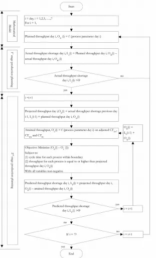
Figure 1 shows the flowchart of the approach adopted in the two-stage production planning model, expressed for a single period of seven days. The planned throughput is a function of process parameters and is based on data mining of the simulated data. The range of values of the process parameters is based on real-time data, fitted into distributions and translated into a range of allowable values within a 95% confidence interval. The data collection of relevant performance measures is based on full factorial runs of a simulation model, and the mathematical model of throughput as a function of process parameters is formulated using regression.
For day i (i = 1,2,…..,7), the planned throughput, OM(i) is compared with actual throughput, ORT(i). If ORT(i) is less than OM(i), the next step is to proceed to the 2nd stage since there is throughput shortage, La(i).
still throughput shortage, Lp(i+1). Thus, the next step is to repeat the mathematical programming procedure for next day (i+2). The predicted throughput shortage, Lp(i+1) is carried forward for the subsequent day (i+2) for the mathematical programming to estimate OC(i+2) that can meet OB(i+2) + Lp(i+1) within the range of values of process parameters. This step is repeated as long as the predicted throughput shortage occurs. If there is no predicted throughput shortage, the 2nd stage production planning is terminated, and the 1st stage production planning is repeated for the subsequent day. The rationale of the methodology is to adjust values of process parameters only when there is throughput shortage or predicted throughput shortage.
The proposed production planning model is made up of the mathematical model of makespan, TB(i), the formulation of a mathematical model of planned throughput, OM (i), and mathematical programming of attained throughput, OC(i).
3. Model Development through a Case Study
The case study was carried out in a semiconductor assembly line which consisted of three die attach machines, four oven cure machines, nine wire bond machines, and three pre-cap inspection machines. Figure 2 shows the process flow and the corresponding parameters in each process.
Die Attach Oven Cure Wire Bond Pre-Cap
Inspection
Cycle Time (CTOC) Cycle Time (CTPC)
Cycle Time (CTDA) Downtime Duration (DDDA) Downtime Frequency (DFDA) Setup Time (STDA)
Cycle Time (CTWB) Downtime Duration (DDWB) Downtime Frequency (DFWB) Setup Time (STWB)
Figure 2. The process parameters for a semiconductor assembly line
Referring to Figure 2, the first process is Die Attach, where the machine processes the wafer into unit form. Each Die Attach machine processes one wafer at a time. The completed units are accumulated in batches before transferred to the next process, Oven Cure, where batches are placed in an oven for curing. Then, the batches are transferred to the next process, Wire Bond, where a wire was placed starting from the die to the lead frame of each unit. The Wire Bond machine processes one unit at one time. The completed units are accumulated in batches before it is sent to the next process, Pre-Cap Inspection, where the quality of each physical unit is inspected. The Pre-Cap Inspection machine inspects one unit at a time, and completed units are accumulated in batches before sent to the next process. In this study, the system ends when the batch completes the Pre-Cap Inspection. Setup is performed once during Die Attach and Wire Bond at the start of each day. An Oven Cure machine can accommodate up to eight batches at a time. No set up is required in Oven Cure and Pre-Cap Inspection.
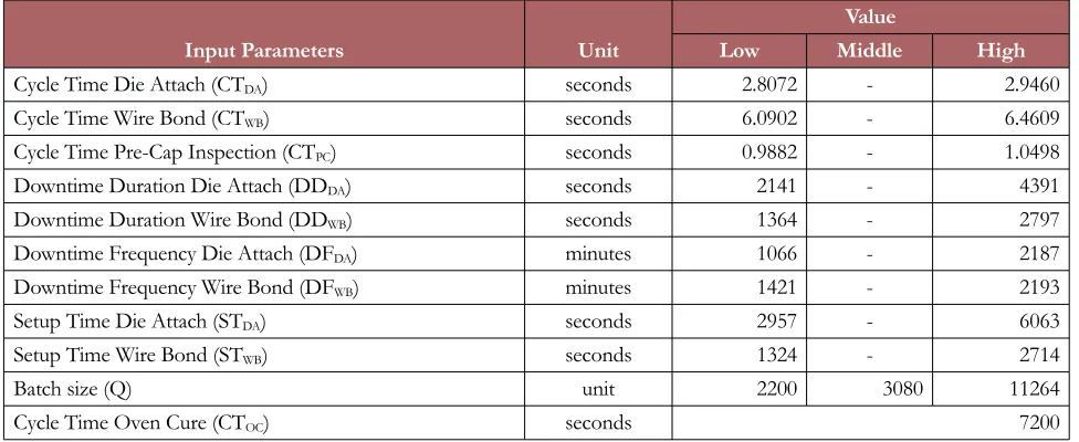
The following stage is to identify the range of values of the process parameters. Table 1 shows the classification of process parameters and their values. The raw data is collected from the manufacturing system database throughout 30 days. The raw data are fitted into normal distribution (for cycle time) and exponential distribution (for downtime duration, downtime frequency and setup time) (Gandhi & Harchol-Balter, 2009). 95% confidence interval of the distribution determines the two levels of the process parameters which are the minimum and maximum. The two levels are further used in setting the range of allowable values during mathematical programming at the 2nd stage.
Input Parameters Unit
Value
Low Middle High
Cycle Time Die Attach (CTDA) seconds 2.8072 - 2.9460
Cycle Time Wire Bond (CTWB) seconds 6.0902 - 6.4609
Cycle Time Pre-Cap Inspection (CTPC) seconds 0.9882 - 1.0498
Downtime Duration Die Attach (DDDA) seconds 2141 - 4391
Downtime Duration Wire Bond (DDWB) seconds 1364 - 2797
Downtime Frequency Die Attach (DFDA) minutes 1066 - 2187
Downtime Frequency Wire Bond (DFWB) minutes 1421 - 2193
Setup Time Die Attach (STDA) seconds 2957 - 6063
Setup Time Wire Bond (STWB) seconds 1324 - 2714
Batch size (Q) unit 2200 3080 11264
Cycle Time Oven Cure (CTOC) seconds 7200
The next step is to develop a mathematical model of makespan, TB and planned throughput, OM using regression. The planned throughput, OM is defined as the total time available in the system divided by the processing time of a unit in the system (Salvendry, 2007; Khan, 2007; Telsang, 2010). The planned throughput, OM can be written as shown in Equation (1).
OM= TTOTAL
TUNIT
(1)
Where:
OM = planned throughput per day TTOTAL = total time available per day TUNIT = processing time per unit
The processing time per unit is the makespan, TB divided by the batch size Q. The makespan, TB is the total length of processing time when all jobs of batch size Q have finished processing. TB is obtained through data collection of 1536 experiment runs (29 × 31 × 11 = 1536) collected from Pro-Model simulation model. The simulation model is built to represent the integrated processes of the semiconductor assembly line, and the process parameters from Table 1 are inserted into the model to obtain Tb for each run. OM can now be calculated using Equation (2).
OM=
TTOTALx Q TR
(2)
Where:
OM = planned throughput per day TTOTAL = total time available per day Q = batch size
TB = makespan
The full factorial runs of TB is inserted into statistical JMP software to formulate a regression model. TB as a function of process parameters is shown in Equation (3).
TB = 7187.5725 + 387.1239 [CTDA0.0694−2.8766]+ 1008.0011 [CTWB0.1854−6.2756]+ 157.9690[CT0.0308PC−1.019]+
9.5167 [DDDA−3266]
1125 + 3.9325
[DDWB−2080.5]
716.5 + 2.4477
[DFDA−1626.5]
560.5 - 0.1807
[DFWB−1807]
386
-2.6148 [STDA−4510]
1553 + 24.3713
[STWB−2019]
695 + 10.1729Q
(3)
Where:
TB = makespan
STDA = setup time Die Attach STWB = setup time Wire Bond Q = batch size
TTOTAL is defined as the total time available per day in the system (Salvendry, 2007; Khan, 2007; Telsang, 2010). TTOTAL is the summation of the individual process time available minus the setup time for each day. M is defined as the number of machines available at each process based on the process with the least capacity in the system. TD is defined as the maximum time per day. ADA is defined as machine availability for Die Attach, and AWB is defined as machine availability for a Wire Bond.
The total time available per day in the system, TTOTAL is written as shown in Equation (4):
TTOTAL = ((TD – STDA)(ADA) + (TD)(1) + (TD – STWB)(AWB)) + (TD)(1)) x (M) (4)
Where:
TD = maximum time per day STDA = setup time Die Attach STWB = setup time Wire Bond ADA = Die Attach availability AWB = Wire Bond availability
M = number of machine available based on the process with least capacity in the system
The availability at Oven Cure and Pre-Cap Inspection is one because there is no downtime defined for these two processes. Besides, no setup is required during Oven Cure and Pre-Cap Inspection. Machine availability, A is defined in Equation (5) (Salvendry, 2007; Khan, 2007; Telsang, 2010).
A= MTBF
MTBF+MTTR (5)
MTTR is defined in Equation (6):
MTTR= Machine Downtime Duration
Machine Downtime Frequency= DDP
(DFP
1440)
(6)
1440 minutes = 24 hours × 60 minutes; p = WB (Wire Bond) or DA (Die Attach); MTBF is defined in Equation (7):
MTBF=86400−Machine Downtime Duration
Machine Downtime Frequency =
86400−DDP
(DFP
1440)
(7)
86400 seconds = 24 hours × 60 minutes × 60 seconds; p = WB (Wire Bond) or DA (Die Attach); Equation (6) and Equation (7) are substituted in Equation (5) and is written as shown in Equation (8).
A=86400−DDP
86400 (8)
OM=
((TD−STDA)(
86400−DDDA
86400 )+(TD)(1)+(TD−STWB)(
86400−DDWB
86400 )+(TD)(1)) x(M)x Q
7187.5725+3871239[CTDA−2.8766]
0.0694 +10+080011
[CTWB−6.2756]
0.1854 +157.9690
[CTPC−1.019] 0.0308
+9.5167[DDDA1125−3266]+3.9325[DDWB716.5−2080.5]+2.4477[DFDA560.5−31626.5]−0.1807[DFWB386−1807]
2.6148[STDA−4510]
1553 +24.3713
[STWB−2019]
695 +10.1729Q
(9)
Step 1: 1st Stage of Production Planning
The validity of the model is tested in three different periods. A single period of the model is defined as seven days (n = 7) where day i (i = 1,2,3,…..,7). For day 1 (i=1), OM(1) is estimated based on Equation (9) as a function of process parameters of day 1. The planned throughput, OM(1) is compared with actual throughput, ORT(1), to assess if there is actual throughput shortage, La(1). If ORT(1) > OM(1), there is no actual throughput shortage and the planned throughput, for day 2, OM(2) is estimated using Equation (9). If there is actual throughput shortage in day 1, where ORT(1) < OM(1), La(1) will be carried forward to the 2nd stage of production planning for day 2. Generally, if the actual throughput shortage for day i, La(i) is zero or negative, the planned throughput for day (i+1), OM(i+1) is estimated using Equation (9). On the other hand, if the actual throughput shortage of day i, La(i) is positive, the throughput shortage will be carried forward to the 2nd stage of production planning for day i+1.
Step 2: 2nd Stage of Production Planning
2nd stage of production planning is involved when there is throughput shortage incurred at the 1st stage of production planning. In the 2nd stage of production planning, the projected throughput of the day i+1, O
B(i+1) is the sum of actual throughput shortage from previous day i, La(i) and planned throughput of the day i+1, OM(i+1). The cycle time of the processes (CTDA, CTWB and CTPC) need to be adjusted to ensure OB(i) is met. The attained throughput for day i+1, OC(i+1) is a function of the adjusted cycle time values (CTDA, CTWB and CTPC) obtained by mathematical programming. This is because the cycle time can be controlled while the downtime and setup time are stochastic, hence impractical to be manipulated. The cycle time can be controlled by the machine settings, such as by changing the delay time or by adjusting the movement mechanism of the machine parts. OB(i+1) is obtained using Equation (10).
If OM(i) - ORT (i) > 0, then OB(i+1) = OM(i+1) + OM(i) - ORT(i) (10)
In the mathematical programming development, the objective function is to minimize the difference between attained throughput of day i+1, OC(i+1) and projected throughput of day i+1, OB(i+1).
The mathematical programming model in the 2nd stage of the model is formulated as follows in Equation (11) to Equation (20):
Objective function:
Minimize OM(i+1) + (OM(i) – ORT(i)) - TTOTALT x Q B
(11)
Constraints:
CTDA(i+1) ≥ 2.8072 (12)
CTDA(i+1) ≤ 2.9460 (13)
CTWB(i+1) ≤ 6.4609 (15)
CTPC(i+1) ≥ 0.9882 (16)
CTPC(i+1) ≤ 1.0498 (17)
[[(86400−STDA(i+1))x(86400 x(86400−DDDA(i+1)))]
CTDA(i+1)
]x 3≥OB(i+1) (18)
[[(86400−STWB(i+1))x(86400 x(86400−DDWB(i+1)))]
CTWB(i+1)
]x9≥OB(i+1) (19)
[(86400 x1)
CTPC(i+1)
]x 3≥OB(i+1) (20)
Equation (11) states that the objective function is to minimise the difference between the attained throughput of day i+1, OC(i+1) and the projected throughput of day i+1, OB(i+1). Equation (12) to Equation (17) ensures that the cycle times fall within the boundary of the allowable values defined in Table 1. Equation (18) to Equation (20) ensures that the throughput for each process is at least equal or higher than OB(i+1). Equation (18) to Equation (20) is important to validate whether OC(i+1) can meet OB(i+1).
If there is no additional predicted throughput shortage, the planned throughput for subsequent day i+2, OM(i+2) is estimated using 1st stage of production planning. If (O
B(i+1) – OC(i+1)) for day i+1 is positive, there is additional predicted throughput shortage at the 2nd stage of production planning. The predicted throughput shortage is carried forward to the subsequent day, and the 2nd stage of production planning is repeated for day i+2 where OC(i+2) is estimated to meet OB(i+2) using mathematical programming. The model is valid for multiple-period as long as the process parameters in each period fall within the range of values shown in Table 1. Three different periods of real-time data are collected to validate the model in a real-time scenario. Each period consists of seven days.
4. Validation of the Proposed Production Planning Model
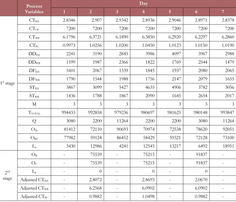
Case Study 1: Period 1Table 2 shows the production planning data obtained for the 1st period of 7 days. For day 1 in the 1st stage of production planning, OM(1) is estimated at 81412 units. ORT(1) is 77982 units. Since OM(1) is higher than ORT(1), there is throughput shortage; thus the throughput shortage of day 1, (La(1)=3430 units) is carried forward to the 2nd stage of production planning. For day 2, OM(2) is estimated at 72110 units. The throughput shortage from day 1, La(1) is added to the planned throughput of day 2, OM(2). OB(2) is calculated as OM(2) + La(1) where it is equal to 75539 units. In the 2nd stage, the mathematical programming assessed the adjusted cycle time within the boundary shown in Table 1 and estimated OC(2) as 75539 units. Since OC(2) is equal to OB(2), there is no predicted throughput shortage that is required to be carried forward to the next day (i=3).
For day 3 in the 1st stage of production planning, O
M(3) is estimated at 90693 units. ORT(1) is 86452 units. Since OM(3) is higher than ORT(3), there is throughput shortage; thus the throughput shortage of day 3, (La(3)=4241 units) is carried forward to the 2nd stage of production planning. For day 4, O
in Table 1 and estimated OC(6) as 91837 units. Since OC(6) is equal to OB(6), there is no predicted throughput shortage that is required to be carried forward to the next day (i=7).
For day 7, OM(7) is estimated at 92051 units, and ORT(7) is 73100. Since OM(7) is higher than ORT(7), there is throughput shortage; thus the throughput shortage of day 7, (La(7)=18951 units) is carried forward to the 2nd stage of production planning for day 8. Since the case study is limited to seven days period, the analysis stops at this point.
Process Variables
Day
1 2 3 4 5 6 7
1st stage
CTDA 2.8346 2.907 2.9342 2.8936 2.9046 2.8971 2.8378
CTOC 7200 7200 7200 7200 7200 7200 7200
CTWB 6.1796 6.3721 6.1890 6.3850 6.2920 6.2297 6.2860
CTPC 0.9973 1.0256 1.0200 1.0450 1.0123 1.0150 1.0190
DDDA 2241 3190 2845 3986 4097 3967 2988
DDWB 1599 1987 2366 1822 1769 2544 1479
DFDA 1601 2067 1339 1845 1937 2080 2065
DFWB 1790 1544 1988 1756 2147 2079 1655
STDA 3867 3099 5427 4635 4906 3782 3056
STWB 1436 1788 1867 2090 1645 2654 2017
M 3 3 3 3 3 3 3
TTOTAL 994433 992858 979236 980697 981625 980148 993847
Q 3080 2200 11264 2200 2200 3080 11264
OM 81412 72110 90693 70974 72538 78620 92051
ORT 77982 59124 86452 58429 59321 72128 73100
La 3430 12986 4241 12545 13217 6492 18951
2nd
stage
OB - 75539 - 75215 - 91837
-OC - 75539 - 75215 - 91837
-Lp - 0 - 0 - 0
-Adjusted CTDA - 2.8072 - 2.8693 - 2.0670
-Adjusted CTWB - 6.2568 - 6.0902 - 6.0902
-Adjusted CTPC - 0.9882 - 1.0498 - 0.9882
-Table 2. 1st Stage and 2nd Stage of Production Planning for 1st Period
Case Study 2: Period 2
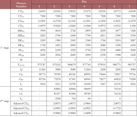
Table 3 shows the production planning data obtained for the 2nd period for 7 days. For day 1 in the 1st stage of production planning, OM(1) is estimated at 90772 units. ORT(1) is 85756 units. Since OM(1) is higher than ORT(1), there is throughput shortage; thus the throughput shortage of day 1, (La(1)=5016 units) is carried forward to the 2nd stage of production planning. For day 2, O
OM(3) is estimated at 80136 units. The predicted throughput shortage from day 2, Lp(2) is added to the planned throughput of day 3, OM(3). OB(3) is calculated as OM(4) + Lp(3) where it is equal to 82684 units. In the 2nd stage, the mathematical programming assessed the adjusted cycle time within the boundary shown in Table 1 and estimated OC(3) as 81980 units. Since OC(3) is lower than OB(3), there is a predicted throughput shortage that is required to be carried forward to the next day (i=4). Lp(3) is 704 units.
Process Variables
Day
1 2 3 4 5 6 7
1st stage
CTDA 2.8432 2.8342 2.9032 2.9178 2.8190 2.8772 2.8100
CTOC 7200 7200 7200 7200 7200 7200 7200
CTWB 6.1901 6.2720 6.1126 6.3301 6.1450 6.3021 6.2378
CTPC 1.0079 0.9220 1.0260 1.0348 0.9972 1.0152 1.020
DDDA 3990 4010 3720 2899 2690 2477 3320
DDWB 2265 2740 1608 1790 2011 2390 2700
DFDA 1205 1580 1945 1540 1766 2010 2087
DFWB 1742 1823 2009 1990 2080 1590 1630
STDA 4932 5109 3550 5742 5230 4480 5020
STWB 2430 2054 2689 2090 2190 1988 1420
M 3 3 3 3 3 3 3
TTOTAL 975787 975532 984679 977745 979935 984775 981757
Q 11264 3080 3080 11264 2200 2200 3080
OM 90772 78789 80136 89995 75844 72967 79716
ORT 85756 73278 67341 68945 72677 60832 75200
La 5016 5511 12795 21050 3167 12135 4516
2nd stage
OB - 83805 82684 90699 - 76134
-OC - 81257 81980 90789 - 76134
-Lp - 2548 704 -90 - 0
-Adjusted CTDA - 2.8072 2.8072 2.9460 - 2.8072
-Adjusted CTWB - 6.0902 6.0902 6.0902 - 6.1722
-Adjusted CTPC - 0.9882 0.9882 1.0498 - 0.9882
-Table 3. 1st Stage and 2nd Stage of Production Planning for 2nd Period
OM(4) is estimated at 89995 units. The predicted throughput shortage from day 3, Lp(3) are added to the planned throughput of day 4, OM(4). OB(4) is calculated as OM(4)+Lp(3) where it is equal to 90699 units. In the 2nd stage, the mathematical programming assessed the adjusted cycle time within the boundary shown in Table 1 and estimated OC(4) as 90789 units. Since OC(4) is higher than OB(4), there is no predicted throughput shortage that is required to be carried forward to the next day (i=5).
in Table 1 and estimated OC(6) as 76134 units. Since OC(6) is equal to OB(6), there is no predicted throughput shortage that is required to be carried forward to the next day (i=7).
For day 7, OM(7) is estimated at 79716 units, and ORT(7) is 75200. Since OM(7) is higher than ORT(7), there is throughput shortage; thus the throughput shortage of day 7, (La(7)=4516 units) is carried forward to the 2nd stage of production planning for day 8. Since the case study is limited to seven days period, the analysis stops at this point.
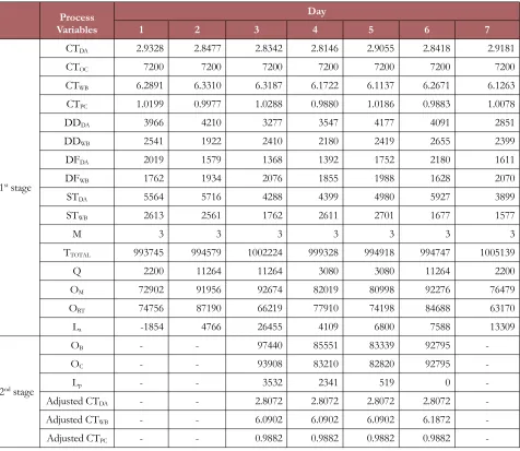
Case Study 3: Period 3
Table 4 shows the production planning data obtained for the 3rd period for 7 days.
Process Variables
Day
1 2 3 4 5 6 7
1st stage
CTDA 2.9328 2.8477 2.8342 2.8146 2.9055 2.8418 2.9181
CTOC 7200 7200 7200 7200 7200 7200 7200
CTWB 6.2891 6.3310 6.3187 6.1722 6.1137 6.2671 6.1263
CTPC 1.0199 0.9977 1.0288 0.9880 1.0186 0.9883 1.0078
DDDA 3966 4210 3277 3547 4177 4091 2851
DDWB 2541 1922 2410 2180 2419 2655 2399
DFDA 2019 1579 1368 1392 1752 2180 1611
DFWB 1762 1934 2076 1855 1988 1628 2070
STDA 5564 5716 4288 4399 4980 5927 3899
STWB 2613 2561 1762 2611 2701 1677 1577
M 3 3 3 3 3 3 3
TTOTAL 993745 994579 1002224 999328 994918 994747 1005139
Q 2200 11264 11264 3080 3080 11264 2200 OM 72902 91956 92674 82019 80998 92276 76479
ORT 74756 87190 66219 77910 74198 84688 63170
La -1854 4766 26455 4109 6800 7588 13309
2nd stage
OB - - 97440 85551 83339 92795
-OC - - 93908 83210 82820 92795
-Lp - - 3532 2341 519 0
-Adjusted CTDA - - 2.8072 2.8072 2.8072 2.8072
-Adjusted CTWB - - 6.0902 6.0902 6.0902 6.1872
-Adjusted CTPC - - 0.9882 0.9882 0.9882 0.9882
-Table 4. 1st Stage and 2nd Stage of Production Planning for 3rd Period
For day 1 in the 1st stage of production planning, O
in Table 1 and estimated OC(3) as 93908 units. Since OC(3) is lower than OB(3), there is a predicted throughput shortage that is required to be carried forward to the next day (i=4). Lp(3) is 3532 units.
For day 4, OM(4) is estimated at 82019 units. The predicted throughput shortage from day 3, Lp(3) are added to the planned throughput of day 4, OM(4). OB(4) is calculated as OM(4) + Lp(3) where it is equal to 85551 units. In the 2nd stage, the mathematical programming assessed the adjusted cycle time within the boundary shown in Table 1 and estimated OC(4) as 83210 units. When OC(4) is lower than OB(4), there is a predicted throughput shortage that is required to be carried forward to the next day (i=5). Lp(4) is 2341 units.
For day 5, OM(5) is estimated at 80998 units. The predicted throughput shortage from day 4, Lp(4) are added to the planned throughput of day 5, OM(5). OB(5) is calculated as OM(5) + Lp(4) where it is equal to 83339 units. In the 2nd stage, the mathematical programming assessed the adjusted cycle time within the boundary shown in Table 1 and estimated OC(5) as 82820 units. When OC(5) is lower than OB(5), there is a predicted throughput shortage that is required to be carried forward to the next day (i=6). Lp(5) is 519 units.
For day 6, OM(6) is estimated at 92276 units. The predicted throughput shortage from day 5, Lp(5) are added to the planned throughput of day 6, OM(6). OB(6) is calculated as OM(6) + Lp(5) where it is equal to 92795 units. In the 2nd stage, the mathematical programming assessed the adjusted cycle time within the boundary shown in Table 1 and estimated OC(6) as 92795 units compare. When OC(6) is equal to OB(6), there is no predicted throughput shortage that is required to be carried forward to the next day (i=7).
For day 7, OM(7) is estimated at 76479 units, and ORT(7) is 63170. Since OM(7) is higher than ORT(7), there is throughput shortage; thus the throughput shortage of day 7, (La(7)=13309 units) is carried forward to the 2nd stage of production planning for day 8. Since the case study is limited to seven days period, the analysis stops at this point.
5. The Implication of Throughput Shortage Recovery
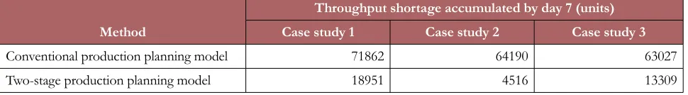
Table 5 shows the summary of losses data for each period.
Method
Throughput shortage accumulated by day 7 (units) Case study 1 Case study 2 Case study 3
Conventional production planning model 71862 64190 63027 Two-stage production planning model 18951 4516 13309
Table 5. Summary of losses data for Each Period
Table 2, Table 3, and Table 4 are essentially a simulation of the 2-stage of production planning to analyse throughput shortage occurrence. In the model, (OB-OC) is analogous to (OM-ORT). (OB-OC) reflects the condition of throughput shortage if the two-stage production planning model is adopted. Referring to Table 5, the model can reduce the accumulated throughput shortage incurred over a week, based on a comparison of throughput shortage from conventional method (summation of La over the 7 day period) and 2-stage of production planning model (La on day 7 if Lp on day 6 is zero or negative, or Lp on day 7 if Lp on day 7 is positive).
It is shown that adopting the two-stage production planning model can recover the throughput shortage, but the production capacity always limits the system based on the boundary of process parameters. However, when the real-time throughput is lower than the planned throughput, it is subjected to the throughput shortage recovery mode, causing parameters adjustment to recover the throughput shortage and meet the demand for subsequent day simultaneously. If the adjusted parameters are outside the boundary of process parameters, there is flexibility in production capacity to recover the throughput shortage completely. However, this area has not been explored, as the boundary of process parameters ensures that the quality of the product is not compromised.
2005). Hence the cycle time can fluctuate. In addition, the presence of product variety is reflected by the fluctuation of the cycle time which is also induced by the range of machine settings due to setup and batch variation.
If the throughput shortage is not carried forward in the subsequent day of planning, it will create a backlog of unprocessed batches, thus interrupting the production flow and causing a delay in meeting the demand and due date. Also, when there is no adjustment on the process parameters, there is a possibility that there will be an additional generation of throughput shortage since the throughput shortage may not be recovered with the original setting of the process parameters. In practice, when the WIP build-up is too high, the loading of machines can be stopped to reduce the unprocessed backlog. The proposed model suppresses the need to stop machine loading when WIP build-up is too high, as WIP build-up is mitigated through the cycle time adjustment.
The planned capacity in a single process pushes the maximum throughput available to next process. The relationship between throughput and process parameters is typically established in a production planning model for a single process. As the manufacturing system becomes more complex, the structural configuration that relates to the number of processes become crucial for the model. The reason for integrating processes in planning instead of individual processes is it enables overview planning of the system that manages the products flow from the first process to the last process. It also ensures that the planned throughput is met at the end of the system. Integrating throughput shortage in the subsequent day of planning requires an active relationship between process parameters of integrated processes and planned throughput. When the number of processes increases, the number of process parameters also increases. Thus, it is a challenge to model a large number of processes and process parameters to perform estimation effectively.
Adjustment of process parameters plays an essential role in enhancing the competitiveness of an assembly semiconductor manufacturing system to meet demand and recover the throughput shortage. It improves the responsiveness to real-time throughput and throughput shortage. Chen (2013) proposed a planned cycle time reduction using a systematic procedure. However, the study still lacks a clear relationship between the process parameters and throughput shortage. Macher and Mowery (2003) and Chien, Hsu and Hsiao (2012) stated that adjustment of process parameters affects the productivity change by realigning the desired level of throughput in the production line. Although the process parameters are crucial to throughput performance, existing studies did not express the association between adjustment of process parameters with throughput and throughput shortage in the production planning model. The novelty of the proposed production planning model is the throughput and throughput shortage can be manipulated through adjustment of process parameters. Process parameters are adjusted within an allowable range of values at the 2nd stage, which is essential to maintain the product quality during the production run and recover the throughput shortage. This is because the adjusted parameters within these settings control and sustains the process variation to avoid product quality deviation during the production run (Kao, 2010; Michaloski, Zhao, Lee & Rippey , 2013). Recurrence of product defect in such circumstances are caused by other factors such as tools wear and tear, quality of material, and other machine settings such as dispensing pressure, air pressure, or pattern recognition.
Indirectly, the cost of production improvement can be diverted to other activities since the process parameters can be adjusted with minimum cost. The significance of the framework is the establishment of a reference to develop the numerical relationship between process parameters with throughput and throughput shortage. Thus, it becomes feasible to adjust process parameters in multiple-process integration to plan for the future.
6. Conclusion
There are few areas to extend this research. First, the inclusion of additional parameters such as material and resource availability can further improve the model representation to the manufacturing system. Second, existing parameters such as downtime and set up time can be included to enhance the model flexibility in meeting demand and restore the throughput shortage simultaneously. Third, the framework reference can be further extended to more processes to test the repeatability and reproducibility of the approach. A large number of validations can further generalise the model effectiveness in different settings.
Declaration of Conflicting Interests
The authors declared no potential conflicts of interest with respect to the research, authorship, and/or publication of this article.
Funding
The authors acknowledge the YUTP-FRG grant (0153AA-E36) provided by Yayasan UTP for funding the study that resulted in publishing this article.
References
Anantharaman, N., & Nachiappan, R.M. (2006). Evaluation of Overall Line Effectiveness (OLE) in a Continuous Product Line Manufacturing System. Journal of Manufacturing Technology Management, 17(7), 987-1008.
https://doi.org/10.1108/17410380610688278
Chan, S.W., Tasmin, R., Aziati, A.H.N., Rasi, R.Z., Ismail, F.B., & Yaw, L.P. (2017). Factors Influencing the Effectiveness of Inventory Management in Manufacturing SMEs. IOP Conference Series: Materials Science and Engineering, 226(1). https://doi.org/10.1088/1757-899X/226/1/012024
Chen, T. (2013). A Systematic Cycle Time Reduction Procedure for Enhancing the Competitiveness and Sustainability of a Semiconductor Manufacturer. Sustainability (Switzerland), 5(11), 4637-4652.
https://doi.org/10.3390/su5114637
Chien, C.F., Hsu, C.Y., & Hsiao, C.W. (2012). Manufacturing Intelligence to Forecast and Reduce Semiconductor Cycle Time. Journal of Intelligent Manufacturing, 23(6), 2281-2294. https://doi.org/10.1007/s10845-011-0572-y
Enginarlar, E, Jingshan-Li, S.M.M., & Zhang, R.Q. (2002). Buffer Capacity for Accommodating Downtime in Serial Production Lines. International Journal of Production Research, 40(3), 601-624.
https://doi.org/10.1080/00207540110091703
Gandhi, A., & Harchol-Balter, M. (2009). M/G/K with Exponential Setup. School of Computer Science. Carnegie Mellon University.
Gram, M. (2013). A Systematic Methodology to Reduce Losses in Production with the Balanced Scorecard Approach. Manufacturing Science and Technology, 2(1), 12-22. https://doi.org/10.13189/mst.2013.010103
Hassani, L., & Hashemzadeh, G. (2015). The Impact of Overall Equipment Effectiveness on Production Losses in Moghan Cable & Wire Manufacturing. International Journal for Quality Research, 9(4), 565-576. Available at:
http://www.scopus.com/inward/record.url?eid=2-s2.0-84949643997&partnerID=tZOtx3y1
Kao, S.C. (2010). Deciding Optimal Specification Limits and Process Adjustments under Quality Loss Function and Process Capability Indices. International Journal of Industrial Engineering : Theory Applications and Practice , 17(3), 212-222.
Khan. (2007). Industrial Engineering. New Age International.
Macher, J.T., & Mowery, D.C. (2003). Managing” Learning by Doing: An Empirical Study in Semiconductor Manufacturing. Journal of Product Innovation Management, 20(5), 391-410. https://doi.org/10.1111/1540-5885.00036
Miltenburg, J. (2000). The Effect of Breakdowns on U-shaped Production Lines. International Journal of Production Economics, 58(2), 183-189. https://doi.org/10.1080/002075400189455
Nemtajela, N., & Mbohwa, C. (2017). Relationship between Inventory Management and Uncertain Demand for Fast Moving Consumer Goods Organisations. Procedia Manufacturing, 8(October), 699-706.
https://doi.org/10.1016/j.promfg.2017.02.090
Pinedo, M.L. (2005). Planning and Scheduling in Manufacturing and Services. Springer. United State of America.
https://doi.org/10.1017/CBO9781107415324.004
Prajapati, M., & Deshpande, V. (2015). Cycle Time Reduction using Lean Principles and Techniques : A Review.
Journal, International Engineering, Industrial, 3(December).
Salameh, M.K., & Ghattas, R.E. (2001). Optimal Just-In-Time Buffer Inventory for Regular Preventive Maintenance. International Journal of Production Economics, 74(1–3), 157-161. https://doi.org/10.1016/S0925-5273(01)00122-0
Sana, S.S., & Chaudhuri, K.S. (2010). An EMQ Model in an Imperfect Production Process. International Journal of System Science, 41(6), 635-646. https://doi.org/10.1080/00207720903144495
Sana, S.S. (2012). Preventive Maintenance and Optimal Buffer Inventory for Products Sold with Warranty in an Imperfect Production System. International Journal of Production Research, 50(23), 6763-6774.
https://doi.org/10.1080/00207543.2011.623838
Sharma, P., & Jain, A. (2015). Stochastic Dynamic Job Shop Scheduling with Sequence-Dependent Setup Times: Simulation Experimentation. Journal of Engineering and Technology, 5(1), 19. https://doi.org/10.4103/0976-8580.149475
Siva, R., Patan, M.N.K., Kumar, M.L.P., Purusothaman, M., Pitchai, S.A., & Jegathish, Y. (2017). Process Improvement by Cycle Time Reduction through Lean Methodology. IOP Conference Series: Materials Science and Engineering, 197(1). https://doi.org/10.1088/1757-899X/197/1/012064
Salvendry, G. (2007). Handbook of Industrial Engineering: Technology and Operations Management (3rd ed.). Wiley Online Library. https://doi.org/10.1002/9780470172339
Tekin, İ., & Sıtkı, G. (2012). Determination of Costs Resulting from Manufacturing Losses : An Investigation in White Durables Industry. Proceedings of the 2012 International Conference on Industrial Engineering and Operations Management Istanbul, Turkey, 352-361.
Telsang, M. (2010). Industrial Engineering and Production Management. S. Chand and Company LTD, New Delhi. Wuest, T., Weimer, D., Irgens, C., & Thoben, K.D. (2016). Machine Learning in Manufacturing: Advantages,
Challenges, and Applications. Production & Manufacturing Research, 4(1), 23–45.
https://doi.org/10.1080/21693277.2016.1192517
Xu, X., Zhao, Y., Wu, M., Zhou, Z., Ma, Y., & Liu, Y. (2016). Stochastic Customer Order Scheduling to Minimize Long-Run Expected Order Cycle Time. Annals of Operations Research, 7543(September), 1-24.
https://doi.org/10.1007/s10479-016-2254-9
Zequeira, R.I, Prida, B., & Valdes, J.E. (2004). Optimal Buffer Inventory and Preventive Maintenance for an Imperfect Production Process. International Journal of Production Research, 42(4), 959-974.
https://doi.org/10.1080/00207540310001631610
Journal of Industrial Engineering and Management, 2019 (www.jiem.org)
Article’s contents are provided on an Attribution-Non Commercial 4.0 Creative commons International License. Readers are allowed to copy, distribute and communicate article’s contents, provided the author’s and Journal of Industrial Engineering and