A unifying process capability metric

(1)

doi:10.3926/jiem.2009.v2n1.p48-59 ©© JIEM, 2009 – 2(1): 48-59 – ISSN: 2013-0953

A unifying process capability metric

John Jay Flaig

Applied Technology (USA)

[email protected]

Received December 2008 Accepted April 2009

Abstract:

A new economic approach to process capability assessment is presented, which

differs from the commonly used engineering metrics. The proposed metric consists of two

economic capability measures – the expected profit and the variation in profit of the

process. This dual economic metric offers a number of significant advantages over other

engineering or economic metrics used in process capability analysis. First, it is easy to

understand and communicate. Second, it is based on a measure of total system

performance. Third, it unifies the fraction nonconforming approach and the expected loss

approach. Fourth, it reflects the underlying interest of management in knowing the

expected financial performance of a process and its potential variation.

Keywords:

process capability, profitability, variation in profit

1 Introduction

(2)

process capability – profitability. Thus, the new metric should significantly help improve the bottom line financial results of companies that choose to adopt it.

In the recent survey article on Process Capability Indices, by Kotz and Johnson, several discussants suggested that a single metric is insufficient to adequately describe process capability and that multiple metrics are required (Kotz, 2002) (Bothe, 2002). Further, Hubele (2002) and Ramberg (2002) suggest that whatever capability metrics are proposed they should express both the expected value of the metric and an estimate of its variation. The author agrees with both of these suggestions, so the ordered pair notation, CM = [E(M), SD(M)] will be used, where

M denotes the metric, CM denotes the M-capability metric, E(M) is the expected

value of the metric, and SD(M) is the standard deviation of the metric. For additional background on process capability measurement the reader is referred to the text by Pearn and Kotz (Pearn, 2006), or the book by Bothe (Bothe, 2001).

As most practitioners are aware statisticians view all of the commonly used capability indices (i.e., Cp, Cpk, Cpm, and fraction nonconforming (NC)) with various degrees of concern. Hence, numerous “better” alternatives have been proposed (more than 100 at last count). There has been great deal of research in the area of engineering process capability metrics but very little on economic metrics and almost none on dual economic metrics for assessing process capability. One of the more recent economic proposals is to use the quadratic expected loss as a capability metric. However, there are concerns with this metric also which will be discussed next.

2 The loss metric

Some authors (Spiring, 2002; Ramberg, 2002) have proposed using the economic expected loss metric (EL) as a capability measure. This metric has the advantage that it reflects the more modern and reasonable quality loss philosophy rather than the classic binary cost model (used in the fraction nonconforming metric NC). Thus, the expected loss might be a good choice for a metric, if it mapped seamlessly into the underlying concept of capability.

(3)

management. Thus, from a management and communication point of view, it is not a sufficient statistic from which to infer the capability of the process. The source of the problem, in the author’s opinion, is that the expected loss metric focuses only on costs and this is not a sufficient basis for a metric that is supposed to span the space of interests of all concerned in assessing process capability. To understand why a cost based model of capability does not provide sufficient information it is necessary to consider the entire production process as a system. This is the focus of the next section.

3 The cost fallacy

One of the classic concerns of process improvement is how to minimize cost, the assumption being that this will lead to increased profitability. Intuitively this seems like a reasonable assumption, but is it a valid assumption? The answer unfortunately is no. As Liebhold (2001) points out:

One major point has been overlooked in most quality engineering publications: the overriding goal of companies within an industry is the maximization of profit to allow for reinvestment and further growth and profits. Indeed, whereas most research focuses on quality improvement and its related cost, it does not take into account the impact of quality on quantities sold and the sale price. Because the survival and development of a company depends on profit generation, reduction in costs is useless if it is not compared to its direct impact on revenues.

(4)

4 The profit metric

This approach to process capability assessment can be applied to any enterprise that produces a product for a profit. The business model below assumes that all units are inspected before shipping, and inspection is 100% effective (i.e., there is no measurement system error), and that all units produced during the period are sold (i.e., no inventory accumulation). It is assumed that this analysis is for a stable process and at a fixed point on the products supply and demand curve.

The business performance metric used in this paper is defined to be:

Gross Profit = Net Sales Revenue – Cost of Goods Sold (1)

On a “per unit” basis equation 1 becomes:

Gross Profit per Unit (GPPU) = [RPU x (Process Yield)] – [COGS per Unit] (2)

where RPU is the revenue per unit (assumed constant under the assumptions given above).

COGS is the Cost of Goods Sold and is given by:

COGS = [Beginning Inventory + Cost of Product Produced – Ending Inventory]

Assuming that beginning and ending inventories are equal, then equation 2 becomes:

GPPU = [RPU (Process Yield)] – [Cost of Product Produced per Unit] (3)

Let x be the measurement of a Quality characteristic of interest on a unit. A unit is defined as nonconforming (NC) if x > Upper Spec Limit (USL) or x < Lower Spec Limit (LSL). If NC is the process fraction nonconforming, then 1 – NC is the process yield. Further, the cost of product per unit, CPPU, is given by:

CPPU = CL + CM + CE + CF + CO (4)

where CL is the cost of labor, CM is the cost of materials, CE is the cost of

equipment, CF is the cost of product failure, and CO is all other production costs. In

(5)

The gross profit per unit is then given by:

GPPU = [RPU (1 – NC)] – [CL + CM + CE + CF + CO] (5)

If operating costs (i.e., sales and marketing, and general and administrative) were included, then equation 5 would reflect net profit rather than gross profit.

There are three approaches to estimation of the product failure cost CF. They are

quality cost, process cost, and quality loss (Campanella, 1999). The quality loss approach characterized by the Taguchi quadratic expected loss per unit function (EL) will be used in this paper to estimate CF.

Replacing CF in equation 5 with EL yields:

GPPU = [RPU (1 – NC)] – [CL + CM + CE + CO+ EL] (6)

The proposed dual economic process capability metric for gross profit is defined to be:

CGP = [E(GPPU), SD(GPPU)], or more simply [E(GP), SD(GP)] (7)

Assuming our company produces a product that has a stable quality characteristic distribution (not necessarily Normal) having mean  standard deviation  with a fixed process target T and constant specification limits (LSL, USL), then the quadratic expected loss is given by EL = c (2_{+ (}__{– T)}2_{), where c is the constant}

estimated economic loss per unit, and T is the process target. So the first term, E(GP), in the CGP metric is given by:

E(GP) = [RPU (1 – E(NC))] – [CL + CM + CE + CO + c E(s2 + (m – T)2)] (8)

where m is the arithmetic mean, and s is the Root Mean Square (RMS) standard deviation. Thus NC and EL are functions of the random variables m and s, which are estimates of the population parameters  and  respectively. The functional form of NC is not specified but can be approximated by modeling the process distribution (Farnum, 1996; Flaig, 2002) or empirically by periodic sampling of the process.

The second term in our dual CGP metric, SD(GP), must still be determined. So

(6)

V(GP) = V([RPU (1 – NC)] – [CL + CM + CE + CO + EL]) (9)

Since RPU, CL, CM, CE, and CO are constants, and NC and EL are functions of m and

s, then distributing the variance operator over equation 9 yields:

V(GP) = V(– RPU NC)) + V(– EL) + 2(–RPU)(–1) Cov(NC, EL) (10)

= RPU2_{V(NC) + V(EL) + 2 RPU Cov(NC, EL)}

where Cov(NC, EL) = (NC, EL) SD(NC) SD(EL)

If sufficient daily or weekly production data are available from a stable process, then all the terms in E(GP) and V(GP) can be estimated by periodic sampling of the process data. That is, the practitioner could estimate the correlation coefficient

(NC, EL) and other terms with a known degree of confidence and hence provide an estimate of CGP. However, the terms in equation 10 may be further simplified for

computation purposes by finding V(EL) and V(NC).

Since c is a constant, and m and s are random variables, it follows that EL is a random variable. So taking the variance of the expected loss function yields:

V(EL) = V(c(s2_{+ (m – T)}2₎₎ ₍₁₁₎

= c2_[V(s2_{+ (m – T)}2_)]

= c2_[V(s2_{) + V((m – T)}2_{) + 2Cov(s}2_{, (m – T)}2_)]₍₁₂₎

Further, since s is the RMS standard deviation, then equation 12 can be expanded as follows:

V(s2_{) =}

E(s4)E2(s2) 42 2

n ,wherer1 /n (xm) r

i1 n



and

V((m – T)2_{) =}

E((mT)4)E2((mT)2) ₁4 ₁4 0,where_r1 /n (xT)r

i1 n



(7)

Cov(s2_{, (m – T)}2_{) =}__(s2_{, (m – T)}2_{) SD(s}2_{) SD((m – T)}2₎

= (s2_{, (m – T)}2₎

422

n 0 = 0

Thus,

V(EL) = c2₍

422

n + 0 + 2 (s

2_{, (m – T)}2₎

₄₂2

n 0) = c

2₍

422

n ) (13)

All that remains to be done is to determine the standard deviation of the fraction nonconformance, SD(NC). The variance of NC is given by:

V(NC) = NC (1–NC)/n, from which it follows that,

SD(NC) = [(NC (1–NC))/n]1/2 ₍₁₄₎

Thus, the standard deviation of gross profit, GP, is given by:

SD(GP) = [RPU2_{V(NC) + V(EL) + 2 RPU}__{(NC, EL) SD(NC) SD(EL)]}1/2 ₍₁₅₎

Combining the two performance measures E(GP) and SD(GP) to form the gross profit capability metric CGP = [E(GP), SD(GP)] gives the practitioner a measure of

process capability that is directly connected to a concrete measure of financial performance and one that management is keenly interested in knowing.

5 A real world example

The dual response process capability optimization technique was discussed in a previous paper (Flaig, 2002) and the same technique will be used in this example. However, in this case the goal is to optimize CGP in the sense of maximizing the

expected profit, E(GP), and simultaneously minimizing the variation in profit, SD(GP), to achieve the most economically capable process. However, since these dual objectives sometimes conflict the practitioner must decide on an optimization approach. There are several approaches to dual response optimization (Copeland, 1996; Del Castillo, 1993), but the profit signal-to-noise ratio (i.e., SN(GP) = E(GP)/SD(GP)) will be used in this paper.

(8)

 An economic model of the process (i.e., a business model).

 A process model (i.e., an adequate model of a stable process)

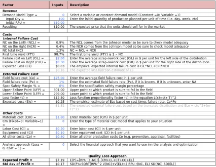
Now, consider the following real world example of a pipe grinding operation (Trietsch, 1997). As noted the inputs are required for the analysis are a business model and a process model. Below is a business model for the pipe grinding operation (values not given by Trietsch are provided by the author and are based on typical values observed in industry).

Factor Inputs Description Revenue

Demand Model Type = 0 Select a variable or constant demand model (Constant =0; Variable =1)

Input Qty = 100 Enter the initial quantity of production planned per unit of time (i.e. day, week, etc) Initial RPU = $10.00

Resulting $10.00 The expected price that the units should sell for in the market

Costs

Internal Failure Cost

NC on the Leith (NCL) = 0.9% The NCL comes from the Johnson model so be sure to check model adequacy NC on the right (NCR) = 0.4% The NCR comes from the Johnson model so be sure to check model adequacy NC total (NC) 1.3% NC = NCL + NCR

First time yield (FTY) 98.7% The first time yield (FTY) is 1 – NC

Failure cost on Left (CiL) = $2.60 Enter the average scrap-rework cost (CiL) in $ per unit for the left side of the distribution Failure cost on Right (CiR) = $0.30 Enter the average scrap-rework cost (CiR) in $ per unit for the right side of the distribution Expected Loss (Eli) $0.03 The empirical expected internal failure cost is CiL*NCL+CiR*NCR

$0.16 The expected loss function estimate of Eli

External Failure Cost

Field failure cost (Ce) = $25.00 Enter the average field failure cost in $ per unit

Field failure rate (Pe) = 1% Enter the estimated field failure rate (Pe), if it is known. If it is unknown, enter NA Spec Safety Margin % = 0% Enter the specification safety margin percentage

Upper Failure Point (UFP) = 301.00 Upper point at which product is sure to fail in the field Lower Failure Point (LFP) = 299.00 Lower point at which product is sure to fail in the field

Loss factor (c) = $12.50 Loss function proportionality factor (c) in the equation L(x)=c(x-T)^2 Expected Loss (Ele) = $0.25 The empirical estimate of ELe based on cost times failure rate, Ce*Pe

$1.81 The expected external failure cost based on the truncated distribution and ELe = c(s^2+(m-T)^2)

Other Costs

Materials cost (Cm) = $1.80 Enter material cost (Cm) in $ per unit Cm (Fixed=0; Variable=1)

= 0 Enter the type of material cost model that applies to your situation Labor Cost (Cl) = $0.20 Enter labor cost (Cl) in $ per unit

Equipment cost (Ct) $0.10 Enter equipment cost (Ct) in $ per unit

All other costs (Co) = $0.40 Enter all other production costs Co (e.g. prevention, appraisal, facilities) Analysis approach (Loss =

0, Cost = 1) = 0 Select the financial approach that you want to use inn the analysis and optimization

Quality Loss Approach Expected Profit = $7.19 E(P)=[RPU (1-NC)]-[CM+CL+CT+CO+EL]

Std dev of Profit = $0.17 SD(P)=SQRT[RPU^2 V(NC)+V(EL)+2 RPU r(NC, EL) SD(NC) SD(EL)]

Table 1. “Pipe Grinding Business Model”.

It should be noted that for the CGP maximization approach to yield reasonable

(9)

optimization model are dx and k, where dx is process mean shift and k is the process sigma multiplier, and the output variable is the profit signal to noise ratio SN(GP). From this information it is possible to evaluate the expected performance of the process in its initial state.

Objectives Description Weights (Wi) Results

NC  0 Minimize the fraction nonconforming 1 13,467

NS  0 Minimize the sensitivity to variation 1 23,843

DT  0 Minimize the deviation from target 1 -0.02

S  0 Minimize the process variation 0.3966

Expected (Profit)  Infinity Maximize profit 1 $7.19

Std Dev (Profit)  0 Minimize profit variation 1 $0.09

Table 2. “Expected performance of the process in its initial state”.

Since the original observed data was not available, the performance of the pipe grinding operation was simulated based of the parameters given (i.e., 1,000 values were drawn at random from N(300, 0.4)) with the following results:

The process in its initial state (i.e., dx = 0, k = 1) has capability CGP = [$7.19, $0.09] and Cpk = 0.82.

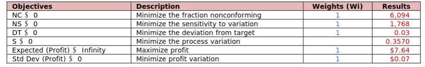
Now suppose experiments were performed that resulted in a 10% reduction in variation, then adjusting the mean shift (dx) and sigma multiplier (k) inputs to achieve profit signal-to-noise maximization results in the following:

Objectives Description Weights (Wi) Results

NC  0 Minimize the fraction nonconforming 1 6,094

NS  0 Minimize the sensitivity to variation 1 1,768

DT  0 Minimize the deviation from target 1 0.03

S  0 Minimize the process variation 0.3570

Expected (Profit)  Infinity Maximize profit 1 $7.64

Std Dev (Profit)  0 Minimize profit variation 1 $0.07

Table 3. “Expected performance of the process with a 10% reduction in variation”.

when the inputs are set to dx = 0.05, and k = 0.90. The adjusted process has capability under these conditions of CGP = [$7.64, $0.07] and Cpk = 0.91.

If these operating conditions could be achieved, then the expected fraction nonconforming would be reduced by 7,375 defectives per million (45%), profits would increase by $0.45 (6%), and the standard deviation of profits would decrease by $0.02 (22%). As illustrated in this example, using the CGP metric for

(10)

6 Conclusions

As the example shows the use of the profit metric CGP = [E(GP), SD(GP)] has

significant advantages over Cpk in driving process improvement. Similarly, it can be shown that it also offers advantages over other capability metrics such as Cp, Cpm, Cpmk, NC, or dual metrics such as CNC = [NC, NS], and the expected loss

metric CEL = [E(EL), SD(EL)] because:

1. The profit metric CGP focuses on bottom line issues -- profit and profit variation

rather than components of production system performance such as costs, the ratio of specification width to process width, or fraction nonconforming rates.

2. The profit metric CGP does not mislead management into adopting operating

conditions that may actually sub-optimize profitability as some other capability indices such as Cpk and Cpm can (Flaig, 2002). This fact alone constitutes a major change in the area of process optimization practice as many people now follow the Six Sigma methodology of using Cpk as the process optimization metric.

3. The profit metric CGP includes both NC and EL as input variables so it offers an

approach that unifies these two contending process capability analysis philosophies. Clearly, the nonconformance rate and the expected loss are both important components in any reasonable view of what constitutes process capability. Hence, rather than arguing that one is better than the other the CGP

metric incorporates the value of both. Thus providing a unification of the concepts and making the controversy mute.

4. The profit metric CGP focuses on two key financial indices by which all processes

are judged – expected profit and the stability of profit generation. Thus, it provides an excellent process performance communication tool, and one that has a good chance of being implemented by management.

There are a vast number of process capability metrics to choose from, many of which are complex, non-intuitive, and hard to understand and communicate. Asking people to adopt a new metric requires that it fulfill an unmet need and be superior to other capability metrics in each of the areas listed above to have any chance of implementation. The only metric that seems to meet these requirements and fulfill management’s unmet need for a systematic capability measure is the CGP

(11)

References

Bothe, D. R. (2001). Measuring Process Capability. Landmark Publishing, Inc., Cedarburg, WI.

Bothe, D. R. (2002). PCI Discussion. Journal of Quality Technology, 34(1), 32-37.

Campanella, J. et. al. (1999). Principles of Quality Costs. ASQ Quality Press, Milwaukee, WI.

Copeland, K. A. F., & Nelson, P. R. (1996). Dual Response Optimization via Direct Function Minimization. Journal of Quality Technology, 28(3), 331-336.

Del Castillo, E., & Montgomery D. C. (1993). A Nonlinear Programming Solution to the Dual Response Problem. Journal of Quality Technology, Vol. 25, No. 3, pp. 199-204.

Farnum, N. R. (1996). Using Johnson Curves to Describe Non-normal Process Data. Quality

Flaig, J. J. (1999). Process Capability Sensitivity Analysis. Quality Engineering, Marcel Dekker, 11(4), 587-592.

Flaig, J. J. (2002). Process Capability Optimization. Quality Engineering, Marcel Dekker, 15(2), 233-242.

Hubele, N. F. (2002). PCI Discussion. Journal of Quality Technology, 34(1), 20-22.

Liebhold, V. S., Kimbler, D. L., & Gramopadhye, A. K. (2001). A Profit-Based Model Allowing for Quality Achievement and Manufacturing Process Selection. Quality Engineering, Marcel Dekker, 14(1), 25-32.

Leland, H. E. (1972). Theory of the Firm Facing Uncertain Demand. American Economic Review, 62(3), 278-291.

Lau, H.-L.A., & Lau H. S. (1988). The Newsboy Problem with Price Dependent Demand Distribution. IIIE Transactions, 10, 409-415.

(12)

doi:10 Pear Pro 216 Pear Ind Ram 50 Spiri Qu Triet Adj a Engine 0.3926/jiem.2

n, W. L., operties of

6-231.

n, W. L., & dices. World

berg, J. S. .

ng, F., Che uality Techn

tsch, D. (1 justment P

Article's conte allowed to copy,

eering and Man

2009.v2n1.p48

Kotz, S., Process C

& Kotz, S. d Scientific

. (2002). P

eng, S., Ye nology, 34(

1997). The rocedure. Q

©© Journal o

ents are provide , distribute and

agement's nam license content

8-59

& Johnson Capability I

(2006). En Publishing

PCI Discuss

eung, A., & 1), 23-27.

e Five/Ten Quality Eng

of Industrial Eng

ed on a Attributi communicate a mes are included ts, please visit h

©©

n, N. L. (1 Indices. Jo

ncyclopedia Company,

sion. Journa

& Leung, B

Rule: A gineering, M

gineering and M

on-Non Comme rticle's contents d. It must not be http://creativeco

JIEM, 2009 –

1992). Dist urnal of Q

and Handb , Vol. 12.

al of Quali

B. (2002).

Constraine Marcel Dekk

Management, 20

ercial 3.0 Creati s, provided the a e used for comm mmons.org/lice

– 2(1): 48-59

tributional Quality Tech

book of Pro

ty Technolo

PCI Discus

ed-Loss Eco ker, 10(1),

009 (www.jiem.o

ve commons lic author's and Jou mercial purposes nses/by-nc/3.0/

– ISSN: 2013

and Infere hnology, 2

ocess Capa

ogy, 34(1)

sion. Journ

onomic Pro 85-95.

org)