A deterministic algorithm for generating optimal three-stage layouts of homogenous strip pieces

JIEM, 2014 – 7(5): 1167-1182 – Online ISSN: 2013-0953 – Print ISSN: 2013-8423 http://dx. doi. org/10. 3926/jiem. 1127

A

D

eterministic

A

lgorithm for

G

enerating

O

ptimal

T

hree-S

tage

layouts of

H

omogenous

S

trip

P

ieces

Jun Ji

1

, Fei-Fei Xing

2

, Jun Du

1

, Ning Shi

1

, Yao-Dong Cui

3

1

Beijing Polytechnic (China)

2

BMEI CO., LTD. (China)

3

Guangxi University (China)

[email protected], [email protected], [email protected], [email protected], [email protected]

Received: March 2014

Accepted: September 2014

Abstract:

Purpose:

The time required by the algorithms for general layouts to solve the large-scale

two-dimensional cutting problems may become unaffordable. So this paper presents an exact

algorithm to solve above problems.

Design/methodology/approach:

The algorithm uses the dynamic programming algorithm

to generate the optimal homogenous strips, solves the knapsack problem to determine the

optimal layout of the homogenous strip in the composite strip and the composite strip in the

segment, and optimally selects the enumerated segments to compose the three-stage layout.

Findings:

The algorithm not only meets the shearing and punching process need, but also

achieves good results within reasonable time.

are better than that of the above three algorithms. Experimental results show that the algorithm

to solve a large-scale piece packing quickly and efficiency.

Keywords:

two-dimensional layout, homogenous strip, dynamic programming recursion

1. Introduction

The unconstrained two-dimensional cutting (UTDC) problem refers to a series of small shape (or part) non-overlapping on a rectangular panel and the optimization objective of the problems is to find an arrangement for maximizing the material usage. UTDC problem is widely used in the leather, wood, metal and other manufacturing industries. Although many researchers have studied the UTDC problem, from the theory of computational complexity theory, layout problem have been proved to be a quiet difficult combinatorial optimization problem (Cui, 2013; Han, Bennell & Zhao, 2013; Thomas & Chaudhari, 2013; He & Wu, 2013; Liu & Liu, 2011; Ji, Lu & Cha, 2012; Huang & Liu, 2006; Jiang, Lv & Liu, 2008).

According to the UTDC problem, the layouts can be divided into the general layouts and the specific layouts. On the one hand, when the layouts have no any constraint, the layouts are called the general layouts (Gilmore & Gomory, 1965; Beasley, 1985; Cui, Wang & Li, 2005; Seong & Kang, 2003; Hifi & Zissimopoulos, 1996; Alvarez-Valdes, Parajon & Tamarit, 2002); on the other hand, when the layouts must meet some specific production request, the layouts are called the specific layout.

Now, there are some exact algorithms for the general layouts (Gilmore & Gomory, 1965; Cui et al., 2005). But the computation results in the references indicate that the computation time of these algorithms cannot be intolerable for solving the large scale UTDC problems. So many researchers have committed to study the specific layouts. The specific layouts have three advantages: meeting the practical production technology; high computation efficiency; the results are close to the optimal results.

3HS layout is the superset of the classic three-stage, two-segment, T-shape and the classic two-stage layout, and we will introduce it in the section 2.4.

The layout decides the layout value. The sequence of the above layouts value from largest to smallest is follows: the general layout, the classic three-stage layout, the two-segment layout, the T-shape layout, and the classic two-stage layout. This paper’s 3HS layout is between the general layout and the classic three-stage layout.

This paper will introduce 3HS layout in part 2; the exact algorithm for generating the 3HS layout in part 3; the experiments and results analysis in part 4; conclusion in part 5.

2. 3HS layout

2.1. Homogenous stripe

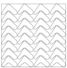
The homogenous stripe consists of the same size with same dimension. Figure 1(a) shows horizontal homogenous rectangular stripes, and its width is the blank width. Figure 1(b) shows vertical homogenous irregular stripes, and its width is the blank length.

(a) The horizontal homogenous stripe (b) The vertical homogenous stripe

Figure 1. The homogenous stripe

2.2. Composite strip

(a) The X composite strip (b) The Y composite strip

Figure 2. The composite strip

Figure 3 shows the process of its being cut. The arrow is the cut station, and the number is the cuts sequence. After the composite strip cut into homogenous stripe, the blank is been separated from homogenous stripe by the punch.

Figure 3. The cutting process of composite strip

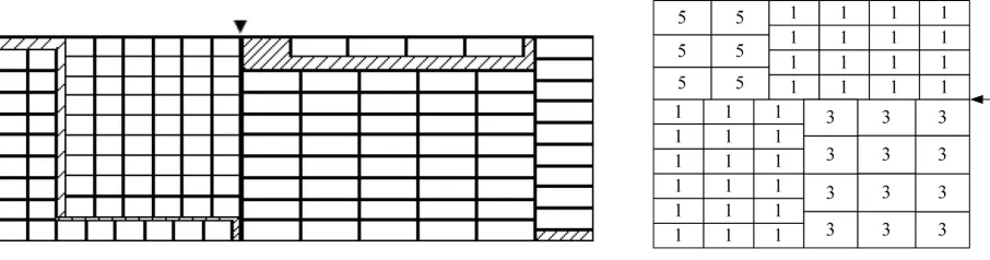
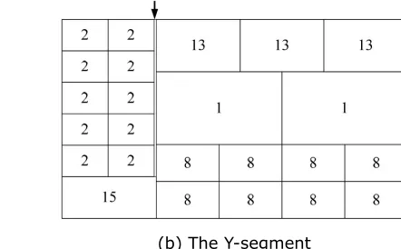
2.3. Segment

(a) The X-segment (b) The Y-segment

Figure 4. The segment

2.4. 3HS layout

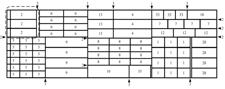
Figure 5 shows the 3HS layouts. Each 3HS layout composes of many segments. In 3HS layout, if it consists of some horizontal X-segments from left to right, it is called 3HSX layout (Figure 5(a)); if it consists of some vertical Y-segments from up to bottom, it is called 3HSY layout (Figure 5(b)).

(a) The 3HSX layout (b) The 3HSY layout

Figure 5. The types of the 3HS layout

Figure 6. The 3HSX layout and its cutting process

In 3HS layout, if each blank takes place of the homogenous strip, the 3HS layout turns into the classic three-stage layout; if the number of the segment is 2, the 3HS layout becomes the two-segment layout; if segments are X-segment and Y-segment, the 3HS layout turns into the T-shape layout. In addition, the T-shape layout is the superset of the classic two-stage layout (Cui, 2004a). Thus, the 3HS layout is the superset of the classic three-stage, two-segment, T-shape, and the classic two-stage layout. In other words, the solution of 3HS layout is better than that of the above four layouts.

3. The algorithm for generating 3HS layout

3.1. Notes and functions

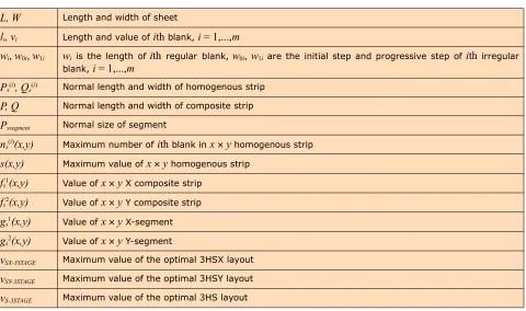
L, W Length and width of sheet

li, vi Length and value of ith blank, i = 1,...,m

wi, w0i, w1i wi is the length of ith regular blank, w0i, w1i are the initial step and progressive step of ith irregular

blank, i = 1,...,m

Ps(i), Qs(i) Normal length and width of homogenous strip P, Q Normal length and width of composite strip

Pssegment Normal size of segment

ns(i)(x,y) Maximum number of ith blank in x  y homogenous strip s(x,y) Maximum value of x  y homogenous strip

fs1(x,y) Value of x  y X composite strip fs2(x,y) Value of x  y Y composite strip gs1(x,y) Value of x  y X-segment gs2(x,y) Value of x  y Y-segment

vSX-3STAGE Maximum value of the optimal 3HSX layout

vSY-3STAGE Maximum value of the optimal 3HSY layout

vS-3STAGE Maximum value of the optimal 3HS layout

Table 1. Notes and function

3.2. The steps of algorithm

Supposed the size of sheet and blank are integer, and the blank direction is fixed. The algorithm of 3HS layout (3HSA) includes the following steps:

Step 1. Determining the optimal homogenous strip by dynamic programming algorithm;

Step 2. Solving the optimal homogenous strip layout in composite strip by knapsack problem;

Step 3. Solving the optimal composite strip in segment by knapsack problem;

Step 4. Determining the optimal 3HSX layout by knapsack problem;

Step 5. Determining the optimal 3HSY layout by knapsack problem;

Step 6. Solving the optimal 3HS layout.

3.3. The normal size

and

x0

is the optimal normal size that is lessen than

x

, and

y0

is the optimal normal size that is lessen than

y

. To different layout, according to normal size features, we should define it appropriately to improve the solving speed.

Definition 1. The homogenous strip normal size

According to above description, the homogenous strip consists of blanks with same shape, and the blank direction is fixed. Therefore, the homogenous strip length normal size

Ps

(i) _{is the}

length linear combination of each blank. The equation is follows:

(1) (1) The homogenous width normal size of regular blank

Qs

(i) _{is follows:}

(2) (2) The homogenous width normal size of irregular blank

Qs

(i) _{is follows:}

(3) The

0

and

L

are added to the normal size sequence. The

Ps

(i)

=

p1

s

,

p2

s

,...,

pM

s _{represents the}

homogenous strip length normal size of

i

th

blank, and

M

is the number of normal size; and the

Qs

(i)

=

q1

s

,

q2

s

,...,

qN

s _{represents the homogenous strip width normal size of}

i

th

_{blank, and}

N

_is

the number of normal size.

Definition 2. The composite strip normal size

According to above description, the composite strip composes of homogenous strips. So, the composite strip length normal size

P

is the length linear combination of each blank:

(4)

(1) The composite strip width normal size of regular blank

Q

is follows:

(2) The composite strip width normal size of irregular blank

Q

is follows:

(6)

The

0

and

L

are added to the normal size sequence. The

p1

,

p2

,...,

p

M represents the composite

strip length normal size, and

M

is the number of normal size; the

q1

,

q2

,...,

q

N represents the

composite strip width normal size, and

N

is the number of normal size.

Definition 3. The segment normal size

According to above description, the segment consists of composite strip. Therefore, the segment normal width

Pssegment

is the collection of composite strip length normal size:

(7) If both the segment width and length belong to

Pssegment

, then the segment is a normal segment.

3.4. The value of homogenous strip

x



y

(1) Solving the maximum number that the homogenous strip

x



y

includes blanks

Assume that

ns

(i)

(x, y)

_{is the maximum number of}

i

th

_{blank in the homogenous}

x



y

_{, and there}

is following recursive formula, and

x



Ps

(i)

,

y



Qs

(i):

• The maximum number of

i

th

regular blank in the homogenous

x



y

:

(8)

• The maximum number of

i

th

irregular blank in the homogenous

x



y

:

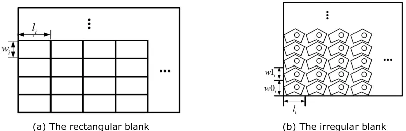
(a) The rectangular blank (b) The irregular blank

Figure 7. The blanks number of the homogenous strip x  y

(2) Determining the blank maximum value in homogenous

x



y

Suppose

s

(

x, y

)

is the maximum value in homogenous

x



y

, and

vi

is the

i

th

blank value, then:

(10)

3.5. Determining the homogenous strip optimal layout in composite strip

(1) Determining the homogenous strip optimal layout in X composite strip Suppose

fs

1

(

x, y

)

_{is the value of X composite strip}

x



y

_{, and}

x



P; y



Q

_:

(11)

The solution of above knapsack problem can refer to literature (Kellerer, Pferschy & Pisinger, 2004).

(2) Determining the composite strip optimal layout in Y composite strip Suppose

fs

2

(

x, y

)

_{is the value of Y composite strip}

x



y

_{, and}

x



P; y



Q

_:

3.6. Determining the section optimal layout in segment

Assume that

gs

1

(

x, y

)

_{is the value of X-segment}

x



y

, and

gs

2

(

x, y

)

is the value of Y-segment

x



y

. So, there is following formula, and

x, y



Pssegment

:

(13)

The following equation determines

gs

2

(

x, y

)

_:

(14)

3.7. The optimal 3HS layout

Suppose

vSX-3STAGE

is the value of optimal 3HSX layout:

(15)

Suppose

vSY-3STAGE

is the value of optimal 3HSY layout:

(16)

Suppose

vS-3STAGE

is the value of optimal 3HS layout:

(17)

3.8. The steps of generating the optimal 3HS layout

The algorithm for contains the following steps:

Step 1. Determining the normal of homogenous strip, composite strip and segment from Sect. 3.3.

Step 2. Determining the optimal homogenous strip from Sect. 3.4.

Step 3. Determining the optimal composite strip by equations (11) and (12).

Step 4. Determining the optimal segment by equations (13) and (14).

3.9. The time complexity of the 3HSA

The time it takes for determining the normal size of composite strip and section from Sect. 3.3 is

O

(

mL

)

.

The time it takes for determining the optimal homogenous strip from Sect. 3.4 is

O

(

mLW

)

. The time it takes for determining the optimal composite strip with equation (11) and (12) is

O

(

LW

2

+

WL

2

)

_.

The time it takes for determining the optimal segment with equation (13) and (14) is

O

(

L

2

+

W

2

)

_.

Therefore, the total time it takes for determining the optimal 3HS layout is

O

(

LW

2

+

WL

2

+

L

2

+

W

2

)

_{. Because}

mL << mLW

_,

W

2

<< LW

2 _and

L

2

<< L

2

W

_{, therefore, the time}

complexity is

=

O

[

LW

(

m

+

L

+

W

)]

.

4. The computation results

As we known, there is no report about the algorithm for generating 3HS layout. The section illustrates the efficiency of this paper algorithm by 43 conventional benchmarks. The benchmark problems use computer with Pentium 4 CPU, clock speed with 2.8 GHz, main memory with 512MB. The problems can be downloaded from website http://www.laria.u-picardie.fr/hifi/OR-Benchmark. The section compares the 3HS layout with the classic three-stage, two-segment, and T-shape and general layouts.

3HS The algorithm of generating optimal 3HS layout

3STAGE Hifi’s (Hifi, 2001) algorithm of generating optimal three-stage layout

2SEGMENT The algorithm of Reference (Fayard & Zissimopoulos, 1995) to generate optimal two-segment layout

T-shape The algorithm of Reference (Cui, 2004a) to generate optimal T-shape layout GENERAL The algorithm of Reference (Cui, Wang & Li, 2005) to generate optimal general

layout

According to the above description, the sequence for layout value of above layouts is follows:

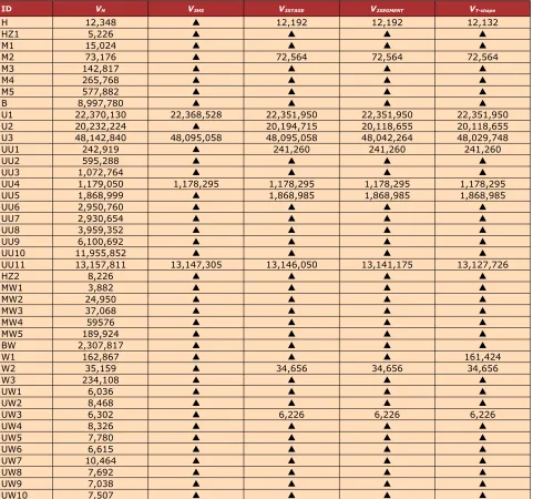
ID VN V3HS V3STAGE V2SEGMENT VT-shape

H 12,348 ▲ 12,192 12,192 12,132

HZ1 5,226 ▲ ▲ ▲ ▲

M1 15,024 ▲ ▲ ▲ ▲

M2 73,176 ▲ 72,564 72,564 72,564

M3 142,817 ▲ ▲ ▲ ▲

M4 265,768 ▲ ▲ ▲ ▲

M5 577,882 ▲ ▲ ▲ ▲

B 8,997,780 ▲ ▲ ▲ ▲

U1 22,370,130 22,368,528 22,351,950 22,351,950 22,351,950

U2 20,232,224 ▲ 20,194,715 20,118,655 20,118,655

U3 48,142,840 48,095,058 48,095,058 48,042,264 48,029,748

UU1 242,919 ▲ 241,260 241,260 241,260

UU2 595,288 ▲ ▲ ▲ ▲

UU3 1,072,764 ▲ ▲ ▲ ▲

UU4 1,179,050 1,178,295 1,178,295 1,178,295 1,178,295

UU5 1,868,999 ▲ 1,868,985 1,868,985 1,868,985

UU6 2,950,760 ▲ ▲ ▲ ▲

UU7 2,930,654 ▲ ▲ ▲ ▲

UU8 3,959,352 ▲ ▲ ▲ ▲

UU9 6,100,692 ▲ ▲ ▲ ▲

UU10 11,955,852 ▲ ▲ ▲ ▲

UU11 13,157,811 13,147,305 13,146,050 13,141,175 13,127,726

HZ2 8,226 ▲ ▲ ▲ ▲

MW1 3,882 ▲ ▲ ▲ ▲

MW2 24,950 ▲ ▲ ▲ ▲

MW3 37,068 ▲ ▲ ▲ ▲

MW4 59576 ▲ ▲ ▲ ▲

MW5 189,924 ▲ ▲ ▲ ▲

BW 2,307,817 ▲ ▲ ▲ ▲

W1 162,867 ▲ ▲ ▲ 161,424

W2 35,159 ▲ 34,656 34,656 34,656

W3 234,108 ▲ ▲ ▲ ▲

UW1 6,036 ▲ ▲ ▲ ▲

UW2 8,468 ▲ ▲ ▲ ▲

UW3 6,302 ▲ 6,226 6,226 6,226

UW4 8,326 ▲ ▲ ▲ ▲

UW5 7,780 ▲ ▲ ▲ ▲

UW6 6,615 ▲ ▲ ▲ ▲

UW7 10,464 ▲ ▲ ▲ ▲

UW8 7,692 ▲ ▲ ▲ ▲

UW9 7,038 ▲ ▲ ▲ ▲

UW10 7,507 ▲ ▲ ▲ ▲

Table 2. The computation results of different layouts

From tables, we can draw conclusions: 1) The optimal results of this paper’s algorithm are equal or very close to the general algorithm; 2) The optimal results of this paper’s algorithm are better than the classic three-stage, two-segment, T-shape.

Layouts 3HS 3STAGE 2SEGMENT T-shape

The optimal number of problems 39 32 32 31

Table 3. The optimal number of different layouts

2SEGMENT and T-shape layout’s optimal results is 32, 32 and 31 respectively. Therefore, the results of this paper algorithm are better than other layouts.

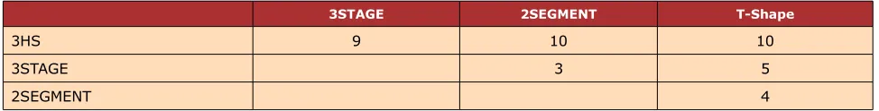
3STAGE 2SEGMENT T-Shape

3HS 9 10 10

3STAGE 3 5

2SEGMENT 4

Table 4. The better number problem of different layouts

Table 4 lists the optimal number of different layouts, and these statistical data come from Table 2. In 43 classical benchmark problems, 1) there are 9 problems that the 3HS layout is better than 3STAGE and 2SEGMENT, and 10 problems for T-shape; 2) there are 3 problems that the 3STAGE layout is better than 2SEGMENT and 5 problems for T-shape; 3) there are 4 problems that the 2SEGMENT layout is better than T-shape. The 3HSA total time it takes for solving 43 problems from table 2 is 93.74s, and each problem’s average time is 2.18s. Therefore, the time is reasonable in practical application.

5. Conclusions

It is very difficult to solve UTDC problem. Although there are exact algorithms, the practical computation results indicate these algorithms only solve small scale problems efficiently. These algorithm’s time it takes for solving large scale problems is unaffordable. Therefore, people usually solve the problem by two types algorithms, first, the algorithms for generating specific layouts, which not only meet the practical production technology, but also solve large scale problems efficiently within reasonable time, for example, the classic three-stage layout, two-segment layout and T-shape layout; second, the results of genetic algorithm is close to general layout algorithm.

References

Alvarez-Valdes, R., Parajon, A., & Tamarit, J.M. (2002). A tabu search algorithm for large-scale guillotine (un)constrained two-dimensional cutting problems. Computers & Operations Research, 29, 925-47. http://dx.doi.org/10.1016/S0305-0548(00)00095-2

Beasley, J.E. (1985). Algorithms for unconstrained two-dimensional guillotine cutting. Journal of the Operational Research Society, 36, 297-306. http://dx.doi.org/10.1057/jors.1985.51

Cui, Y. (2004a). Generating optimal T-shape cutting patterns for rectangular blanks. Journal of Engineering Manufacture, 218, 857-866. http://dx.doi.org/10.1243/0954405041486037

Cui, Y. (2013). A new dynamic programming for three staged cutting patterns. Journal of global optimization, 55, 349-357. http://dx.doi.org/10.1007/s10898-012-9930-3

Cui, Y., Wang, Z., & Li, J. (2005). Exact and heuristic algorithms for staged cutting problems.

Journal of Engineering Manufacture, 219, 201-208. http://dx.doi.org/10.1243/95440505X8136

Fayard, D., & Zissimopoulos, V. (1995). An approximation algorithm for solving unconstrained two-dimensional knapsack problems. European Journal of Operational Research, 84, 618-632. http://dx.doi.org/10.1016/0377-2217(93)E0221-I

Gilmore, P.C., & Gomory, R.E. (1965). Multistage cutting problems of two and more dimensions. Operations Research, 13, 94-119. http://dx.doi.org/10.1287/opre.13.1.94

Han, W., Bennell, J.A., & Zhao, X.Z. (2013). Construction heuristics for two-dimensional irregular shape bin packing with guillotine constraints. European journal of operational research, 230, 495-504. http://dx.doi.org/10.1016/j.ejor.2013.04.048

He, Y.H., & Wu, Y. (2013). Packing non-identical circles within a rectangle with open length.

Journal of global optimization, 56, 1187-1215. http://dx.doi.org/10.1007/s10898-012-9948-6

Hifi, M. (2001). Exact algorithms for large-scale unconstrained two and three staged cutting problems. Computational Optimization and Applications, 18, 63-88.

http://dx.doi.org/10.1023/A:1008743711658

Hifi, M., & Zissimopoulos, V. (1996). A recursive exact algorithm for weighted two-dimensional cutting. European Journal of Operational Research, 91, 553-564. http://dx.doi.org/10.1016/0377-2217(95)00343-6

Ji, J., Lu, Y., & Cha, J. (2012). A deterministic algorithm for optimal two-segment cutting patterns of rectangular blanks. Chinese Journal of Computers, 35(1), 183-191.

http://dx.doi.org/10.3724/SP.J.1016.2012.00183

Jiang, X., Lv, X., & Liu, C. (2008). Optimal Packing of Rectangles with an Adaptive Simulated Annealing Genetic Algorithm. Journal of Computer-Aided Design & Computer Graphics, 11, 1425-1431.

Kellerer, H., Pferschy, U., & Pisinger, D. (2004). Knapsack problems, Berlin ： Springer.

http://dx.doi.org/10.1007/978-3-540-24777-7

Liu, Z., & Liu, J. (2011). Simulated Annealing Algorithm for Solving Circular Packing Problem.

Computer Engineering, 37, 197-199.

Seong, G.G., & Kang, M.K. (2003). A best-first branch and bound algorithm for unconstrained two-dimensional cutting problems. Operations Research Letters, 3 1 , 3 0 1 - 3 0 7 .

http://dx.doi.org/10.1016/S0167-6377(03)00002-6

Thomas, J., & Chaudhari, N.S. (2013). Hybrid approach for 2D strip packing problem using genetic algorithm. Advances in notes in computer science, 7902, 566-574.

Journal of Industrial Engineering and Management, 2014 (www. jiem. org)

Article's contents are provided on a Attribution-Non Commercial 3. 0 Creative commons license. Readers are allowed to copy, distribute and communicate article's contents, provided the author's and Journal of Industrial Engineering and Management's names are included.