Reconstructed Radial Basis Function Networks
Bo-Hyun Kim, Daewon Lee, and Jaewook Lee Department of Industrial and Management Engineering,
Pohang University of Science and Technology, Pohang, Kyungbuk 790-784, Korea
Abstract. Modelling volatility smile is very important in financial prac-tice for pricing and hedging derivatives. In this paper, a novel learning method to approximate a local volatility function from a finite mar-ket data set is proposed. The proposed method trains a RBF network with fewer volatility data and finds an optimized network through op-tion pricing error minimizaop-tion. Numerical experiments are conducted on S&P 500 call option market data to illustrate a local volatility surface estimated by the method.
1
Introduction
Volatility is known as one of the most important market variable in financial practice as well as in financial theory, although it is not directly observable in the market. The celebrated Black-Scholes (BS) model that assumes constant volatility has been widely used to estimate volatility (often calledimplied volatil-ity since it calculates the volatility by inverting the Black-Scholes formula with option price data given by the market) [3, 14]. If the assumption of BS model is reasonable, the implied volatility should be the same for all option market prices.
In reality, however, it has been observed that the implied volatility shows strong dependence on strike price and time to maturity. This dependence, called the volatility smile, cannot be captured in BS model, and results in failure to produce an appropriate volatility for the corresponding option [17, 18].
One practical solution for the volatility smile is the constant implied volatility approach which is to simply use different volatilities for options with different strikes and maturities. In other words, if we had options with the whole range of strikes and maturities, we could simply calculate the implied volatility for each pair of strike and maturity by inverting the BS formula for each option. Although it works well for pricing simple European options, it cannot provide appropriate implied volatilities for pricing more complicated options such as exotic options or American options. Moreover, this approach can produce incorrect hedge factors like Gamma, Vega, Delta, etc. even for simple options [8, 12].
During the last decade, a number of researches based on different type of models have been conducted to model the volatility smile [15, 8, 1, 2]. One of the
J. Wang et al. (Eds.): ISNN 2006, LNCS 3973, pp. 524–530, 2006. c
successful type of model is to use a 1-factor continuous diffusion model. This model, describing volatility as a function of strikes (or stocks) and maturities (called a local volatility function), is turned out to be a complete model by excluding non-traded source of risks and allows for arbitrage pricing and hedging [5]. When the underlying asset follows this model, one important task is then to accurately approximate the local volatility function for accurately pricing exotic options and computing correct hedge factors [4]. Estimating a local volatility function is, however, a nontrivial task since it is generally an ill-posed problem due to insufficient market option price data.
In this paper, we propose a novel learning method to approximate a local volatility function from a finite market data set in pricing and hedging deriva-tives. The proposed method consists of two phases. In the first phase, we train a preparatory radial basis function (RBF) network from an available volatil-ity data to estimate the local volatilvolatil-ity surface and then obtain the estimated volatilities for the whole range of strikes and maturities. In the second phase, we reconstruct an optimized RBF network by controlling the volatility values of a preparatory RBF network to minimize the error between estimated option prices and real market option prices.
The organization of this paper is as follows. In section 2, we propose a learning method to model a volatility smile. Computational simulation applied to the S& P 500 index options are conducted in Section 3. Section 4 concludes the result.
2
The Proposed Method
The 1-factor continuous diffusion model assumes the underlying asset follows the following process with the initial valueSinit:
dSt St
=μ(St, t)dt+σ(St, t)dWt, t∈[0, τ], τ >0 (1) whereτ is a fixed time horizon,Wt is a standard Brownian motion andμ(s, t), σ(s, t) :R+×[0, τ]→Rare deterministic functions sufficiently well behaved to guarantee that (1) has a unique solution [9].σ(s, t) is the local volatility function. When we estimate a local volatility function from a finite data set, we can avoid over-fitting problem by regularizing with some kind of smoothness of the local volatility function. A RBF network is a well-known method that is capable of solving ill-posed problems with regularization [7].
In this section, we propose a method to approximate the local volatility func-tion using RBF networks when the underlying asset follows a 1-factor model (1). The local volatility functionσ(s, t) will be explicitly represented by a recon-structed RBF network.
2.1 Phase I: Initial Local Volatility Function Approximation Using RBF Networks
data set. Each training input has two attributes; strike price and time to ma-turity, (Ktr
j , Tjtr), j = 1, ..., l and training output has its corresponding local volatility value,σj. A RBF network involves searching for a suboptimal solution in a lower-dimensional space that approximates the interpolation solution where the approximated solution ˆσRBF(w) can be expressed as follows:
ˆ
σRBF(w;K, T) = l
j=1
wjφ
(K, T)−(Ktr j , Tjtr) η
(2)
where each φ = φ((K, T),(Ktr
j , Tjtr)) is a radial basis function centered at (Ktr
j , Tjtr) and η is an user pre-specified scale parameter. The training proce-dure of the RBF network is to estimate the weights that connect the hidden and the output layers and these weights will be directly estimated by using the least squares algorithm [7, 6, 11].
To determine the optimal network weights that connect the hidden and the output layers from a training data set,{Ktr
j , Tjtr, σj}lj=1, we fit an initial local
volatility surface by minimizing the following criterion function with a weight decay regularization term
J(w) = l
j=1
σj−ˆσRBF(w;K tr j , T
tr j )
2+λw2. (3)
whereλis a regularization parameter introduced to avoid over-fitting. The net-work weights can then be explicitly given by
w= (Φ+λI)−1σ (4) whereΦ= [φ((Ktr
i , Titr),(Kjtr, Tjtr))]i,j=1,...,landσ= (σ1, ..., σl)T. Substituting Eq. (4) into Eq. (2) makes us to rewrite ˆσRBF(w;K, T) as ˆσRBF(σ;K, T).
Initially, we do not use the training volatility information σ at this stage for the estimated option prices to match the market option prices as closely as possible. Instead, we randomly generate the initial volatility vector,σ(0) ∈ l
in Eq. (4), as nonnegative values. For this reason, we will call the RBF network obtained in the first phase a preparatory RBF network.
2.2 Reconstructing RBF Networks Via Pricing Error Minimization
To obtain a better local volatility function that minimizes the option pricing er-ror, in the second phase, we reconstruct the RBF network by iteratively updating the current volatility vectorσ(0) to a better one.
Letpibe thei-th option market price with (Ki, Ti) as its strike price and matu-rity fori= 1, ..., m. Note that the set{(Ki, Ti)}mi=1 has its corresponding option
pricepi and is a different set from the training input data set{(Kjtr, Tjtr)}lj=1.
an optimal volatility, σ∗ = (σ∗1, ..., σ∗l), to reconstruct a final RBF network by solving the following nonlinear optimization:
min
σ E(σ) =
m
i=1
{pi−Pi[Ki, Ti,σˆRBF(σ;Ki, Ti)]}
2
(5)
+α l
j=1
σjtr−σˆRBF(σ;Kjtr, Tjtr)2
whereσtr
j is a volatility output at a training input (Kjtr, Tjtr) andαis an user-controllable compensation parameter. In this paper, we will call the RBF corre-sponding to this optimal volatilityσ∗as a reconstructed RBF.
To get the optimal solution that minimizes Eq. (5) efficiently, we employ a trust region algorithm described as follows. For a volatility vector σ(n) at iterationn, the quadratic approximation ˆE is defined by the first two terms of the Taylor approximation toE atσ(n);
ˆ
E(s) =E(σ(n)) +g(n)Ts+1 2s
TH(n)s (6)
whereg(n) is the local gradient vector andH(n) is the local Hessian matrix. A trial steps(n) is then computed by minimizing (or approximately minimizing) the trust region subproblem stated by
min s
ˆ
E(s) subject to s2≤Δn (7)
whereΔn>0 is a trust-region parameter. According to the agreement between predicted and actual reduction in the functionE as measured by the ratio
ρn=
E(σ(n))−E(σ(n) +s(n)) ˆ
E(0)−E(ˆ s(n)) , (8)
Δn is adjusted between iterations as follows:
Δn+1=
⎧ ⎨ ⎩
s(n)2/4 ifρn<0.25
2Δn ifρn>0.75 andΔn=s(n)2
Δn otherwise
(9)
The decision to accept the step is then given by
σ(n+ 1) =
σ(n) +s(n) ifρn ≥0
σ(n) otherwise (10)
3
Computational Examples
We use the S&P 500 Index European call option data of October 1995, which is also used in [1, 4]. The market option price data is given in Table 1. Only the options with no more than two years maturity are used for accuracy. The initial index, interest rate, and dividend rate are set as follows:
Sinit = $590, r= 0.06, q= 0.0262
In Phase I, we used the following 16 training volatility input data to train a preparatory RBF network:
(Kjtr, Tjtr) = (K(p), T(q)), j= 4(p−1) +q, p, q= 1, ...,4 K= [0.8000Sinit,0.9320Sinit,1.0640Sinit,1.3940Sinit] T = [0,0.66,1.32,1.98]
In Phase II, we used 70 S&P 500 Index option price data given in Table 1.
Table 1.S&P 500 Index call option price
Maturity Strike(% of spot price)
85% 90% 95% 100% 105% 110% 115% 120% 130% 140% .175 9.13e1 6.28e13.52e1 1.29e1 2.11 1.21e−1 3.73e−2 1.62e−2 1.65e−3 5.14e−4 .425 9.63e1 6.91e14.40e1 2.33e1 8.54 2.26 4.21e−1 1.94e−1 2.77e−2 8.72e−3 .695 1.02e2 7.61e15.26e1 3.26e11.64e1 5.95 1.90 6.04e−1 7.25e−2 2.66e−2 .94 1.07e2 8.22e15.99e1 3.99e12.38e1 1.13e1 4.71 1.78 1.82e−1 4.48e−2 1 1.08e2 8.36e16.16e1 4.16e12.54e1 1.28e1 5.50 2.13 2.27e−1 5.44e−2 1.5 1.17e2 9.44e17.31e1 5.40e13.73e1 2.37e1 1.43e1 7.65 1.85 3.10e−1 2 1.26e2 1.04e18.36e1 6.49e14.82e1 3.42e1 2.36e1 1.47e1 5.65 1.78
The proposed method is compared with a popularly used natural cubic spline method (cf. [4]). The spline approach normally uses the same amount of training data (with a different set of strike prices and maturities) for its knot points as that of option market data to get a reasonable performance. The spline func-tion is then reconstructed from the 70 opfunc-tion market data by minimizing opfunc-tion pricing error with respect to 70 volatility input variables. The criteria for com-parison are pricing error (MSE; mean squared error) and hedging error between predicted volatility and true implied volatility.
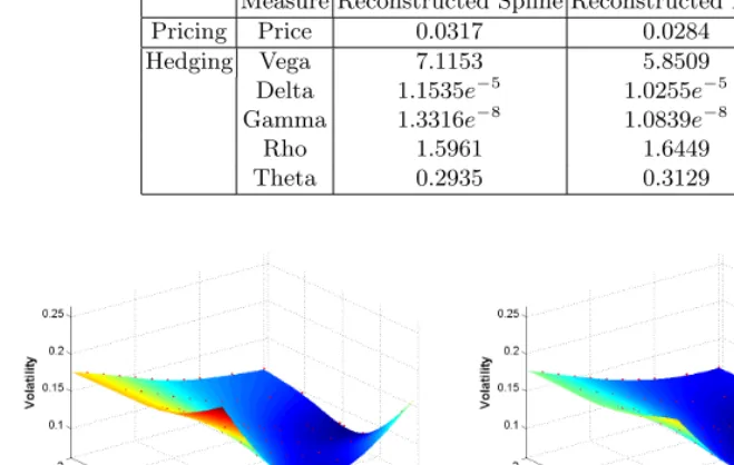
Table 2.Accuracy of Pricing and Hedging
Measure Reconstructed Spline Reconstructed RBF
Pricing Price 0.0317 0.0284
Hedging Vega 7.1153 5.8509
Delta 1.1535e−5 1.0255e−5 Gamma 1.3316e−8 1.0839e−8
Rho 1.5961 1.6449
Theta 0.2935 0.3129
(a) (b)
Fig. 1.Estimated volatility surfaces. (a) spline approach and (b) proposed method.
4
Conclusion
In this paper, we’ve proposed a novel learning method to approximate the local volatility function. The proposed method first trains a preparatory RBF net-work with a training volatility data set to estimate volatility surface and then reconstructs an optimized RBF network by minimizing the errors between es-timated prices and real market prices. A simulation has been conducted with a S&P500 option data example. The experimental results demonstrated a per-formance improvement of the proposed method compared to other approach in terms of pricing and hedging error.
Acknowledgement.This work was supported by the Korea Research Founda-tion under grant number KRF-2004-041-D00785.
References
1. Andersen, L.B.G., Brotherton-Ratcliffe, R.: The Equity Option Volatility Smile: An Implicit Finite Difference Approach. Journal of Computational Finance 1(2) (1997)
3. Black, F., Scholes, M.: The Pricing of Options and Corporate Liabilities. Journal of Political Economy 81 (1973) 637-659
4. Coleman, T.F., Li, Y., Verma, A.: Reconstructing the Unknown Local Volatility Function. The Journal of Computational Finance 2(3) (1999)
5. Dupire, B.: Pricing with a Smile. Risk 7 (1994) 18-20
6. Han, G.S., Lee, D., Lee J. : Estimating The Yield Curve Using Calibrated Radial Basis Function Networks. Lecture Notes in Computer Science 3497 (2005) 885-890 7. Haykin, S.: Neural Networks: a Comprehensive Foundation. Prentice-Hall New
York (1999)
8. Hull, J., White, A.: The Pricing of Options on Assets with Stochastic Volailities. Journal of Finance 3 (1987) 281-300
9. Lamberton, D., Lapeyre, B.: Introduction to Stochastic Calculus Applied to Fi-nance. Chapman & Hall (1996)
10. Lee, J.: Attractor-Based Trust-Region Algorithm for Efficient Training of Multi-layer Perceptrons. Electronics Letters 39 (2003) 71-72
11. Lee, D., Lee, J.: A Novel Three-Phase Algorithm for RBF Neural Network Center Selection. Lecture Notes in Computer Science 3173 (2005) 350-355
12. Lee, H.S., Lee, J., Yoon, Y.G., Kim, S.: Coherent Risk Meausure Using Feedfoward Neural Networks. Lecture Notes in Computer Science 3497 (2005) 904-909 13. Lee, J., Chiang, H.D.: A Dynamical Trajectory-Based Methodology for
Systemat-ically Computing Multiple Optimal Solutions of General Nonlinear Programming Problems. IEEE Trans. on Automatic Control 49(6) (2004) 888 - 899
14. Merton, R.: The Theory of Rational Option Pricing. Bell Journal of Economics and Managemenet Science 4 (1973) 141-183
15. Merton, R.: Option Pricing when Underlying Stock Returns Are Discontinuous. Journal of Financial Economics 3 (1976) 124-144