ISSN 2324-805X E-ISSN 2324-8068 Published by Redfame Publishing URL: http://jets.redfame.com
Actuarial Implications from Pre-kindergarten Education
John Beekman1, David Ober2
1Department of Mathematical Sciences, Ball State University, Muncie, Indiana, USA
2Department of Physics and Astronomy, Ball State University, Muncie, Indiana, USA
Correspondence: David Ober, Department of Physics and Astronomy, Ball State University, Muncie, IN, 47306, USA.
Received: September 12, 2016 Accepted: September 29, 2016 Online Published: October 12, 2016
doi:10.11114/jets.v4i11.1871 URL: http://dx.doi.org/10.11114/jets.v4i11.1871
Abstract
Great progress has been made in providing pre-kindergarten (pre-K) public education throughout the United States. The percentages of 3- and 4-year-olds enrolled nationally have grown from 3% to 5% and 14% to 29%, respectively, between 2002 and 2015. By 2015, 42 states and the District of Columbia were in varying stages of offering pre-K programs (0.9% to 74.2% for totals of 3- and 4-year-olds); eight states were in stages of implementation. We will provide approximate answers to four questions. The first two are how does pre-K education affect female and male life expectancies? The other two are how does pre-K education affect expected years of life dependency in health and in lifetime earnings? The methodology used to help answer these questions consisted of using actuarial/demographic tables over the years 1990 to 2040. It will be shown that upper limits to estimated increases in male and female life expectancy that can be attributed to pre-K education are 2.47 and 1.67 years, respectively. Moderate estimates to the decreases in expected years of health dependency for 65-year old males and females that benefit from pre-K education are 1.47 and 4.71 years, respectively. We will document that people with pre-K education will have higher high school graduation rates, lower crime rates, higher employment rates, and higher wages than those without pre-K education; these four improved rates will lead to improved life expectancies and diminished years of health dependency. These results have actuarial implications for life insurance, long-term health insurance, and pension premium calculations.
Keywords: life expectancies, active life expectancies, years of health dependency, pre-K education 1. Introduction
In this study we will utilize correlations involving three areas of research in order to establish that pre-kindergarten (pre-K) education affects male and female life expectancy; life expectancies and active life expectancies determine years of health dependency. Linking correlations from the three research areas together one is able to establish that pre-K education has actuarial implications.
The three areas of research that will be cited in this study are as follows: first, birth through age five (B5) child development; secondly, the correlations between education and current/lifetime income; and thirdly, the rapidly developing research base that is forming between health, education, and life expectancy. First we will describe the rapid interest, development, and benefits of pre-K education by states. This will be followed by the development of the research questions that will guide the study.
Throughout the United States, there has been considerable emphasis on providing pre-K education for more infants and toddlers. Among many papers on this subject, we would cite papers by Rowe et al. (2012) and Center for Public Education (2008). The first paper documents that a toddler’s vocabulary at 54 months can be predicted by the child’s vocabulary at 30 months, socioeconomic status, and parent-child interactions during the first months of life.
or reduced lunch, and those not participating in the subsidy program. Hispanic children exhibited an eleven-month gain in letter-word recognition and six-month gain in applied problem solving compared to the corresponding gains for white children (nine months and three months, respectively). Recent studies in Michigan, New Jersey, Oklahoma, South Carolina, and West Virginia found children in state pre-K posted vocabulary scores that were 31 percent higher and math gains that were 44 percent higher than those of non-participants. Participants had an 85 percent increase in print awareness, which suggests these outcomes strongly predict later reading success.
1.1 Long-term Benefits of pre-K Education
Long-term pre-K research has focused on whether program effects fade out over time or produce lasting benefits for the participants. Three major longitudinal studies which began in the 1960s and 1970s show demonstrably positive effects of quality pre-K on the future lives of young children. One study followed former program participants and a control group through age 40. In one study, low-income black children randomly selected to receive the comprehensive pre-school program showed impressive long-term results regarding educational progress, delinquency, and earnings. Seventy-seven percent of these students graduated from high school, compared with 60 percent of the control group. In adulthood pre-K participants were less likely to be arrested for violent crimes, more likely to be employed, and more likely to earn higher wages than those in the comparison group.
One of the studies compares students with pre-K versus students without pre-K in five categories; for simplicity we refer to these comparison groups as group 1 and group 2, respectively. Sixty-seven percent of group 1 had IQs over 90 at age 5, versus 28 percent of group 2. Forty-nine percent of group 1 achieved basic or better test results at age 14, versus 15 percent of group 2. Sixty-five percent of group 1 graduated from high school, versus 45 percent of group 2. Twenty-seven percent of group 1 owned their home at age 27, versus five percent of group 2. Sixty percent of group 1 earned over $20,000 at age 40 versus 40 percent of group 2.
High quality pre-K programs provide substantial cost savings to federal, state, and local governments. Numerous studies have shown a reduced use of special education services and lower grade retention among pre-K participants. Economic analyses have quantified these benefits and other societal outcomes (i.e., less delinquency, decreased dependence on public assistance, and increased employment and earnings). These benefits and outcomes are summarized in Table 1.
Table 1. Benefits per Participant
Study 1 Study 2 Study 3 At Age 27 At Age 22 At Age 21 Benefits per $1 Invested
to pre-K Participants and the Public $8.74 $3.78 $10.15 Source: Committee for Economic Development 2006
1.2 Research Questions
We have examined these topics as they relate to poverty and the associated delays in child development and achievement in Grissmer, Beekman, Ober (2014), Beekman and Ober (2015), and Ober and Beekman (2016). These papers analyze pre-K achievement delays that occur from socioeconomic status, the subsequent poverty impacts on children in a state's primary and secondary educational performance, and post-secondary education career selection.
In preparing this paper, we are seeking approximate answers to the following four questions:
1) How does pre-K education affect female life expectancy?
2) How does pre-K education affect male life expectancy?
3) How does pre-K education affect expected years of life dependency in health?
4) How does pre-K education affect lifetime earnings?
The answers to these questions all have actuarial implications. We will provide approximate answers, recognizing that each question pertains to a very large subject.
2. Analyses and Results
The methodology used in this study consisted of first using actuarial/demographic tables over the years 1990 to 2040 to determine gains in female and male life expectancies over segments of those years. Secondly, actuarial/demographic tables of active life expectancies for females and males were obtained for the same period. Active life expectancies relate to years of independence in the activities of bathing, dressing, transfer, and eating.
2040 provides gains between one year and a later year for life expectancy, and active life expectancy, and declines in health dependency.
Projected gains in life expectancy and active life expectancy, and declines in health dependency have actuarial implications for life insurance, long-term health insurance, and pension premium calculations. Such gains are affected by low-, intermediate-, or high-cost assumptions for mortality.
2.1 Initial Approximate Answers to Questions 1 and 2
We will first use Social Security Period Life Tables for 1990, 2000, and 2010, and male life expectancies and female life expectancies for those years to provide approximate answers to questions one and two. After examining differences in male life expectancies and female life expectancies for the years 1990 to 2000, and 2000 to 2010, we will calculate 25%, 50%, and 75% of such differences. They are possible percentage gains in life expectancies due to pre-K education. It seems very difficult to justify some percentage as being the best estimate. Moreover, probably no researchers could develop completely precise answers to the four questions.
The Office of the Chief Actuary, Social Security Administration, Baltimore, Maryland, developed the Period Life Tables. See Wade (1989) and Bell, Wade, and Goss (1992). “Life Expectancy, Average Life Expectancy, and the Interface of Health and Education” relates to our use of the percentage gains of 25%, 50%, and 75% as possible gains in life expectancies, active life expectancies, and a lower number of years of life dependency in health. The percentage gains were applied to the 1990, 2000, and 2010 averages to produce Table 2.
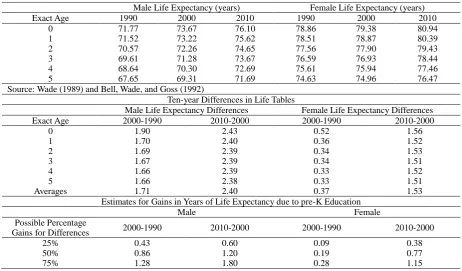
Table 2. Social Security Period Life Tables for 1990, 2000, and 2010
Male Life Expectancy (years) Female Life Expectancy (years)
Exact Age 1990 2000 2010 1990 2000 2010
0 71.77 73.67 76.10 78.86 79.38 80.94
1 71.52 73.22 75.62 78.51 78.87 80.39
2 70.57 72.26 74.65 77.56 77.90 79.43
3 69.61 71.28 73.67 76.59 76.93 78.44
4 68.64 70.30 72.69 75.61 75.94 77.46
5 67.65 69.31 71.69 74.63 74.96 76.47
Source: Wade (1989) and Bell, Wade, and Goss (1992)
Ten-year Differences in Life Tables
Male Life Expectancy Differences Female Life Expectancy Differences
Exact Age 2000-1990 2010-2000 2000-1990 2010-2000
0 1.90 2.43 0.52 1.56
1 1.70 2.40 0.36 1.52
2 1.69 2.39 0.34 1.53
3 1.67 2.39 0.34 1.51
4 1.66 2.39 0.33 1.52
5 1.66 2.38 0.33 1.51
Averages 1.71 2.40 0.37 1.53
Estimates for Gains in Years of Life Expectancy due to pre-K Education
Male Female
Possible Percentage
Gains for Differences 2000-1990 2010-2000 2000-1990 2010-2000
25% 0.43 0.60 0.09 0.38
50% 0.86 1.20 0.19 0.77
75% 1.28 1.80 0.28 1.15
Note: The percentage gains were applied to the averages to produce these tables.
2.2 Secondary Approximations to Questions 1 and 2
Table 3. Social Security Life Tables for 2000, 2020, and 2040
Year
Life Expectancy (years) e0x at Age 0
Male Female
2000 74.03 79.39
2020 76.50 80.80
2040 78.46 82.47
Source: Bell and Miller (2005)
Difference
Twenty-year Differences in Life Table Projections, Ages 0
Years Male Female
2000-2020 2.47 1.41
2020-2040 1.96 1.67
Gains in Years of Life Expectancy
Male Female
Possible Percentage Gains for Differences 2000-2020 2020-2040 2000-2020 2020-2040
25% 0.62 0.49 0.35 0.42
50% 1.24 0.98 0.70 0.84
75% 1.85 1.47 1.06 1.25
2.3 Active Life Expectations
The projected gains in life expectancies at age 0 have actuarial implications for life insurance and pension premium calculations. For this longer and more current time span of 2000 to 2040, we wish to expand our analysis to include active life expectancies. The concept of active life expectancy was originated in the paper Katz et al. (1983). Such expectancy provides a measure of the expected number of years of independence in certain Activities of Daily Living (ADL). Katz et al. (1983) used bathing, dressing, transfer, and eating as ADL. In 1974 Katz et al. (1983) interviewed 1625 noninstitutionalized elderly people in Massachusetts and constructed their ADL scores. In early 1976, data were gathered from 89% of the 1625 original respondents. From the 1225 people who in 1974 were independent in ADL, proportions were calculated of those who lost independence in ADL, or died during the study period. Tables of active life expectancy for males and females were developed.
The paper by Beekman and Frye (1991) provided tables of active life expectancy at age 65, (a0e)65, for the years 1990
and 1995, and for each decade between 2000 and 2080 under three sets of assumptions for regular life expectancies 0e65.
Those expectancies came from Table 10 of Wade (1989). Alternative I assumes low life expectancies, Alternative II assumes intermediate values for life expectancies, and Alternative III assumes high life expectancies.
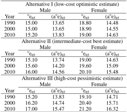
We use excerpts from Table 7 of Beekman and Frye (1991) to produce projections of life and active life expectancies for the years 1990, 2000, and 2010. In 1991, years 2000 and 2010 were future years. We will show the projections under Alternatives I, II, and III for life expectancy values. The expression (oex - (aoe)x) represents the expected years of
dependency for a person aged x. Such values will be dependent on what assumption is made about future life expectancies. To illustrate these ideas, Table 4 permits one to calculate expected years of dependency for the years 1990, 2000, and 2010 for persons aged 65 under Alternatives I, II, and III for life expectancy values, the low-cost optimistic estimate, the intermediate-cost best estimate, and the high-cost pessimistic estimate, respectively (Board of Trustees 2015).
Table 4. Projections of Life and Active Life Expectancies
Alternative I (low-cost optimistic estimate)
Male Female
Year oe65 (a o
e)65 o
e65 (a
o
e)65
1990 15.00 13.65 18.80 14.48 2000 15.00 13.65 18.90 14.55 2010 15.20 13.83 19.00 14.63 Alternative II (intermediate-cost best estimate)
Male Female
Year oe
65 (aoe)65 oe65 (aoe)65
1990 15.10 13.74 19.00 14.63 2000 15.60 14.20 19.60 15.09 2010 16.00 14.56 20.10 15.48 Alternative III (high-cost pessimistic estimate)
Male Female
Year oe65 (aoe)65 oe65 (aoe)65
2.4 Answers to Question 3
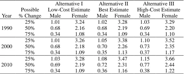
In future years, more and more people will benefit from pre-K education, thus reducing the health expenses caused by years of dependency. To illustrate this, we will consider possible gains of 25%, 50%, and 75%. We will use Table 5 to produce Table 6, which relates to Question 3, how does pre-K education affect expected years of life dependency in health?
Table 5. Expected Years of Dependency for a person aged 65
Alternative I Low-Cost Estimate
Alternative II Best Estimate
Alternative III High-Cost Estimate Year Male Female Male Female Male Female 1990 1.35 4.32 1.36 4.37 1.37 4.39 2000 1.35 4.35 1.40 4.51 1.46 4.69 2010 1.37 4.37 1.44 4.62 1.53 4.88
There are observations that can be made from Tables 4, 5, and 6. We see from Table 4 that oe65 increases from
Alternatives I to II, from II to III for both male and female. Also, aoe65 increases from Alternatives I to II to III for both male and female. From Table 5 oe65 - (aoe)65 also increases from Alternatives I to II, from II to III for both male and
female. Thus, although both the life and active life expectancies are increasing as the projected years grow, so do the expected years of dependency. Fortunately, those last gains are very small.
Table 6. Expected Years of Dependency for a 65-yr Old Who Benefitted from Pre-Kindergarten Education
Possible
Alternative I Low-Cost Estimate
Alternative II Best Estimate
Alternative III High-Cost Estimate Year % Change Male Female Male Female Male Female
1990
25% 1.01 3.24 1.02 3.28 1.03 3.29
50% 0.68 2.16 0.68 2.19 0.69 2.20
75% 0.34 1.08 0.34 1.09 0.34 1.10
2000
25% 1.01 3.26 1.05 3.38 1.10 3.52
50% 0.68 2.18 0.70 2.26 0.73 2.35
75% 0.34 1.09 0.35 1.13 0.37 1.17
2010
25% 1.03 3.28 1.08 3.47 1.15 3.66
50% 0.69 2.19 0.72 2.31 0.77 2.44
75% 0.34 1.09 0.36 1.16 0.38 1.22
From Table 6, [(1 - f) (oe65 - (a o
e)65)] values decrease as f moves from f = 0.25 to f = 0.50 to f = 0.75. That is logical
because as the benefit from pre-K education increases, the years of dependence decrease.
2.5 Projections of Active Life Expectancies
We now use excerpts from Table 7 of Beekman and Frye (1991) to produce projections of life and active life expectancies for the years 2000, 2020, and 2040. We will show the projections under the Alternatives I, II, and III for life and active life expectancies. Recent 20-year spans in life expectancies come from Bell and Miller (2005).
We will use portions of Table 7 of Active Life Expectancies (Beekman and Frye 1991) to obtain projections of active life expectancies for ages 65 through 99. The Alternative II (intermediate best estimate) values from Table 7 for age 65 for years 2010, 2020, 2030, and 2040 were used. Such values assume intermediate values for life expectancies. The Active Life Expectancies in Table 7 of this paper, all for age 65, were created by assuming a simple arithmetic growth from the years 1990, 1995, 2000,..., 2080.
A companion table to Table 5 is shown in Table 8.
From the values for life expectancy, and active life expectancy at age 65, we calculated the ratios of active life expectancy to life expectancy for males and females. The values were 0.8475 and 0.7854. We then created comparable ratios at ages 75, 85, 95, and 99.The male ratios were 0.75, 0.55, 0.25, and 0.10, and the female ratios were 0.68, 0.48, 0.28, and 0.10. With these rounded ratios, we created projections of active life expectancies, and projections of expected years of health dependency for single ages 66, 67, ..., 99, for males and females.
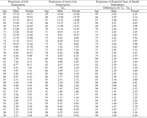
Presented in Figure 1 and Table A of Appendix A are the six projections of expected years of life expectancy, active life expectancy, and expected years of health dependency for males and females from age 65 through 99.
The projected gains over the years 2000 to 2040 in life and active life expectancies, and expected years of dependency at age 65for males and females, for alternatives I, II, and III for life expectancy values have actuarial implications for health insurance premium calculations.
A comparison table to Table 6 is shown in Table 9.
Tables 7, 8, and 9 are larger than the comparable numbers from Tables 4, 5, and 6. However, the patterns for oe65, (a o
e)65, o
e65 - (a o
e)65, and [(1 - f) ( o
e65 - (a o
e)65)] for f = 0.25, 0.50, and 0.75, are the same.
Table 7. Projections of Life and Active Life Expectancies
Alternative I (low-cost optimistic estimate)
Male Female
Year oe65 (aoe)65 oe65 (aoe)65
2000 15.0 13.65 18.9 14.55
2020 15.3 13.92 19.2 14.78
2040 15.7 14.29 19.6 15.09
Alternative II (intermediate-cost best estimate)
Male Female
Year oe65 (aoe)65 oe65 (aoe)65
2000 15.6 14.20 19.6 15.09
2020 16.4 14.92 20.5 15.79
2040 17.1 15.66 21.4 16.48
Alternative III (high-cost pessimistic estimate)
Male Female
Year oe65 (a o
e)65 o
e65 (a
o
e)65
2000 16.2 14.74 20.4 15.71
2020 17.8 16.20 22.0 16.94
2040 19.3 17.56 23.7 18.25
Source: Beekman and Frye 1991
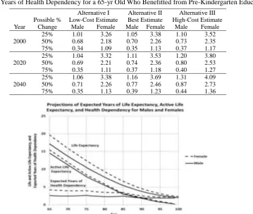
Table 8. Expected Years of Dependency for a person aged 65
Alternative I Low-Cost Estimate
Alternative II Best Estimate
Alternative III High-Cost Estimate Year Male Female Male Female Male Female 2000 1.35 4.35 1.40 4.51 1.46 4.69 2020 1.38 4.42 1.48 4.71 1.60 5.06 2040 1.41 4.51 1.54 4.92 1.74 5.45
Table 9. Expected Years of Health Dependency for a 65-yr Old Who Benefitted from Pre-Kindergarten Education
Possible %
Alternative I Low-Cost Estimate
Alternative II Best Estimate
Alternative III High-Cost Estimate Year Change Male Female Male Female Male Female
2000
25% 1.01 3.26 1.05 3.38 1.10 3.52
50% 0.68 2.18 0.70 2.26 0.73 2.35
75% 0.34 1.09 0.35 1.13 0.37 1.17
2020
25% 1.04 3.32 1.11 3.53 1.20 3.80
50% 0.69 2.21 0.74 2.36 0.80 2.53
75% 0.35 1.11 0.37 1.18 0.40 1.27
2040
25% 1.06 3.38 1.16 3.69 1.31 4.09
50% 0.71 2.26 0.77 2.46 0.87 2.73
75% 0.35 1.13 0.39 1.23 0.44 1.36
2.6 An Answer to Question 4
Question 4 asks, "How does pre-K education affect lifetime earnings?" To answer this question the United States Bureau of Labor Statistics periodically provides information that compares the unemployment rates and wages of workers with differing levels of educational training. Presented in Table 10 are comparisons for 2014. The unemployment rates and median weekly earnings in 2014 for those with less than a college bachelors-degree range from 9.0% to 4.5% and $488 to $792, respectively, for those with less than a high school diploma, a high school diploma, an associate degree, and some college training (no degree). However, those with a four-year college bachelor's degree or more have 2014 unemployment rates and median weekly earnings ranges of 3.5% to 1.9% and $1101 to $1591, respectively, for bachelors, masters, professional, and doctoral degrees. (These data are for persons age 25 and over, and they are for full-time and salaried workers.)
Table 10. Earnings and unemployment rates by educational attainment
Education Attained 2014 Unemployment Rate (Percent)
Median Weekly Earnings in 2014
Doctoral Degree 2.1 $1,591
Professional Degree 1.9 $1,639
Master's Degree 2.8 $1,326
Bachelor's Degree 3.5 $1,101
All Workers 5.0 $839
Associate's Degree 4.5 $792
Some College, no Degree 6.0 $741
High School Diploma 6.0 $668
Less than a High School Diploma 9.0 $488
Note: Data are for persons age 25 and over. Earnings are for full-time wage and salary workers. Source: Current Population Survey, U.S. Department of Labor, U.S. Bureau of Labor Statistics http://www.bls.gov/emp/ep_table_001.
3. Discussion
The final key to linking pre-K education and actuarial implications is to document the correlations between improvements in health with education and family income. The following studies by medical researchers have examined life expectancies for specific diseases by education levels, gender, and ethnicity.
3.1 Life Expectancy, Average Life Expectancy, and the Interface of Health and Education
Outstanding talks given at 2014 Institute of Medicine meetings (Alper, J., Thompson, D., & Baciu, A. (Eds.), 2015) by Dr. Stephen Woolf (2014) and Dr. Robert Kaplan (2014) discussed life expectancies, disability-free years, and their connections with education. Also at these meetings Dr. Peter Orszag (2014) provided excellent insight into the connections between education and health, and how they will both be better served in the long term when improvements are accomplished together.
Kaplan cited the work of Zimmerman and Woolf (2014) to review how education has long been identified as a key correlate in explaining health disparities and predicting health outcomes. The research by Basch (2011) was used to illustrate how health influences student performance and leads to achievement gaps between ethnic groups and students of differing socioeconomic status. Evidence from the study by Olshansky et al. (2012) provided evidence of gaps in life expectancy by ethnicity and level of education; of particular interest and somewhat surprising were the results in a comparison of life expectancy at birth, by years of education at age 25 for white females for 1990, 2000, and 2008, where there was a decrease for females with less than 12 years of education while steady increases were exhibited by years of education as well as for the three years studied. Kaplan also reported that adverse childhood events affect life expectancy in adults which can be correlated with diabetes, heart disease, and obesity (Montez and Hayward, 2014).
Woolf (2014) addressed one of the major topics of the conference (Alper et al., 2015) by citing the research connecting the improvement of health with levels of attainment of education. For example, he used the work of Ross et al. (2012) to state how life expectancy of U.S adults by age 25 and without high school diplomas is projected to live nine years less than college graduates. The results of Olshansky et al. (2012) were used to demonstrate that no changes had occurred in life expectancies for both males and females who had high school diplomas, as they had the same life expectancies in 2008 that they had in 1972 and 1964, respectively.
4. Conclusions
This study has linked the fields of B5 child development, education and current/lifetime income, and medical health research in order to provide demographics that link education, gender, and ethnicity with life expectancy. A methodology was then used to determine gains in female and male life expectancies and active life expectancies using Social Security Period Life tables. From these tables male and female health dependency values were obtained making it possible to provide upper bounds to gains between one year and a later year for life expectancy, active life expectancy, and health dependency.
This paper has shown possible projected gains in life expectancies, active life expectancies, and a lower number of years of life dependency in health due to pre-K education. We used 25%, 50%, and 75% as possible gains in the above three quantities over time intervals due to pre-K education. Such gains in the three quantities of interest are shown in Tables 2, 3, 6, and 9.
Specifically, research Questions 1 and 2 (how pre-K education affects female and male life expectancy, respectively) are partially answered in Table 2. The average age 0 to 5 increase in life expectancy for males was 1.71 and 2.40 years, and the average increase for females was 0.37 and 1.53 years for the 2000-1990 and 2010-2000 differences, respectively. These differences were then used to compute corresponding 25%, 50%, and 75% amounts that one could possibly attribute to pre-K education.
Table 3 also provides partial answers to research Questions 1 and 2. The age 0 increase for life expectancy of males was 2.47 and 1.96 years, and the increase for females was 1.41 and 1.67 years for the 2020-2000 and 2040-2020 differences, respectively. Again, differences were then computed for 25%, 50%, and 75% of those amounts that one could possibly attribute to pre-K education.
Research Question 3 (how pre-K education affects expected years of life dependency in health) is answered with Table 6 by first computing the 1990, 2000, and 2010 life expectancies and active life expectancies at age 65 (Table 4) for pessimistic, moderate, and optimistic alternatives. Differences between the years 2000-1990 and 2010-2000 life expectancy/active life expectancy differences then yielded expected years of life dependency at age 65. (Table 5) for the three alternatives; the Alternative II (moderate) best estimates for the age 65 males and females averaged 1.40 and 4.50 years, respectively. Table 6 was then obtained taking 25%, 50%, and 75% of Table 5 amounts (and their associated alternatives) to obtain the possible years of life with health dependency and attributed to pre-K education.
If one conducts the analyses just described for research Question 3, but uses age 65 life expectancy and active life expectancy data for the years 2000, 2020, and 2040 (Table 7), the Alternative II (moderate) best estimates for the age 65 males and females averaged 1.47 and 4.71 years, respectively, for the gain in expected years of life dependency (Table 8). As described for Table 6, Table 9 was obtained by taking 25%, 50%, and 75% of Table 8 amounts (and their associated alternatives) to obtain the possible years of life with additional health dependency and attributed to pre-K education.
Research Question 4 (how pre-K education affects lifetime earnings) is answered in Table 10. Table 10 relates to the higher wage earnings and lower unemployment partially due to the initial thrust of learning due to pre-K education. The projected gains in the three quantities of interest – life expectancy, active life expectancy, and expected years of health dependency - have actuarial implications for life insurance, pension premiums, and reserve calculations.
It has also been documented that higher high school graduation rates, lower crime rates, higher employment rates, and higher wages are associated with people with pre-K education when compared to those without pre-K education. Consequently, these four improved rates lead to predictions of improved life expectancies, and diminished years of health dependency which will have actuarial implications on life insurance rates, long-term health insurance rates, and pension calculations.
Acknowledgements
The authors are grateful for helpful comments and additional references provided by Karen B. Eden, Ph.D., Department of Medical Informatics and Clinical Epidemiology, Oregon Health and Sciences University, Portland, Oregon, and Elias S. Shiu, Ph.D., Department of Statistics and Actuarial Science, University of Iowa, Iowa City, Iowa.
References
Alper, J., Thompson, D., & Baciu, A. (Eds.). (2015). Exploring Opportunities for Collaboration Between Health and Education to Improve Population Health: Workshop Summary. R. Kaplan, 2014. Chapter: 1 Introduction and overview, and S. Woolf, 2014. Chapter: 2 Why Educational Attainment Is Crucial to Improving Population Health. National Academies Press.
coordinated school health programs must be a fundamental mission of schools to help close the achievement gap.
Journal of School Health, 81(10), 650-662. http://dx.doi.org/10.1111/j.1746-1561.2011.00640.x
Beekman, J. A., & Frye, W. B. (1991). Projections of Active Life Expectancies. Actuarial Research Clearing House, 2, 73-87. Retrieved from:
https://www.soa.org/Library/Research/Actuarial-Research-Clearing-House/1990-99/1991/Arch-2/arch91v28.aspx
Beekman, J. A., & Ober, D. (2015). Gender Gap Trends on Mathematics Exams Position Girls and Young Women for STEM Careers. School Science and Mathematics, 115(1), 35-50. http://dx.doi.org/10.1111/ssm.12098
Bell, F. C., & Miller, M. L. (2005). Actuarial Study No. 120. Baltimore, MD: U.S. Department of Health and Human Services; Life Tables for the United States Social Security Area 1900-2100. Retrieved from: https://www.ssa.gov/oact/NOTES/pdf_studies/study120.pdf
Bell, F., Wade, A., & Goss, S., (1992). Actuarial Study No. 107. Baltimore, MD: U.S. Department of Health and Human Services; Life Tables for the United States Social Security Area 1900–2080. Retrieved from:
https://www.ssa.gov/oact/NOTES/pdf_studies/study107.pdf
Board of Trustees 2015 OASDI Report, The 2015 Annual Report of the Board of Trustees of the Federal Old-Age and Survivors Insurance and Federal Disability Insurance Trust, U.S. Government Publishing Office, 95-586 Washington, DC. Retrieved from: "https://www.ssa.gov/oact/tr/2015/tr2015.pdf
Current Population Survey (2015). U.S. Department of Labor, U.S. Bureau of Labor Statistics. Retrieved August 6, 2015: http://www.bls.gov/emp/ep_table_001.htm
Grissmer, D. W., Beekman, J. A., & Ober, D. (2014). Focusing on short-term achievement gains fails to produce long-term gains. Education Policy Analysis Archives, 22, 5. Retrieved from:
http://epaa.asu.edu/ojs/article/view/1218
Kaplan, R. (2014, June 10). Report on the June 4 NIH Meeting on the Evidence for Education Improving Health [Video file]. Retrieved from: http://iom.nationalacademies.org/Activities/PublicHealth/PopulationHealthImprovement RT/2014-JUN-05/Videos/Welcome/3-Kaplan-Video.aspx
Katz, S., Branch, G., Branson, M., Papsidero, J., Beck, J., & Greer, D. (1983). Active life expectancy. New England Journal of Medicine, 309 (20), 1218-1224. http://dx.doi.org/10.1056/NEJM198311173092005
Montez, J. K., & Hayward, M. D. (2014). Cumulative childhood adversity, educational attainment, and active life expectancy among US adults. Demography, 51(2), 413-435. http://dx.doi.org/10.1007/s13524-013-0261-x
Ober, D., & Beekman, J. A. (2016). Dynamic Models of Learning Predict Infant-Toddler Vocabulary Trajectories,
Journal of Education and Training Studies, 4(4), April 2016. Retrieved from: http://redfame.com/journal/index.php/jets/article/view/1215/1263
Olshansky, S. J., Antonucci, T., Berkman, L., Binstock, R. H., Boersch-Supan, A., Cacioppo, J. T., & Jackson, J. (2012). Differences in life expectancy due to race and educational differences are widening, and many may not catch up.
Health Affairs, 31(8), 1803-1813. http://dx.doi.org/10.1377/hlthaff.2011.0746
Orszag, P. (2014, June 10). 6/5, Keynote presentation II: How our nation’s health care expenditures reduce education funding, and better ways to structure our nation’s investments [Video file]. Retrieved from: http://iom.nationalacademies.org/Activities/PublicHealth/PopulationHealthImprovementRT/2014-JUN-05/Videos/ Keynote%20II/11-Orszag-Video.aspx
Ross, C. E., Masters, R. K., & Hummer, R. A. (2012). Education and the gender gaps in health and mortality.
Demography,49(4), 1157–1183. http://dx.doi.org/10.1007/s13524-012-0130-z
Rowe, M. L., Raudenbush, S. W., & Goldin-Meadow, S. (2012). The pace of vocabulary growth helps predict later vocabulary skill. Child development, 83(2), 508-525. http://dx.doi.org/10.1111/j.1467-8624.2011.01710.x
The Research on Pre-K, prepared by Chrisanne Gayl, Center for Public Education, 2008. Retrieved from: http://www.centerforpubliceducation.org/Main-Menu/Pre-kindergarten/Pre-Kindergarten
Wade, A. (1989). Social Security Area Population Projections, 1989, Actuarial Study No. 105, Office of the Actuary, Social Security Administration, Baltimore, MD. Retrieved from:
https://www.ssa.gov/oact/NOTES/pdf_studies/study105.pdf
Woolf, S. (2013, June 5). Beyond health care [Video file Part of the Northern Virginia Health Foundation Health Summit]. Retrieved from: https://www.youtube.com/watch?v=-yd8dluRHfQ
Health [Video file]. Retrieved from:
http://iom.nationalacademies.org/Activities/PublicHealth/PopulationHealthImprovementRT/2014-JUN-05/Videos/ Welcome/4-Woolf-Video.aspx
Zimmerman, E., & Woolf, S. H. (2014). Understanding the relationship between education and health. Discussion Paper, Institute of Medicine, Washington, DC. Retrieved from:
http://www.commed.vcu.edu/Chronic_Disease/2015/education_healthlink.pdf
Appendix A
Table A. Expected Years of Life Expectancy, Active Life Expectancy, and Health Dependency for Males and Females - Ages 65 - 99
Projections of Life Expectancies
Projections of Active Life Expectancies
Projections of Expected Years of Health Dependency
0
ex 0aex Differences of [ 0ex - 0aex ]
Age Male Female Age Male Female Age Male Female
65 17.18 19.71 65 14.56 15.48 65 2.62 4.23
66 16.45 18.92 66 13.90 14.78 66 2.55 4.14
67 15.73 18.15 67 13.23 14.08 67 2.50 4.07
68 15.04 17.40 68 12.57 13.37 68 2.47 4.03
69 14.35 16.65 69 11.90 12.67 69 2.45 3.98
70 13.68 15.92 70 11.24 11.97 70 2.44 3.95
71 13.02 15.20 71 10.57 11.27 71 2.45 3.93
72 12.39 14.49 72 9.91 10.57 72 2.48 3.92
73 11.76 13.80 73 9.24 9.86 73 2.52 3.94
74 11.15 13.11 74 8.58 9.16 74 2.57 3.95
75 10.55 12.44 75 7.91 8.46 75 2.64 3.98
76 9.96 11.78 76 7.42 7.93 76 2.54 3.85
77 9.38 11.14 77 6.93 7.40 77 2.45 3.74
78 8.83 10.51 78 6.44 6.88 78 2.39 3.63
79 8.29 9.90 79 5.95 6.35 79 2.34 3.55
80 7.76 9.31 80 5.46 5.82 80 2.30 3.49
81 7.26 8.73 81 4.96 5.29 81 2.30 3.44
82 6.77 8.17 82 4.47 4.76 82 2.30 3.41
83 6.31 7.63 83 3.98 4.24 83 2.33 3.39
84 5.87 7.11 84 3.49 3.51 84 2.38 3.60
85 5.45 6.62 85 3.00 3.18 85 2.45 3.44
86 5.07 6.16 86 2.77 2.95 86 2.30 3.21
87 4.71 5.72 87 2.53 2.72 87 2.18 3.00
88 4.38 5.30 88 2.30 2.49 88 2.08 2.81
89 4.06 4.91 89 2.06 2.26 89 2.00 2.65
90 3.78 4.55 90 1.83 2.03 90 1.95 2.52
91 3.51 4.22 91 1.60 1.80 91 1.91 2.42
92 3.26 3.91 92 1.36 1.57 92 1.90 2.34
93 3.04 3.63 93 1.13 1.34 93 1.91 2.29
94 2.84 3.37 94 0.89 1.11 94 1.95 2.26
95 2.65 3.14 95 0.75 0.94 95 1.90 2.20
96 2.49 2.94 96 0.62 0.76 96 1.87 2.18
97 2.35 2.76 97 0.48 0.59 97 1.87 2.17
98 2.23 2.59 98 0.35 0.41 98 1.88 2.18
99 2.11 2.44 99 0.21 0.24 99 1.90 2.20