Issues
ISSN: 2146-4138
available at http: www.econjournals.com
International Journal of Economics and Financial Issues, 2017, 7(2), 397-407.
A New Perspective on the Relationship between Trading
Variables and Volatility in Futures Markets
Óscar Carchano
1*, Julio Lucia
2, Ángel Pardo
31Department of Financial Economics, Faculty of Economics, University of Valencia, Avda de los Naranjos s/n, Valencia 46022, Spain, 2Department of Financial Economics, Faculty of Economics, University of Valencia, Valencia, Spain, 3Department of Financial Economics, Faculty of Economics, University of Valencia, Valencia, Spain. *Email: oscar.carchano@uv.es
ABSTRACT
In this paper, we study the relationship between trading-related variables and volatility in futures markets, from a new unifying perspective, which
is based on the separation of open and closed positions. Volatility in stock index futures markets (Standard & Poor’s 500, DAX 30 and Nikkei 225) is related to the flow of contracts entered into the markets and the flow of contracts that are closed out. In general, the daily changes in the number
of open and closed positions are both positively correlated with volatility. Additionally, there is a stronger positive relationship between the number
of open (respectively, closed) positions and contemporaneous volatility on those days when the opening of new positions (respectively, the closing of old ones) dominates the market. Finally, massive intra-day trading does not seem to alter the average volatility. The change in perspective allows us
to provide a consistent story for the effect of the change in the open interest on the volatility analyzed in the previous literature.
Keywords: Volatility, Open Interest, Trading Volume, Open and Closed Positions JEL Classifications: G12, G15
1. INTRODUCTION
A line of research has extensively studied the link among some measure of price variability and several trading-related variables in futures markets. This research has focused on the influence of readily-available trading variables, such as the volume of trading and the open interest, on volatility. Unfortunately, the available literature has provided divergent results, not only regarding its main theoretical conclusions, but also on the basic facts that substantiate them.
Interestingly, a careful study of the literature that analyses volatility, on one hand, and volume and open interest-related variables, on the other, reveals that there is a great deal of heterogeneity on essential issues such as its theoretical foundations and empirical methodologies, not to mention the diversity of sample periods and underlying assets. Broadly speaking, there are two main competing theories behind the analysis of such relationship: One rests on liquidity-related issues, such as market liquidity and market depth, whereas the other relates to the diversity of
traders who participate in futures markets, i.e., informed versus uninformed traders, or speculators versus hedgers. Additionally, the empirical analyses carried out under both lines of reasoning rest fundamentally to some degree on taking some variable related to the volume and open interest variables as proxies for another, sometimes unobservable, variable of interest, which explains the variety of variables defined from the raw volume and open interest figures that have been used in the empirical analyses. Furthermore, this heterogeneity in theoretical foundations and empirical methodologies alike contributes decisively to the lack of a common set of stylized empirical facts in this literature. This state of affairs is highly unsatisfying, because without clear facts it is not possible to reach sound theoretical conclusions.
closed out in any futures contract, based on the daily volume-of-trading and open-interest figures. In particular, we do demonstrate that the joint consideration of the volume of trading and the change in open interest in the analysis of the linkage between daily volatility and trading activity can be interpreted in terms of the number of open and closed positions.
We then analyze empirically the linkage between the daily volatility and these two variables that form the contracting activity in stock index futures markets. To this aim, we estimate a regression that relates a daily volatility measure of the Garman-Klass type derived by Yang–Zhang (2000) to the daily number of contracts that are entered into the market and the daily number of contracts that are closed out, after accounting for the short-term persistence in volatility, for three of the most important stock index futures markets in the world, i.e., Standard & Poor’s 500 (S&P500), DAX 30 and Nikkei 225.
By concentrating on the contracting activity (i.e., the flow of contracts entered into and closed out), we are able to provide new common stylized empirical facts that contribute to the clarification of the relationship between daily volatility and the activity of traders in stock index futures markets. This change in perspective should be of special interest for those researchers dedicated to the study of the microstructure of derivatives markets, because it focuses on the role of the number of open and closed positions in explaining daily volatility.
The remainder of the paper is organized as follows. We first carefully review the available literature that focuses on the influence of the volume of trading and (some variable related to) the open interest on the volatility of futures markets. Our review reveals that this line of previous research does not share a common set of basic facts, and a unique interpretation either. In order to try to shed light on this conundrum, we later explore, both theoretically and empirically, some simple specific combinations of the volume and open interest figures that allow new direct and clear interpretations in terms of the contracting activity that takes place in any given futures market. Throughout the paper, we relate in detail our analysis to the previous literature with a focus on the facts, in accordance with our main objective, although we also connect the facts to possible alternative interpretations.
2. REVIEW OF LITERATURE
In this section, we review the literature devoted to studying the influence on volatility in futures markets of some variable related to the volume of trading and the open interest. We first concentrate on the empirical facts, then we analyze the alternative interpretations that underlie the variety of empirical methodologies.
2.1. Searching for Some Basic Empirical Facts
On one hand, the relation between diverse measures of price variability and the volume of trading for index futures has been investigated extensively. Several studies document a positive and contemporaneous relation between volume and volatility for several stock index futures at different frequencies of data (for example, Kawaller et al., 1994; and Gannon, 1995 for intraday
data, and ap Gwilym et al., 1999; Pati, 2008; Ragunathan and Peker, 1997; Wang and Yau, 2000; Watanabe, 2001 for daily data, and finally Wang, 2002 for weekly data)1. There is additional evidence that indicates that the lagged volume is related to volatility as well. In this case, a negative relationship between lagged volume of trading and price variability is usually found (ap Gwilym et al., 1999; Wang and Yau, 2000 for analyses of stock indexes and other financial underlying assets)2. However, Jena and Dash (2014) and Susheng and Zhen (2014) report the opposite sign for the Nifty index futures and the CSI 300 index futures, respectively.
On the other hand, another variable that has been related with volatility is the level of the open interest in futures markets. The exploration of any additional empirical content related to the open interest, a trading-related variable that is specific to standardized derivative markets, seems in principle attractive. The empirical relationship between open interest and volatility is, however, controversial. Firstly, Watanabe (2001) and Pati (2008) observe a negative link between open interest and volatility in several stock index futures markets. Secondly, Chen et al. (1995) and Jena and Dash (2014) show a positive link, for S&P 500 futures and for the Nifty index futures, respectively. Finally, a group of papers finds a null or weak connection between volatility and open interest. This is the case, for example, of Martinez and Tse (2008) for both stock index and currency futures contracts3. In addition, some variables based on the change in open interest have also been related to the variability of prices (for example, Garcia et al., 1986).
In summary, this previous empirical research based on different methodologies and sample periods unfortunately has provided divergent results.
2.2. On the Diversity of Interpretations
The multiple ways in which the two basic trading-related variables (namely, volume and open interest) have been related to the variability of prices is explained by the variety of interpretations that are assumed for the trading-related variables, based on diverse competing underlying theories. Broadly speaking, there are two main competing theories behind the analysis of such relationship: One rests on liquidity-related issues and the other on the diversity of traders who participate in futures markets.
Following the first line of reasoning, volume and open interest are simply two broad liquidity-related variables for some researchers:
1 Furthermore, there is evidence that also supports a positive relation in the
case of equities (Epps and Epps, 1976; Schwert, 1989 and Smirlock and Starks, 1985), and commodities (Garcia et al., 1986).
2 It seems that this relationship is general for many underlying financial assets. Fung and Patterson (1999) studied five currency futures markets and found the same negative relation between return volatility and past trading volume. In addition, Foster (1995) studied crude oil futures markets, and he determined that lagged volume can partially explain current price variability.
3 A negative relationship is also detected in agricultural, currency, oil and
The volume is taken to be the simplest and more direct liquidity variable and the open interest is considered as a proxy for market depth in futures markets. In this vein, the price variability has also been related to the lagged volume. Wang and Yau (2000), for instance, believed that a lagged change in trading volume implied a reduction in the contemporaneous volatility, taking volume as a measure of liquidity4.
The second line of reasoning follows the intuition of Bessembinder and Seguin (1993), for whom volume and open interest are related to the trading activity carried out by some specific types of traders: The volume of trading is assumed to be a proxy for the trading activity by informed traders, or speculators, whereas the open interest is considered as a proxy for uninformed traders, or hedgers5.
Additionally, several authors combined some trading-related figures into several volume-to-open interest ratios that allegedly provide a better proxy for a given ultimate factor that may be economically related to volatility. Following the latter line of research, Garcia et al. (1986), for example, created a volume-to-open interest ratio in order to measure the relative importance of the speculative behavior in a given contract. ap Gwilym et al. (2002), instead, supported the use of other closely related variables, such as the absolute value of the change in open interest. Lucia and Pardo (2010) show that, instead of the level value of the open interest or the absolute value of the change in open interest, the use of the change in open interest is more appropriate in order to approach the hedging activity (Lucia and Pardo, 2010 for a critique of this line of research).
Notice that the above-mentioned methodological heterogeneity can be at least partially explained by, first, the absence of a unique underlying theory, and second, by the fact that the empirical analysis of both theories rests to some degree on using some variables related to the readily-available volume and open interest figures as proxies for other (sometimes unobservable) variables of interest.
In order to shed light on this conundrum, in what follows we explore some simple specific combinations of the volume and open interest figures that allow new direct and clear interpretations in terms of the contracting activity that takes place in any given
4 Not surprisingly, there are also competing motivations for the inclusion of
lagged volume in the analysis of the relationships of trading-related variables with volatility. Foster (1995) provided two alternative explanations for his finding of the lagged volume partially explaining current price variability in crude oil futures markets. It could be due to traders conditioning their prices on previous trading volume as a measure of market sentiment, or it could be alternatively explained by a form of mimetic contagion where agents set their prices with reference to the trading patterns of other agents. Fung and Patterson (1999) thought that the negative relation between return volatility and past trading volume that they found in currency futures markets was consistent with the overreaction hypothesis observed in the stock market, which suggests a high volume of trading in the stock together with a sharp price response (Conrad et al., 1994).
5 Chesney et al. (2015) relate trading volume and a measure of daily changes in the open interest to detect abnormal trades in option markets, which are interpreted as an indication of informed trading activities (Poteshman, 2006).
futures market. Furthermore, the empirical analysis of such combined variables allow us to provide new common stylized facts for the three stock index futures analyzed in this paper.
3. TRADING-RELATED VARIABLES
In this paper, we relate some trading-related variables to a measure of price variability in futures markets. We begin with an explanation of how the trading variables traditionally related to volatility can be expressed in terms of the number of open and closed positions, which are used as the main variable of interest in the empirical analysis in this paper.
Traditionally, volume and open interest have been used as the basic trading-related variables in derivatives markets. The daily volume of trading (denoted VOLt in this paper) simply accounts for the amount of trading activity in a specific contract on a given trading date t, whereas the daily open-interest figure (denoted
OIt) determines the number of outstanding contracts at the end of trading date t.
It turns out that both daily figures are related to the total number of open positions over day t (denoted OPt) as well as the total number of closed positions over day t (CLt). Indeed, if we define the (daily) change in open interest as: ∆OIt = OIt − OIt−1, it can be proved that (we refer the reader to Appendix A for details):
OPt = VOLt + ΔOIt (1)
CLt = VOLt−ΔOIt (2)
Equations (1) and (2) provide a new interpretation for the joint consideration of the volume and the change in open interest in any analysis, in terms of the numbers of open and closed positions.
We can also define the relative net number of open positions on day t, denoted by RNOPt, as the opening positions minus closing positions on trading day t, in relative terms over the total number of positions involved. Mathematically:
RNOPt = (OPt−CLt)/(OPt + CLt) (3) Finally, it can be shown that (Appendix A):
OPt = VOLt (1 + RNOPt) (4)
zero, the total number of open positions equals the total number of closed positions. As Lucia and Pardo (2010) also pointed out, this may occur when every trade is a day-trade or it implies that one side involved in the trade replaces the other side in his position.
The purpose of this paper is to explore the role of the opening and closing of positions on daily futures volatility. Based on the properties of the relative net number of open positions variable,
RNOP, we are also able to study the effects generated by either opening or closing trades on price volatility, whenever one of these two groups of trades predominates in the market.
4. EMPIRICAL METHODS AND DATA
4.1. Methodology
We investigate the relationship between volatility and the flows of entering trades and cancelling trades by regression methods. To this aim, we first describe and justify the volatility variable used in the analysis. Additionally, we also consider some volatility patterns frequently detected in the futures market literature; namely, the fulfillment of the so-called Samuelson hypothesis and the short-term persistence in volatility. Finally, we explain our decisions regarding the trading-related variables to be included in the analysis.
4.1.1. Volatility variable
In this paper, we have chosen a type of volatility measure that essentially takes into account different prices that are determined during the observation day t. The choice of this daily volatility was determined in order to be consistent with the flow variables considered in the paper, which only depend on the behavior of traders on the observation day t. To be precise, we calculate an extension of the Garman-Klass estimator for the variance of a financial series derived by Yang and Zhang (2000), which lets us handle jumps in the time series. The measure, denoted VGKYZ, which takes into account open, close, high and low prices, is computed in the following manner:
V O C C
O
GKYZ t t t
t
t =
(
)
−
+
−
ln / . ln
. /
1 2
2
0 383
1 364 4lln ln
ln ln
ln ln
2 0 019
2
(
)
(
H L)
+ +(
H O(
) (
)
H C)
L O L
t t t t t t
t t t
/ .
/ /
/
(
//Ct)
(6)
Where Ot, Ct, Ht and Lt are respectively the open, close, high and low prices on day t and Ct−1 is the close price on day t−1 (Appendix B for details).
We also consider the fulfillment of the so-called Samuelson hypothesis, which postulates that the futures price volatility increases as the futures contract approaches its expiration. In order to test this hypothesis, we estimate the following regression:
VGKYZt = +α βTtM� t+εt (7)
Where the dependent variable, VGKYZt, is the volatility measure, and TtMt is the time to maturity, measured as the number of days until expiration.
Additionally, following Schwert (1990), we contemplate a set of autoregressive components for the volatility to accommodate the persistence of volatility shocks in a simple way. This is also motivated by the results of Wang and Yau (2000) who show the importance of taking into account the persistence in volatility in the analysis of the relationship between volatility and some trading-related variables, for the S&P 500 and Nikkei stock index futures contracts, respectively (The appropriate number of lags is determined empirically; see the estimation procedure later on).
4.1.2. Trading variables
Firstly, based on equations (1) and (2), we use the number of open and closed positions (OPt and CLt) together with their respective lagged values (OPt−1 and CLt−1). We include the contemporaneous and lagged variables separately, instead of the change or variation in the open and close positions, in order to add flexibility to the model. We will exploit this flexibility in the analysis of the results.
Secondly, based on equation (3), we include three variables in the model that rest on the previously defined relative net number of open positions, or RNOP ratio. We add one variable designed to explore a potentially distinctive relationship whenever the market is dominated by intra-day activity, together with two variables that might indicate any change in the relationship whenever most traders are either opening positions or closing out positions, respectively.
Specifically, we first define three dummy variables related to whenever RNOP is, respectively, close to zero or one of its two possible extreme values. The first one is RNOP(ZERO). This variable takes the value 1 only the 5% of the observation days for which the value of RNOP is closest to zero, and takes the value zero the remaining days. Thus, the variable RNOP(ZERO) indicates those days on which almost every trader is either a day-trader (one who has opened a position and closed it before the market close) or a subrogating trader (one who substitutes for another agent in his long-term position)6. The second dummy variable is RNOP(>95%). It takes the value 1 the days that correspond to the 5% of the observations of RNOP with the highest values (the observations with higher value than the 95th percentile for RNOP). It selects the 5% of the days with a value for RNOP which is closest to +1. Finally, the third variable is RNOP (<5%) and selects the 5% of the days for which RNOP takes a value lower than the value that determines its 5th percentile, and it takes the value 1 on those days and zero otherwise. It selects the 5% of the days with a volume of RNOP
which is closest to −1.
The dummy variable RNOP(ZERO) is directly included in the model. This is designed to capture a possible change in the (average) volatility on those days dominated by day-trades and subrogating trades. RNOP(>95%) is included in the model multiplied by the number of open positions, OP. The multiplication
OP × RNOP(>95%) is equivalent to a truncated variable that takes
the value of OP on those days with RNOP(>95%) equal to 1, and zero otherwise. It is designed to capture a possible distinctive relationship between OP and volatility on those days for which traders are mostly opening positions. Finally, RNOP(<5%) is included in the model multiplied by the number of closed positions,
CL. The variable CL × RNOP(<5%) is equivalent to a truncated variable that takes the value of CL whenever RNOP(<5%) equals 1 and zero otherwise. It would capture a possible distinctive relation between CL and volatility on days for which traders are closing previously held positions massively.
4.2. Data Series and Descriptive Statistics
The stock index futures contracts selected for our empirical study are: The S&P 500, DAX 30, and Nikkei 225 futures contracts. Our database was taken from Reuters and consisted of the daily open, high, low, and close prices, together with the daily volume and open interest series, for all the available contracts during the 16-year period that runs from December 02, 1991 to April 30, 2008.
From these raw data, we constructed a unique first-to-maturity long series for each variable, from all the available maturities of each underlying index. This was made by taking the last trading day of the front contract as the rollover date, following the methodology proposed by Carchano and Pardo (2009)7. Finally, from these long price series, we created a daily volatility series for each index, from December 2, 1991 through to April 30, 2008, by using equation (6).
Table 1a-c reports, for each underlying index, the descriptive statistical properties of the volatility, volume and change in open interest series.
All the basic descriptive statistics for the volatility variable take the highest values for the DAX futures contract. In terms of the volume of trading, the uppermost average value corresponds to the S&P 500 index, whereas the highest maximum and standard deviation are observed in the DAX. Finally, the S&P 500 index presents the most extreme values in the change in open interest.
5. RESULTS
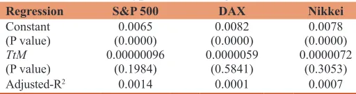
Before exploring the relationships among volatility and our new trading-related variables, we study the fulfillment of the Samuelson hypothesis by estimating a regression of the volatility on the time to maturity (number of days until expiration), for each one of the underlying indexes, see equation (7). For the Samuelson hypothesis to hold, the slope coefficient that accompanies the time-to-maturity variable should be negative.
Table 2 shows that any slope coefficient is, however, not significantly different from zero for our three stock index futures
7 Following their idea, in order to avoid the rollover jump in prices, we calculated the normalized open of the day after the rollover date as the difference between the logarithm of the opening price of that day and the logarithm of the previous closing price of the same contract. The same type of rollover adjustment is followed when computing the absolute change of the open interest. By doing so, all data are taken from the same maturity.
volatility series8. Therefore, in our empirical analysis, it will not be necessary to use a time-to-maturity variable to control for the Samuelson effect.
Now, in order to investigate the relationship between volatility and the flows of entering trades and cancelling trades, we estimate the following regression:
8 Our results are in line with those obtained by Duong and Kalev (2008), who analyse 20 futures contracts, including the S&P 500, and find strong support for the Samuelson hypothesis only for agricultural futures.
Table 1a: Descriptive statistics: Daily stock index futures volatility (in percentage)
Statistics S&P 500 DAX Nikkei
Maximum 4.73 7.03 3.88
Mean 0.68 0.84 0.81
Minimum 0.02 0.10 0.01
Standard deviation 0.43 0.56 0.42
This table reports the maximum, mean, minimum and standard deviation of the daily volatility (times 100) for the S&P 500, DAX and Nikkei index futures, from December 2, 1991 through to April 30, 2008. S&P 500: Standard & Poor 500
Table 1b: Descriptive statistics: Daily stock index futures volume
Statistics S&P 500 DAX Nikkei
Maximum 284.46 537.61 267.44
Mean 83.80 65.62 42.20
Minimum 0.60 1.65 0.17
Standard deviation 42.88 63.25 30.13
This table reports the maximum, mean, minimum and standard deviation of the daily volume (divided by 1,000) for the S&P 500, DAX and Nikkei index futures, from December 2, 1991 through to April 30, 2008. S&P 500: Standard & Poor 500
Table 1c: Descriptive statistics: Daily stock index futures open interest change
Statistics S&P 500 DAX Nikkei
Maximum 8592.89 243.80 58.70
Mean −7.04 −1.71 −2.58
Minimum −8581.59 −380.89 −418.71
Standard deviation 190.42 19.74 23.33
This table reports the maximum, mean, minimum and standard deviation of the daily change in open interest (divided by 1000) for the S&P 500, DAX and Nikkei index futures, from December 2, 1991 through to April 30, 2008. S&P 500: Standard & Poor 500
Table 2: Samuelson hypothesis testing
Regression S&P 500 DAX Nikkei
Constant 0.0065 0.0082 0.0078
(P value) (0.0000) (0.0000) (0.0000)
TtM 0.00000096 0.0000059 0.0000072
(P value) (0.1984) (0.5841) (0.3053)
Adjusted-R2 0.0014 0.0001 0.0007
This table reports the tests of the Samuelson hypothesis for the daily volatility for the S&P 500, DAX and Nikkei index futures, from December 02, 1991 through to
April 30, 2008. The results refer to the regression:VGKYZt= +α βTtMt t+ε, where the
dependent variable,VGKYZt, is the Yang–Zhang extension of the daily Garman-Klass
volatility measure, and the independent variable TtMt is the time to maturity, measured
as the number of days until expiration. P values are given inside parenthesis. The results are obtained with the Newey and West (1987) heteroskedasticity-consistent covariance
procedure. The values of the adjusted-R2 statistics are also reported above. S&P 500:
V V OP OP CL CL
RN
GKYZ
l L
l GKYZ t t t t
t = + t + + + +
+
= − −
∑
−α α β β γ γ
δ
0
1
0 1 1 0 1 1
1
1
O
OP ZERO OP RNOP
CL RNOP
t t t
t t t
(
)
+ ×(
>)
+ ×
(
<)
+δ
δ ε
2
3
95
5
%
%
(8)
By using the following estimation procedure. Firstly, the appropriate number of lags (L) for the volatility variable is determined by a standard time-series methodology: We begin with one lag and check whether its coefficient is significantly different from zero at the 99% level of confidence. If so, we add a new lag to the autoregressive part of the model and then we check the significance of the autoregressive coefficients as well as whether the new model improves in terms of adjusted R2 as well as the Akaike and the Schwarz information criteria. If the coefficients are significantly different from zero and the model improves, we keep the new lag and we continue adding new lags in the same manner. If not, we do not keep it and get the final number of lags. Secondly, we add the seven above-mentioned trading-related variables and we estimate all the coefficients of the whole model. We also compute the adjusted R2, Akaike criterion and Schwarz criterion statistics for the final model. All the regressions have been carried out using the Newey and West correction that accounts for heteroskedasticity and serial correlation9.
9 We checked that our data did not present multicollinearity problems between
the open and closed variables. Specifically, we took the residuals of a regression of closed positions on open positions, which were orthogonal to the open positions variable, and repeated the regression in equation (8) with the residuals instead of the closed positions series. We obtained similar results.
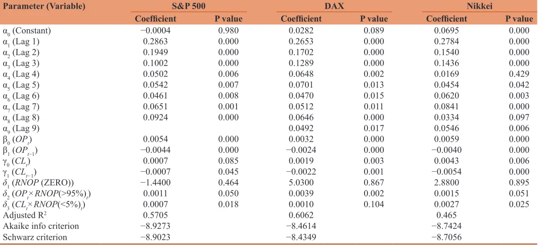
Table 3 reports the estimation results for model (8).
An autoregressive component with eight lags for the volatility is used for the S&P 500 volatility data, while nine lags are employed both for the DAX and Nikkei10.
5.1. Volatility and the Number of Open and Closed Positions
The estimation results reported in Table 3 show that the opening of positions and the closing of positions are both contemporaneously and positively related to volatility in index futures markets (although the absence of a relationship between the contemporaneous number of closed positions and volatility cannot be rejected at the 5% of significance level in the S&P 500 case).
In addition, the lagged numbers of open and closed positions are both related to volatility, for all the indexes. The signs of the coefficients for the contemporaneous (positive) and lagged (negative) open and close variables suggest that the daily change in open and closed positions should be positively related to volatility
10 Fleming et al. (2006) also show the importance of taking into account the persistence in volatility in the analysis of the relationship between volatility and some trading-related variables for 20 stocks traded in the MMI (NYSE). Among the growing evidence that points to stock volatility as a long-memory process we can find, for instance, Andersen et al. (2001), Breidt et al. (1994), and Ding et al. (1993). Nonetheless, Fujihara and Mougoué (1997) show that the introduction of the current and/or lagged volume and open interest substantially reduced the persistence of volatility for oil futures. Similar results are obtained by Wang and Yau (2000) for Deutsche mark, silver and gold futures contracts.
Table 3: Regressions of open and closed positions and RNOP on volatility
Parameter (Variable) S&P 500 DAX Nikkei
Coefficient P value Coefficient P value Coefficient P value
α0 (Constant) −0.0004 0.980 0.0282 0.089 0.0695 0.000
α1 (Lag 1) 0.2863 0.000 0.2653 0.000 0.2784 0.000
α2 (Lag 2) 0.1949 0.000 0.1702 0.000 0.1540 0.000
α3 (Lag 3) 0.1002 0.000 0.1289 0.000 0.1436 0.000
α4 (Lag 4) 0.0502 0.006 0.0648 0.002 0.0169 0.429
α5 (Lag 5) 0.0542 0.007 0.0701 0.013 0.0454 0.042
α6 (Lag 6) 0.0461 0.008 0.0470 0.015 0.0620 0.003
α7 (Lag 7) 0.0651 0.001 0.0512 0.011 0.0841 0.000
α8 (Lag 8) 0.0924 0.000 0.0646 0.000 0.0334 0.097
α9 (Lag 9) 0.0492 0.017 0.0546 0.006
β0 (OPt) 0.0054 0.000 0.0032 0.000 0.0059 0.000
β1 (OPt−1) −0.0044 0.000 −0.0024 0.000 −0.0040 0.000
γ0 (CLt) 0.0007 0.085 0.0019 0.003 0.0043 0.006
γ1 (CLt−1) −0.0007 0.045 −0.0022 0.001 −0.0054 0.000
δ1 (RNOP (ZERO)) −1.4400 0.464 5.0300 0.867 2.8800 0.895
δ2 (OPt×RNOP(>95%)t) 0.0011 0.050 0.0039 0.002 0.0015 0.051
δ3 (CLt×RNOP(<5%)t) 0.0007 0.018 0.0010 0.104 0.0027 0.025
Adjusted R2 0.5705 0.6062 0.465
Akaike info criterion −8.9273 −8.4614 −8.7424
Schwarz criterion −8.9023 −8.4349 −8.7056
This table presents the estimated coefficients together with their associated P values of the regressions on volatility of a constant [α0], the volatility lags [α1,., α9], open positions on day
t and day t−1 [β0, β1], closed positions on day t and day t−1 [γ0, γ1], and RNOP(ZERO)t, OPt×RNOP(>95%) t, and CLt×RNOP(<5%) t, [δ1,δ2,δ3], for the S&P 500, DAX and Nikkei
for all the indexes. Additional regressions confirm that this is in fact the case11.
5.2. Additional Effects for Specific Days
These general relationships may be qualified for those days largely characterized by either the opening of the new positions or the closing of outstanding positions. We now explore these possibilities by the analysis of the coefficients related to the truncated variables that are related to those days with an extreme value of the relative net number of open positions, RNOP, i.e.:
OP × RNOP(>95%) and CL × RNOP(<5%), respectively (recall that whereas the former variable takes the number of open positions whenever the traders are mostly opening positions, the latter takes the number of closed positions whenever the traders are mainly closing previously held positions).
First of all, the estimation results reported in Table 3 for these two variables do not modify the positive sign of the general relationship between volatility and the opening and closing of positions for those days characterized by a large number of contracts entered into or closed out, respectively.
Second, in general, both truncated variables do have a positive relationship with volatility. Additionally, the estimation results for the truncated variable related to RNOP(>95%) show that there is an additional positive effect of the number of open positions
OP for those days in which most positions are newly opened ones (this effect is of marginal significance for the S&P 500 and Nikkei cases). The truncated variable related to RNOP(<5%) also shows that there is an additional positive effect of the number of closing positions CL on those days mostly dominated by closing trades, except for the DAX case, which shows no additional relationship. The result obtained for the variable CL × RNOP(<5%) in the S&P 500 index case is particularly relevant because it shows that the contemporaneous number of closing positions, CLt, has a positive relationship with volatility on those days mostly characterized by the closing of positions for this index, although it did not show a relationship on average when all the days were considered.
Finally, the dummy variable RNOP(ZERO) is not significantly different from zero for any index. This indicates that days largely characterized by a number of opening positions close to the number of closing positions do not have a significantly different volatility on average12.
Overall, our results show that there is a positive relation between the opening of positions and the daily volatility in stock index futures. This positive relation is stronger for those days with a
11 Indeed, we ran a regression similar to (8) where OPt, OPt−1, CLt and CLt−1
were substituted by DOPt (defined as: DOPt = OPt−OPt−1) and DCLt
(defined accordingly). The estimation results showed that both DOPt and
DCLt had a positive relationship with volatility, even for the S&P 500 case (for which the coefficient of CLt was not statistically different from zero at the 5% significance level in the original regression [8]). The estimation results can be obtained from the authors upon request.
12 We also checked for the significance of the truncated variable defined by: (OPt + CLt) × RNOP(ZERO)t, by substituting RNOP(ZERO)t for it in the general regression (8), and also its coefficient was not statistically different from zero.
massive flow of positions entering into the market. Furthermore, there is also a positive relationship between the number of positions being closed and the daily volatility, although there are some differences in this regard among the three indexes. Whereas for the DAX and Nikkei indexes the relation can be observed during the whole sample period (with a stronger positive relationship for days with most traders getting out of the market in the Nikkei case), for the S&P 500 case it concentrates on days largely characterized by the closing of positions.
5.3. Other Aggregated Trading-related Variables
As was previously mentioned, although there is evidence that documents a positive (respectively, negative) relation between trading volume (respectively, lagged volume) and volatility in stock index futures, the sign of the relationship (if any) between open interest and volatility is controversial. A variety of results regarding the significance and the sign of the relationship have been found. Whether this variety of results indicates some sort of genuine difference among stock index futures markets, or it is solely a consequence of methodological discrepancies and/or diverse sample periods, is still unknown.
Fortunately, our results admit a complementary reading in terms of these traditional trading variables (namely, trading volume and open interest) that may help to clarify whether there is indeed any difference among index futures markets, whenever the same methodology and sample period are used to make the comparisons.
Indeed, it is possible to infer the empirical relationships among volatility on one side and trading volume VOL and open interest OI
on the other, from our results, given the accounting relationships that link them to the open OP and close CL variables (both contemporaneously and lagged).
At the end of Appendix A, it is shown that the expression: β0OPt + β1OPt−1 + γ0CLt + γ1CLt−1, contained in the regression (8), can be alternatively written as: [β0 + γ0] VOLt + [β1 + γ1] VOLt−1 + [β0−γ0] ∆OIt + [β1−γ1] ∆OIt−1, in terms of the volume of trading and the change in open interest variables.
The latter expression shows that we can infer the links between volatility and the volume of trading as well as the change in open interest by testing the significance of the sums and subtractions of coefficients that appear inside brackets. For example, a possible contemporaneous relationship between trading volume VOLt and volatility VGKYZt can be explored by testing the null hypothesis: H0: β0 + γ0 = 0, from the coefficients β0 and g0 that appear in the regression (8). The results of these tests are reported in Table 4.
On the other hand, the relation between volatility and open interest depends on the stock index market being explored, even when the same methodology and sample period is used in the analysis. First, neither contemporaneous nor lagged changes in open interest are related to volatility for the cases of the DAX and Nikkei indexes. Second, both contemporaneous and lagged changes in open interest are, however, positively and negatively, respectively, related to volatility for the S&P 500 index case. Furthermore, the signs of the coefficients in this case suggest a positive relationship between the daily variation in the change of open interest and the daily volatility.
5.4. Some Final Comments on Alternative Interpretations
Recall that, in addition to some disagreement on the basic stylized facts, the literature that explores the relationship between volatility, on one side, and trading volume and open interest, on the other, lacks a unifying explanation and some unique interpretation.
Now, our results in Table 4 have shown that the effect of the change in open interest on the volatility is not the same across the three futures markets. Unfortunately, following the line of reasoning that relates volume and open interest to liquidity and depth in futures markets, it is difficult to explain why the relation between volatility and open interest depends on which stock index market is being examined, even when the same methodology and sample period are used in the analysis, as we do in this paper.
However, we also showed previously that our results are consistent for all the indexes, when they are properly interpreted under the perspective offered in this paper: It is the daily changes in the flows of contracts entering and exiting the market that (positively) influence the daily volatility in stock index futures markets. Indeed, we have shown in Table 3 that when open and closed positions are separately considered, only the open positions matter for the S&P 500 index, whereas open positions as well as closed positions both matter for the DAX and Nikkei indexes. Nonetheless, for these two indexes, as the effects of open and closed positions offset each other, the impact of the change in open interest on volatility is null (Table 4).
On the contrary, following the alternative line of reasoning that relates volume and open interest to the trading activity carried out by informed traders (speculators) and uninformed traders (hedgers), Lucia and Pardo (2010) defined the so-called R3 ratio
(RNOP in this paper) as the change in open interest divided by volume, in order to capture the relative importance of the speculation versus hedging activities. As they also pointed out, a value of the ratio close to zero can be associated with intraday and subrogating activities, whereas the two extreme values (namely, −1 and 1) can be allegedly linked to uninformed traders.
Based on these insights, we now provide a possible interpretation of our estimation results based on the relevant values of RNOP, i.e., the variables RNOP(ZERO), RNOP(>95%) and RNOP(<5%). There are two main conclusions that can be extracted from Table 2. Firstly, the coefficients of the RNOP(ZERO) variable are never significantly different from zero, and therefore, we can conclude that a market session fully dominated by intraday and subrogating activities does not increase on average the volatility on that day. This could be the case because both types of activities do not affect volatility, or because the effect of one of them is cancelled out by an opposite effect from the other. Secondly, in general, we observe that when uninformed traders are massively opening (RNOP[>95%]) and closing (RNOP[<5%]) positions in the futures market, they add volatility to such trading day.
6. CONCLUSIONS
A number of papers have analyzed the influence of both the volume and the open interest on index futures volatility. However, there are few stylized facts to be extracted from their diverse results (particularly those related to the open interest). After applying the same methodology to a set of three stock index futures over a 16-year period, our analysis confirms the following general conclusion: Whereas the sign of the correlation between volatility and volume of trading (both contemporaneous and lagged) is the same in all three index futures, the relationship with (the change in) open interest is not.
It is difficult to explain coherently this empirical puzzle. It can be resolved, however, when the evolution of volatility is related to contracting-activity variables (i.e., how new contracts are entered into the market and how outstanding positions are closed out) instead of the volume and open interest variables. Indeed, when open and closed positions are substituted for the traditional variables such as volume and (change in) open interest, the results are essentially the same for all the indexes.
In summary, our results show that, for the three studied stock index futures contracts, in general the number of contemporaneous (respectively, lagged) open positions and closed positions are both positively (negatively) correlated with volatility. Nonetheless, for the S&P 500 case, the relation between the contemporaneous number of closed positions and the volatility is only detected on those days mostly dominated by the closing of positions. Notice that the separated effects of open and closed positions on volatility allow us to provide a consistent story for the importance of the change in the open interest in the analysis. The coherency of our conclusions confirms the empirical relevance of the change in perspective.
Additionally, our results can be reconciled with the line of reasoning that relates volatility to the activity of different groups Table 4: Hypothesis testing
H0 S&P 500 DAX Nikkei
Value P value Value P value Value P value
β(0)+γ(0)=0 0.0060 0.000 0.0051 0.000 0.0102 0.000 β(1)+γ(1)=0 −0.0051 0.000 −0.0046 0.000 −0.0095 0.000 β(0)−γ(0)=0 0.0047 0.000 0.0013 0.285 0.0015 0.586 β(1)−γ(1)=0 −0.0036 0.000 −0.0003 0.813 0.0014 0.398
This table presents the values of the sum (difference) of the coefficients of the variables OP and CL from Table 3 together with the P value of a F-statistic that tests the null
hypotheses, H0, indicated in the first column, for S&P 500, DAX and Nikkei index
of traders, such as speculators, or informed traders versus hedgers, or uninformed traders. According to our findings, intraday and subrogating activities taken together are not associated with a particular increase in volatility. Therefore, intraday traders seem to provide liquidity to the market without destabilizing it. Furthermore, opening and closing positions massively are both connected with a rise in volatility.
7. ACKNOWLEDGMENTS
A version of the paper was presented at the XII Iberian-Italian Congress of Financial and Actuarial Mathematics at Lisbon, Portugal. We thank some congress participants for valuable discussions and comments. We also thank several anonymous referees for useful suggestions. This work was supported by the Spanish Ministerio de Economía y Competitividad and FEDER (under the project ECO2013-40816-P), and the Cátedra Finanzas Internacionales-Banco Santander of the University of Valencia. Finally, we thank Neil Larsen for linguistic advice.
REFERENCES
Andersen, T.G., Bollerslev, T., Diebold, F.X., Ebens, H. (2001), The
distribution of stock return volatility. Journal of Financial Economics, 61, 43-76.
Ap Gwilym, O., Buckle, M., Evans, P. (2002), The Volume-Maturity Relationship for Stock Index, Interest Rate and Bond Futures Contracts. EBMS Working Paper EBMS/2002/3.
Ap Gwilym, O., MacMillan, D., Speight, A. (1999), The intraday
relationship between volume and volatility in LIFFE futures markets.
Applied Financial Economics, 9, 593-604.
Bessembinder, H., Seguin, P. (1993), Price volatility, trading volume, and
market depth: Evidence from futures markets. Journal of Financial and Quantitative Analysis, 28, 21-39.
Breidt, F.J., de Lima, P., Crato, N. (1994), Modeling Long Memory
Stochastic Volatility. Working Papers in Economics. No. 323. Johns Hopkins University.
Carchano, O., Pardo, A. (2009), Rolling over stock index futures contracts.
Journal of Futures Markets, 29, 684-694.
Chen, N.F., Cuny, C.J., Haugen, R.A. (1995), Stock volatility and the
levels of the basis and open interest in futures contracts. Journal of
Finance, 50, 281-300.
Chesney, M., Crameri, R., Mancini, L. (2015), Detecting abnormal
trading activities in option markets. Journal of Empirical Finance, 33, 263-275.
Conrad, J.S., Hameed, A., Niden, C. (1994), Volume and autocovariances
in short-horizon individual security returns. Journal of Finance, 49,
1305-1329.
Ding, Z., Granger, C., Engle, R.F. (1993), A long memory property of
stock market returns and a new model. Journal of Empirical Finance,
1, 83-106.
Duong, H.N., Kalev, P.S. (2008), The Samuelson hypothesis in futures
markets: An analysis using intraday data. Journal of Banking and
Finance, 32, 489-500.
Epps, T.W., Epps, L.M. (1976), The stochastic dependence of security
price changes and transaction volumes: Implications for the
mixture-of-distribution hypothesis. Econometrica, 44, 305-321.
Figlewski, S. (1981), Futures trading and volatility in the GNMA market.
Journal of Finance, 36, 445-456.
Fleming, J., Kirby, C., Ostdiek, B. (2006), Stochastic volatility, trading volume, and the daily flow of information. Journal of Business,
79(3), 1551-1590.
Foster, F.J. (1995), Volume-volatility relationships for crude oil futures
markets. Journal of Futures Markets, 15, 929-951.
Fujihara, R.A., Mougoué, M. (1997), Linear dependence, nonlinear dependence and petroleum futures market efficiency. Journal of
Futures Markets, 17, 75-99.
Fung, H.G., Patterson, G.A. (1999), The dynamic relationship of
volatility, volume, and market depth in currency futures markets. Journal of International Financial Markets, Institutions and Money, 17, 33-59.
Gannon, G.L. (1995), Simultaneous volatility effects in index futures. Review of Futures Markets, 13, 25-44.
Garcia, P., Leuthold, M.R., Zapata, H. (1986), Lead-lag relationships
between trading volume and price variability: New evidence. Journal
of Futures Markets, 6, 1-10.
Garman, M.B., Klass, M.J. (1980), On the estimation of security price
volatilities from historical data. Journal of Business, 53, 67-78.
Jena, S.K., Dash, A. (2014), Trading activity and Nifty index futures
volatility: An empirical analysis. Applied Financial Economics, 24, 1167-1176.
Kawaller, I.G., Koch, P.D., Peterson, J.E. (1994), Assessing the intra-day
relationship between implied and historical volatility. Journal of Futures Markets, 18, 399-426.
Lucia, J.J., Pardo, A. (2010), On measuring speculative and hedging
activities in futures markets from volume and open interest data. Applied Economics, 42, 1549-1557.
Martinez, V., Tse, Y. (2008), Intraday volatility in the bond, foreign
exchange, and stock index futures markets. Journal of Futures Markets, 28, 953-975.
Newey, W., West, K. (1987), Hypothesis testing with efficient method of moment estimation. International Economic Review, 28, 777-787. Parkinson, M. (1980), The extreme value method for estimating the
variance of the rate of return. Journal of Business, 53, 61-65.
Pati, P.C. (2008), The relationship between price volatility, trading volume
and market depth: Evidence from an emerging Indian stock index futures market. South Asian Journal of Management, 15, 25-46.
Poteshman, A. (2006), Unusual option market activity and the terrorist attacks of september 11. Journal of Business, 79, 1703-1726. Ragunathan, V., Peker, A. (1997), Price variability, trading volume and
market depth: Evidence from the Australian futures market. Applied Financial Economics, 7, 447-454.
Ripple, R.D., Moosa, I.A. (2009), The effect of maturity, trading volume,
and open interest on crude oil futures price range-based volatility.
Global Finance Journal, 20, 209-219.
Rogers, L.C.G., Satchell, S.E. (1991), Estimating variance from high, low and closing prices. Annals of Applied Probability, 1, 504-512. Rogers, L.C.G., Satchell, S.E., Yoon, Y. (1994), Estimating the volatility of
stock prices: A comparison of methods that use high and low prices. Applied Financial Economics, 4, 241-47.
Schwert, G.W. (1989), Why does stock market volatility change over
time. Journal of Finance, 44, 1115-1153.
Schwert, G.W. (1990), Stock market volatility. Financial Analysts Journal,
46, 23-34.
Smirlock, M., Starks, L. (1985), A further examination of stock price changes and transactions volume. Journal of Financial Research,
8, 217-225.
Susheng, W., Zhen, Y. (2014), The dynamic relationship between volatility, volume and open interest in CSI 300 futures market. WSEAS Transactions on Systems, 13, 1-11.
Wang, C. (2002), The effect of net positions by the type of trader on
volatility in foreign currency futures markets. Journal of Futures
Markets, 22, 427-450.
volatility in futures markets. Journal of Futures Markets, 20, 943-970. Watanabe, T. (2001), Price volatility, trading volume, and market depth:
Evidence from the Japanese stock index futures market. Applied
Financial Economics, 11, 651-658.
Yang, D., Zhang, Q. (2000), Drift-independent volatility estimation based
on high, low, open, and close prices. Journal of Business, 73, 477-491.
Every trade involves two parties (long and short) and each party either opens or closes out a position. Hence, the total number of open and closed positions equals the total number of positions involved in the traded contracts (i.e., twice the number of traded contracts):
OPt + CLt = 2Vt (A.1)
Furthermore, the sum of all the open positions from the first trading day of the contract up to the end of day t minus the sum of all the closed positions up to the same moment must be equal to the total number of outstanding (long plus short) positions at the end of day
t (i.e. twice the open interest at the same moment), that is:
s t
s s t
OP CL OI
=
∑
(
−)
=1
2 (A.2)
From equation (A.2), it follows that:
OPt−CLt = 2ΔOIt (A.3)
Where, ∆OIt = OIt−OIt−1. It is important to notice that although OIt is a stock variable measured at the end of day t, the change in open interest over day t, ΔOIt, is a flow variable, just like the trading volume, which only depends on the behavior of traders on the observation day.
Now, from equations (A.1) and (A.3), the following accounting relationships can be easily obtained:
OPt = VOLt + ΔOIt (A.4)
CLt = VOLt−ΔOIt (A.5)
(These are equations (1) and (2) in the main body of the paper.)
If we define the relative net number of open positions on day t, RNOPt, as in equation (3), i.e.:
RNOPt = (OPt−CLt)/(OPt + CLt) (A.6)
It can be easily checked that RNOPt equals ∆OIt/VOLt. This shows that RNOP coincides with the so-called R3 ratio introduced by Lucia and Pardo (2010) in the context of a critical assessment of the literature devoted to measuring the hedging activity from volume and open interest data. They pointed out that RNOP (or R3 as they called it) can only take values in the range [–1, +1]. Lucia and Pardo (2010) also pointed out that RNOP (R3) equals zero whenever every trade is a day-trade or it implies that one side involved in the trade replaces the other side in a previous position.
Finally, from equations (A.1) and (A.6), we can also get:
OPt = VOLt (1 + RNOPt) (A.7)
CLt = VOLt (1−RNOPt) (A.8)
(These are equations (4) and (5) in the paper.)
In addition, the mathematical expression: β0OPt + β1OPt−1 + γ0CLt + γ1CLt−1, where β0, β1, γ0 and γ1 are constant parameters, can be written, from equations (A.4) and (A.5), as: β0 [VOLt + ∆OIt] + β1 [VOLt−1 + ∆OIt−1] + γ0 [VOLt−∆OIt] + γ1 [VOLt−1−∆OIt−1], which in turn can be finally reordered as: [β0 + γ0] VOLt + [β1 + γ1] VOLt−1 + [β0−γ0] ∆OIt + [β1−γ1] ∆OIt−1.
APPENDIX B
Following the assumptions of Garman and Klass (1980), Parkinson (1980), Rogers and Satchell (1991), Rogers et al. (1994), and Yang and Zhang (2000) make explicit the following formula for the efficient (minimum-variance) drift-independent unbiased estimator of Garman and Klass for the variance of a financial series, based on n observations during a given observation period:
VGKYZ =Vo'− Vc'+ VP+ VRS
. . .
0 383 1 364 0 019 (B.1)
Where, Vo' and V
c' are defined as:
Vo n o
i n
i '
/
=
( )
=
∑
11
2 (B.2)
Vc n c
i n
i '
/
=
( )
=
∑
11
2 (B.3)
And Vp (Parkinson, 1980) and VRS(Rogers and Satchell, 1991) are defined as:
VP n u d
i n
i i
=
( )
(
−)
=
∑
1 1
4 2
1
2
/
ln (B.4)
VRS n u u c d d c
i n
i i i i i i
=
( )
(
−)
+(
−)
=
∑
11
/ (B.5)
Where:
oi = ln(Oi)−ln(Ci−1), is the so-called normalized open,
ci = ln(Ci)−ln(Oi), is the normalized close,
ui = ln(Hi)−ln(Oi), is the normalized high And
di = ln(Li)−ln(Oi), is the normalized low.