J. Math. Comput. Sci. 7 (2017), No. 1, 39-58 ISSN: 1927-5307
NUMERICAL SOLUTION OF HAMMERSTEIN INTEGRAL EQUATION USING CHEBYSHEV WAVELET METHOD
J. IQBAL∗, R. ABASS
Department of Mathematical Sciences, BGSB University, Rajouri-185234, J and K, India
Copyright c2017 J. Iqbal and R. Abass. This is an open access article distributed under the Creative Commons Attribution License, which permits unrestricted use, distribution, and reproduction in any medium, provided the original work is properly cited.
Abstract. The aim of this work is to solve Hammerstein integral equations of both Fredholm as well as Volterra type by Chebyshev wavelet method which is widely applicable in engineering and technology. The Chebyshev wavelets together its properties are used to converts the problem into algebraic equations. Illustrative examples of Hammerstein type equations have been discussed to demonstrate the validity and applicability of the technique and the results have been compared with the existing method in the literature as well as with exact solution. Keywords:Chebyshev wavelet; operational matrix of integration; product operational matrix; Hammerstein inte-gral equations; MATLAB.
2010 AMS Subject Classification:45B05, 47G20, 65T60.
1. Introduction
Many problems of mathematical physics can be stated in the form of integral equations. These equations also occur as reformulations of other mathematical problems such as partial differential equations and ordinary differential equations. The study of integral equations and
∗Corresponding author
Received September 2, 2016
methods for solving them are very useful in many fields including many problems in mathemat-ical physics, the dynamic model of chemmathemat-ical reactor, problems in control theory, and various reformulations of an elliptic partial differential equation with nonlinear boundary conditions. In this paper, we consider the nonlinear Fredholm-Hammerstein integral equations and nonlinear Volterra-Hammerstein integral equations respectively by the general forms [1, 13]
y(t) = f(t) +λ
Z 1
0
K(t,x)F(x,y(x))dx, (1.1)
y(t) = f(t) +λ
Z t
0
K(t,x)F(x,y(x))dx, (1.2)
where the parameterλ and functions f(t),K(t,x)andF(x,y(x))∈L2[0,1]are known
Over the last couple of decades, wavelets have been studied extensively and have emerged as a powerful computational tool for attaining numerical solutions for a wide range of prob-lems including integral, algebraic, differential, partial-differential, functional-delay and integro-differential equations. Wavelets are calculated as continuously oscillatory functions and pos-sess attractive features: zero-mean, fast decay, short life, time-frequency representation, multi-resolution, etc. Wavelets have the ability to detect information at different scales and at different locations throughout a computational domain. Wavelets can provide a basis set in which the ba-sis functions are constructed by dilating and translating a fixed function known as the mother wavelet. The wavelet method allows the creation of very fast algorithms when compared with the algorithms ordinarily used. Wavelets are considerably useful for solving Fredholm cum Volterra Hammerstein integral equations and provide accurate solutions.
In recent years, different types of wavelets and approximating functions based on orthogo-nal functions have been used to approximate the numerical solution of integral and differential equations such as Chebyshev [24], Legendre [2, 10], Daubechies [20], Alpert [12], Modifed Homotopy Perturbation [7] and Haar [17] wavelets. Among all the wavelet families, the Cheby-shev wavelets have gained popularity among researchers due to their useful properties such as simple applicability, orthogonality and compact support. The main characteristic of Chebyshev wavelet is that it converts the problems into nonlinear system of algebraic equations and this system may be solved by using an appropriate numerical method. This approach used opera-tional matrixPof integration and product operation matrix to eliminate the integral operator. The rest of the paper is as follows: In section 2, Chebyshev wavelet, its properties, function approximations and convergence are discussed. Operational Matrix of Integration(OMI) is pre-sented in section 3. In section 4, product operation matrix of Chebyshev wavelets have been discussed. Section 5, is devoted to present a computational method for solving Hammerstein in-tegral equations utilizing Chebyshev wavelets and approximate the unknown function. Section 6, deals with the illustrative examples and their solutions by the proposed approach compared with exact as well as with existing literature. Finally, we conclude the article in section 7.
Wavelets constitute the family of functions constructed from the dilation and translation of a single function known as the Mother wavelet. When the dilation parameter a and translation parameterbvary continuously we have the following family of continuous wavelets [8]
ψa,b(t)=|a|−
1 2ψ
t−b a
; a, b ∈R, a6=0. (2.1)
If we choosea=a−kandb=nba−kwherea>1,b>0 andn,k∈Z+then we get the following family of discrete wavelets:
ψk,n(t) =|a|− k
2ψ(akt−nb). (2.2)
These family of functions are a wavelet basis forL2(R)and makes an orthonormal basis for the special casea=2 andb=1.
Chebyshev waveletsψn,m(t) =ψ(k,m,n,t)have four arguments,k=0,1,2, ...,n=1,2, ...,2k,m is the degree of Chebyshev polynomial of first kind andt denotes the normalized time. They are defined on the interval[0,1)by
ψn,m(t) =
αm√2k/2
π Tm(2
k+1t−2n+1), n−1 2k ≤t≤
n
2k
0, otherwise
(2.3)
where
αm=
√
2, m=0
2, m=1,2, . . .
Tm(t) in (2.3) are well known Chebyshev polynomial of order m, which is orthogonal with respect to the weight functionω(t) = √1
1−t2 and satisfy the following recursive formula:
T0(t) =1
T1(t) =t
Moreover, the set of Chebyshev wavelet are an orthogonal set with respect to the weight func-tionωn(t) =ω(2k+1t−2n+1).
A function f(t)∈L2[0,1]may be expanded as
f(t) = ∞
∑
n=1
∞
∑
m=0
cnmψnm(t), (2.4)
where the wavelet coefficients of the series representation in (2.4) become
cnm=hf(t),ψnm(t)iwn(t). (2.5)
The convergence of the series (2.4), inL2[0,1], means that
lim s1,s2→∞
f(x)−
s1
∑
n=1
s2
∑
m=0
cnmψnm(t)
=0.
If the infinite series in(2.4)is truncated then equation(2.4)can be written as
f(t)∼=
2k−1
∑
n=1
M−1
∑
m=0
cnmψnm(t) =CTΨ(t), (2.6)
whereCandΨ(t)are 2k−1M×1 matrices given by:
C= [c1,0,c1,1, . . . ,c1,M−1,c2,0,c2,1, . . . ,c2,M−1, . . . ,c2k−1,0, . . . ,c2k−1M−1]T, (2.7)
Ψ(t) = [ψ1,0,ψ1,1, . . . ,ψ1,M−1,ψ2,0,ψ2,1, . . . ,ψ2,M−1, . . . ,ψ2k−1,0, . . . ,ψ2k−1,M−1]T. (2.8)
In the same way, a function of two variableK(x,t)∈L2([0,1]×[0,1])may be approximated as:
K(x,t)≈ΨT(x)KΨ(t), (2.9)
whereKis 2k−1M×2k−1Mmatrix, withKi j = (ψi(x),(K(x,t),ψj(t))).
The integration of the product of two Chebyshev wavelets vector functions with respect to the weight functionWn(t), is derived as
Z 1
0
whereI is the identity.
Also the integer powers of a function may be approximated as
[y(t)]p= [YTΨ(t)]p=Yp∗TΨ(t), (2.11)
whereYp∗ is a 2k−1×1 matrix, whose elements are nonlinear combinations of the elements of the vectorY.Yp∗is called the operational vector for production of thepth power of the function
y(t)[3, 8, 18].
Since the truncated Chebyshev wavelets series can be an approximate solution of singular inte-gral equations, one has an error functionE(t)for f(t)as follows:
E(t) =f(t)−CTΨ(t) .
3. Operational Matrix of Integration(OMI)
In this section, we will first derive the operational matrixPof integration [21, 22, 24] which help us in dealing with the concerned problems Hammerstein integral equations . First we construct the matrixPfork=2 andM=3. In this case, the six basis functions are given by
ψ1,0= √2π,
ψ1,1= 2
q
2
π(4t−1),
ψ1,2= 2
q
2
π (4t−1)
2−1
fort∈[0,1/2), (3.1)
ψ2,0= √2π,
ψ2,1= 2
q
2
π(4t−3),
ψ2,2= 2
q
2
π (4t−3)
2−1
By integrating the above defined basis (3.1) and (3.2) from 0 totand using wavelet coefficient, we obtain
Z t
0
ψ1,0(t)dt =
2 √
πt, t∈[0,
1 2)
1
√
πt, t∈(
1 2,1]
=
1 4,
1 4√2,0,
1 2,0,0
T
Ψ6(t),
Z t
0
ψ1,1(t)dt =
2q√2
π, t∈[0,
1 2)
0, t∈(12,1]
=
− 1 8√2,0,
1
16,0,0,0
T
Ψ6(t),
Z t
0
ψ1,2(t)dt=
2q√2
π, 32
3t
3−8t2+t
t∈[0,12)
−13q2
π, t∈(
1 2,1]
=
− 1 6√2,−
1 8,0,−
1 3√2,0,0
T
Ψ6(t),
Z t
0
ψ2,0(t)dt =
0, t∈[0,12)
2
√
πt−
1
π, t∈(
1 2,1]
=
0,0,0,1 4,
1 4√4,0
T
Ψ6(t),
Z t
0
ψ2,1(t)dt =
0, t∈[0,12)
2
q
2 π(2t
2−3t) +1, t∈(1 2,1]
=
0,0,0,− 1
8√2,0,− 1 16
T
Ψ6(t),
Z t
0
ψ2,2(t)dt=
0, t∈[0,12)
2 q 2 π 32 3t
3−24t2+17t−23 6
, t∈(12,1] =
0,0,0,− 1 6√2,−
1 8,0
T
Ψ6(t).
Z t
0
Ψ(t)dt =PΨ(t), (3.3)
wherePis the 2k−1M×2k−1Moperational matrix of integration [3, 4] determined as follows.
P6×6= 1 4
1 √1
2 0 2 0 0
− 1
2√2 0
1
4 0 0 0
−
√
2
3 −
1
2 0 −
2√2
3 0 0
0 0 0 1 √1
2 0
0 0 0 − 1
2√2 0
1 4
0 0 0 −
√ 2 3 − 1 2 0 . (3.4)
For general case, we have
P2k−1M×2k−1M = 1 2k
L F F . . . F
O L F . .. ... O O L . .. F
..
. . .. ... ... F O . . . O O L
, (3.5)
whereL,F andOareM×Mmatrices given by
L= 1 2 1
2√2 0 0 . . . 0 0 0
− 1
8√2 0
1
8 0 . . . 0 0 0
− 1
6√2 −
1
4 0
1
12 . . . 0 0 0
..
. ... ... ... . .. ... ... ...
−√ 1
2(M−1)(M−3) 0 0 0 . . . − 1
4(M−3) 0 −
1 4(M−1)
− 1
2√2M(M−2) 0 0 0 . . . 0 − 1
4(M−2) 0
F=
√
2 0 0 . . . 0 0 0 0 . . . 0 −
√
2
3 0 0 . . . 0
0 0 0 . . . 0 −
√
2
15 0 0 . . . 0
..
. ... ... . .. ... −
√
2
M(M−2) 0 0 . . . 0
and
O=
0 0 . . . 0 0 0 . . . 0
..
. ... . .. ... 0 0 . . . 0
.
4. Product Operation Matrix of Chebyshev Wavelets
The following properties of the product of two Chebyshev wavelet function vectors is also used for solving differential a well as integral equations:
CTΨ(t)ΨT(t)≈C˜ΨT(t), (4.1)
where C and Ψ(t) are give in Eq.(2.7) and (2.8), respectively and ˜C is (2k−1M)×(2k−1M)
Ψ(t)ΨT(t) =
ψ10ψ10 ψ10ψ11 ψ10ψ12 ψ10ψ20 ψ10ψ21 ψ10ψ22
ψ11ψ10 ψ11ψ11 ψ11ψ12 ψ11ψ20 ψ11ψ21 ψ11ψ22
ψ12ψ10 ψ12ψ11 ψ12ψ12 ψ12ψ20 ψ12ψ21 ψ12ψ22
ψ20ψ10 ψ20ψ11 ψ20ψ12 ψ20ψ20 ψ20ψ21 ψ20ψ22
ψ21ψ10 ψ21ψ11 ψ21ψ12 ψ21ψ20 ψ21ψ21 ψ21ψ22
ψ22ψ10 ψ22ψ11 ψ22ψ12 ψ22ψ20 ψ22ψ21 ψ22ψ22
. (4.2)
As we know, the support ofψm,n, the entries of vectorΨ(t)are the intervals
n−1 2k ,
n
2k
, there-foreψi jψkl=0 ifi6=k.We also have
ψi0ψi j= √2πψi j,
ψi1ψi1= √2 πψi0+
q
2 π ψi2.
If we retain only the elements ofΨ(t), then we have
Ψ(t)ΨT(t) =√1
π
2ψ10 2ψ11 2ψ12 0 0 0
2ψ11 2ψ10+
√ 2ψ12
√
2ψ11 0 0 0
2ψ12
√
2ψ11 2ψ10 0 0 0
0 0 0 2ψ20 2ψ21 2ψ22
0 0 0 2ψ21 2ψ20+
√ 2ψ22
√ 2ψ21
0 0 0 2ψ22
√
2ψ21 2ψ22
Therefore the 6×6 matrix ˜Cin Eq.(4.1) can be written as
˜
C=
B1 0
0 B2
, (4.3)
whereBi, i=1,2,are 3×3 matrices given by
Bi= √1
π
2ci0 2ci1 2ci2
2ci1 2ci0+√2ci2 √2ci1
2ci2 √2ci1 2ci0
, (4.4)
whereci,d,d=0,1,2 taken from Eq.(2.7).
For general case, ˜Cis a 2kM×2kM matrix in the form as
˜
C=
B1 0 . . . 0
0 B2 . . . 0 ..
. ... . .. ... 0 0 . . . B2k
, (4.5)
forBi,i=1,2, . . . ,2k taken from Eq.(4.4).
5. Description of the Proposed Method
In this section, we will use the operational matrix of integration and product operation matrix of Chebyshev wavelets to solve Hammerstein integral equation of Fredholm and Volterra type. Firstly, we consider Fredholm Hammerstein integral equation as:
y(t) = f(t) + Z 1
0
where f ∈L2[0,1],K ∈ L2([0,1]×[0,1])andyis an unknown function [6] and p∈Z+. Now we approximate f(t),y(t),k(t,x)and[y(t)]pin the following way:
f(t)'Ψ(t)TF y(t)'Ψ(t)TY, (5.2)
K(t,x)'Ψ(t)TKΨ(t)and [y(t)]p'Ψ(t)TY∗, (5.3)
whereY∗is a column vector function of the elements of the vectorY [3, 4, 18].
By substituting the approximation function mentioned in Eq.(5.2) and Eq.(5.3) into Eq.(5.1) we obtain
Ψ(t)TY=Ψ(t)TF+
Z 1
0
ΨT(t)KΨ(x)ΨT(x)Y∗dx
=Ψ(t)TF+ΨT(t)K
Z 1
0
Ψ(x)Ψ(x)dx
Y∗
=Ψ(t)T(F+KY∗),
then the required non-linear system of algebraic equation become
Y−KY∗=F. (5.4)
Secondly, we consider the following Volterra Hammerstein type integral equation
y(t) = f(t) + Z t
0
K(t,x)[y(x)]pdx, (5.5)
In the light of (4.1),(5.2) and (5.3) we have:
Z t
0
K(t,x)[y(x)]pdx∼= Z t
0
Ψ(t)TKΨ(x)TY∗dx
=ΨT(t)K
Z t
0
Ψ(x)ΨT(x)Y∗dx
=ΨT(t)K
Z t
0
˜
Y∗TΨ(x)dx
Then
ΨT(xi)Y = f(t) +ΨT(t)KY˜∗TPΨ(t). (5.6)
By evaluating this equation in 2k−1Mpoints{ti}2k−1M
i=1 in the interval[0,1]we have a system of
nonlinear equations:
ΨT(xi)Y =F(ti) +ΨT(ti)KY˜∗TPΨ(ti),i=1,2, . . . ,2k−1M. (5.7)
The nonlinear system of algebraic equations (5.4) and (5.7) can be solve by Newton’s methods using mathematical software MATLAB.
6. Numerical experiments and discussion
In this section, we implement the proposed method for solving Hammerstein integral equation to achieve the effectiveness, the validity, the accuracy and support our theoretical discussion in the above sections. we consider four examples of Hammerstein integral equation of Fredohlm and Volterra type. All computations have been done with the software package MATLAB 2013a. The numerical results achieved by the proposed method are shown in Table 6.1-6.4 and graphically shown in Figure 6.1-6.4.
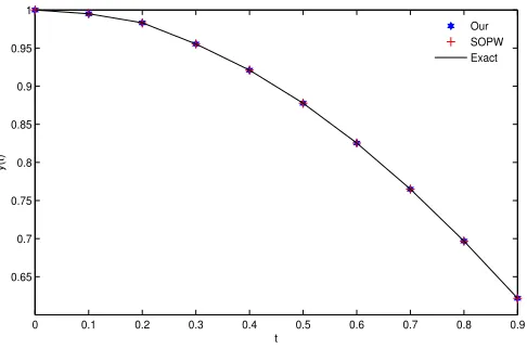
Example 6.1Consider the Fredholm Hammerstein integral of second kind as [5]
y(t) = f(t) + Z 1
0
K(t,x)[y(x)]2dx, 0≤t≤1, (6.1) where
f(t) =1+3 sin2(t) and K(t,x) =
−3 sin(t−x), forx∈[0,1]
0, forx∈[t,1].
Table 6.1: Comparison of the approximate solution of Example 6.1 with exact and the Ref.[15] at different scales.
t OurResult OurResult Re f.[15] Exact
(k=2,M=3) (k=2,M=4) (M=4)
0.0 1.000000 1.000000 1.000000 1.000000
0.1 0.995204 0.995008 0.995012 0.995004
0.2 0.983211 0.983086 0.983077 0.983095
0.3 0.955495 0.955329 0.955324 0.955336
0.4 0.921190 0.921064 0.921066 0.921061
0.5 0.877698 0.877579 0.877575 0.877583
0.6 0.825426 0.825339 0.825343 0.825336
0.7 0.765012 0.764855 0.764859 0.764842
0.8 0.696884 0.696701 0.696694 0.696707
0.9 0.621803 0.621611 0.621603 0.621619
0 0.1 0.2 0.3 0.4 0.5 0.6 0.7 0.8 0.9
0.65 0.7 0.75 0.8 0.85 0.9 0.95 1
t
y(t)
Our SOPW Exact
Fig.6.1Comparison of Exact Solution with Approximate Solution and Ref.[15] for Example 6.1 atk=2,M=4.
y(t) = f(t) + Z 1
0
K(t,x)[y(x)]3dx, 0≤t≤1, (6.2)
where
f(t) =et−(1+2e
3)t
9 andK(t,x) =tx,
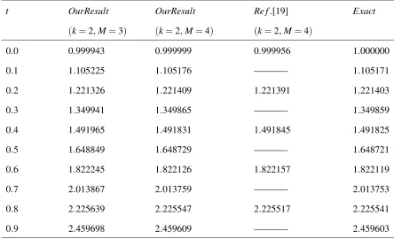
with exact solutiony(t) =et. Table 6.2 and Figure 6.2 show the numerical results for Example 6.2 in comparison with wavelet Glaerkin methods [19].
Table 6.2: Comparison of the approximate solution of Example 6.2 with exact and the Ref.[19] at different scales.
t OurResult OurResult Re f.[19] Exact
(k=2,M=3) (k=2,M=4) (k=2,M=4)
0.0 0.999943 0.999999 0.999956 1.000000
0.1 1.105225 1.105176 ———– 1.105171
0.2 1.221326 1.221409 1.221391 1.221403
0.3 1.349941 1.349865 ———– 1.349859
0.4 1.491965 1.491831 1.491845 1.491825
0.5 1.648849 1.648729 ———– 1.648721
0.6 1.822245 1.822126 1.822157 1.822119
0.7 2.013867 2.013759 ———– 2.013753
0.8 2.225639 2.225547 2.225517 2.225541
0.9 2.459698 2.459609 ———– 2.459603
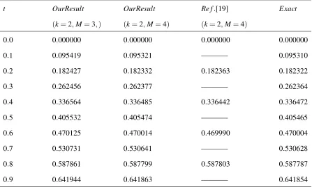
Example 6.3Consider the Volterra Hammerstein integral of second kind [19]
y(t) = f(t) + Z t
0
K(t,x)[y(x)]2dx, 0≤t≤1, (6.3)
where
f(t) =
1−11 9 t+
2 3t
2−1
3t
3−2
9t
4
In(t+1)−1 3(t+t
3)(In(t+1))2−11
9 t
2+ 5
18t
3− 2
27t
0 0.1 0.2 0.3 0.4 0.5 0.6 0.7 0.8 0.9 0.8
1 1.2 1.4 1.6 1.8 2 2.2 2.4 2.6
t
y(t)
Our Exact
Fig.6.2Approximate solution for Example 6.2 atk=2,M=4 with exact solution.
andK(t,x) =tx2with exact solutiony(t) =In(t+1).The numerical results of Example 6.3 are presented in Table 6.3 at different scale and graphically shown in Figure 6.3 atk=2,M=4.
Table 6.3Comparison of the approximate solution of Example 6.3 with exact and the Ref.[19] at different scales.
t OurResult OurResult Re f.[19] Exact
(k=2,M=3,) (k=2,M=4) (k=2,M=4)
0.0 0.000000 0.000000 0.000000 0.000000
0.1 0.095419 0.095321 ———– 0.095310
0.2 0.182427 0.182332 0.182363 0.182322
0.3 0.262456 0.262377 ———– 0.262364
0.4 0.336564 0.336485 0.336442 0.336472
0.5 0.405532 0.405474 ———– 0.405465
0.6 0.470125 0.470014 0.469990 0.470004
0.7 0.530731 0.530641 ———– 0.530628
0.8 0.587861 0.587799 0.587803 0.587787
0.9 0.641944 0.641863 ———– 0.641854
0 0.1 0.2 0.3 0.4 0.5 0.6 0.7 0.8 0.9 0
0.1 0.2 0.3 0.4 0.5 0.6 0.7
t
y(t)
Our Exact
Fig.6.3Approximate solution for Example 6.3 atk=2,M=4 with exact solution.
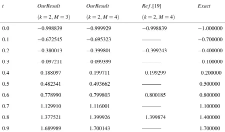
y(t) = f(t) + Z t
0
K(t,x)[y(x)]3dx, 0≤t≤1, (6.4)
where
f(t) = 116 3 e
2t−
116
3 +39t+18t
2+9t3
et+3t−1
and
K(t,x) =−1 3e
2t−x
with exact solutiony(t) =3t−1.
t OurResult OurResult Re f.[19] Exact
(k=2,M=3) (k=2,M=4) (k=2,M=4)
0.0 −0.998839 −0.999929 −0.998839 −1.000000
0.1 −0.672545 −0.695323 ———– −0.700000
0.2 −0.380013 −0.399801 −0.399243 −0.400000
0.3 −0.097211 −0.099399 ———– −0.100000
0.4 0.188097 0.199711 0.199299 0.200000
0.5 0.482341 0.493662 ———– 0.500000
0.6 0.778990 0.799803 0.800185 0.800000
0.7 1.129910 1.116001 ———– 1.100000
0.8 1.377521 1.399926 1.399874 1.400000
0.9 1.689989 1.700143 ———– 1.700000
Table 6.4Comparison of the approximate solution of Example 6.4 with exact and the Ref.[19] at different scales.
0 0.1 0.2 0.3 0.4 0.5 0.6 0.7 0.8 0.9
−1 −0.5 0 0.5 1 1.5 2
t
y(t)
Our Exact
7. Conclusion
In this paper, we have proposed an efficient and accurate method based on Chebyshev wavelets to solve both Fredholm and Volterra Hammerstein integral equations arising in different field of sciences, engineering and technology. Comparisons between our approximate solutions of the problems with its exact solutions and with the approximate solutions achieved by other methods were introduced to confirm the validity and accuracy of our scheme. The numerical experiments confirm that the Chebyshev wavelet method is superior to other existing ones and is highly accurate and can be applicable to Hammerstein integral equation. The main advantage of this Chebyshev wavelet method is that it transfers the whole scheme into a system of algebraic equations for which the computation is easy and simple. In addition, other pretty features of this scheme are its simplicity, applicability and less computational effort.
Conflict of Interests
The authors declare that there is no conflict of interests.
REFERENCES
[1] S. Abbasbandy, Numerical solution of integral equation: Homotopy perturbation method and Adomians decomposition method, Appl. Math. Comput. 173 (2006), 493-500.
[2] H. Adibi, P. Assari, On the numerical solution of weakly singular Fredholm integral equations of the second kind using Legendre wavelets, J. Vib. Control. 17 (2011), 689-698.
[3] E. Babolian, F. Fattahzadeh, Numerical computation method in solving integral equations by using Cheby-shev wavelet operational matrix of integration, Appl. Math. Comp. 188(2007), 1016-1022.
[4] E. Babolian, F. Fattahzadeh, Numerical solution of differential equations by using Chebyshev wavelet oper-ational matrix of integration, Appl. Math. Comp. 188 (2007), 417-426.
[5] H. Brunner, Implicitly linear collocation methods for nonlinear Volterra equations, Appl.Numer. Math. 9(3-5) (1992), 235-247.
[6] L.M. Delves and J.L. Mohammed, Computational methods for integral equatos, Cambridge university press, Oxford, 1983.
[7] A. Golbabai, M. Javidi, Modifed Homotopy Perturbation method for solving non-linear Fredholm integral equations, Chaos. Sols. Fract. 40 (2009), 1408-1412.
[9] G. Q. Han, Asymptotic error expansion of a collocation-type method for Volterra-Hammerstein integral equa-tions, Appl. Numer. Math, 13(5) (1993), 357-369.
[10] S. Javadi, J.Saeidian and F. Safari, Legendre wavelet method for solving Hammerstein integral equations of the second kind. Theo. Appr. Appl. 9(2) (2013), 37-55.
[11] M. T. Kajani, A. H. Vencheh, and M. Ghasemi, The Chebyshev wavelets operational matrix of integration and product operation matrix, Int. J. Comp. Math. 86 (2009), 1181-1125.
[12] H. Kaneko, R. D. Noren, B. Novaprateep, Wavelet applications to the Petrov-Galerkin method for Hammer-stein equations, Appl. Numer. Math. 45 (2003), 255-273.
[13] R. P. Kanwal. Linear integral equations theory and technique, Academic Press; New York and London. 1971. [14] K. Kumar, I. H. Sloan, A new collocation-type method for Hammerstein integral equations, Math. Comp.
48(178) (1987), 585-593.
[15] M. Lakestani, M. Razzagi, M. Dehghan, Solution of nonlinear Fredholm-Hammerstein integral equations by using semiorthogonal spline wavelets, Math. Prob. Engi. 1 (2005), 113-121.
[16] L. J. Lardy, A variation of Nystr¨om’s method for Hammerstein equations, J. Integ. Eqs. 3 (1981), 43-60. [17] U. Lepik, E. Tamme, Solution of nonlinear Fredholm integral equations via the Haar wavelet method, Proc.
Estonian Acad. Sci. Phys. Math. 56 (2007), 17-27.
[18] Y. LI, Solving a nonlinear fractional differential equation using Chebyshev wavelets, Comm. Non. Sci. Num. Simu. 15 (2010), 2284-2292.
[19] Y. Mahmoudi, Wavelet Galerkin method for numerical solution of nonlinear integral equation, Appl. Math. Comp. 167 (2005), 1119-1129.
[20] K. Maleknejad, H. Derili, The collocation method for Hammerstein equations by Daubechies wavelets, Appl. Math. Comput. 172 (2006), 846-864.
[21] M. Razzaghi, S. Yousefi, The Legendre wavelets operational matrix of integration, Int. J. Syst. Sci. 32 (2001), 495-502.
[22] M. Razzaghi, S. Yousefi, Legendre wavelets method for the solution of nonlinear problems in the calculus of variations, Mathematical and Computer Modelling 34 (2001), 45-54.
[23] F. G. Tricomi, Integral Equations, Dover Publications, New York, 1985.