Recommender System
Cr´ıcia Z. Fel´ıcio1,2, Kl´erisson V. R. Paix˜ao2, Guilherme Alves2, Sandra de Amo2, Philippe Preux3 1 Federal Institute of Triˆangulo Mineiro, Brazil
cricia@iftm.edu.br
2 Federal University of Uberlˆandia, Brazil
{klerisson, guilhermealves, deamo}@ufu.br
3 University of Lille & CRIStAL, France
philippe.preux@inria.fr
Abstract. There has been an explosion of social approaches to leverage recommender systems, mainly to deal with cold-start problems. However, most of the approaches are designed to handle explicit user’s ratings. We have envisioned Social PrefRec, a social recommender that applies user preference mining and clustering techniques to incorporate social information on the pairwise preference recommenders. Our approach relies on the hypothesis that user’s preference is similar to or influenced by their connected friends. This study reports experiments evaluating the recommendation quality of this method to handle the cold-start problem. Moreover, we investigate the effects of several social metrics on pairwise preference recommendations. We also show the effectiveness of our social preference learning approach in contrast to state-of-the-art social recommenders, expanding our understanding of how contextual social information affects pairwise recommenders.
Categories and Subject Descriptors: H.3.3 [Information Storage and Retrieval]: Clustering-Information filtering; J.4 [Computer Applications]: Social and behavioral sciences
Keywords: Pairwise Preferences, Social Network, Social Recommender System
1. INTRODUCTION
Social recommender (SR) could shatter the barriers for users to consume information. Thus, there has been an explosion of social approaches in this context [Tang et al. 2013], mainly to deal with cold-start problems. Typical SR systems assume a social network among users and make recommendations based on the ratings of the users who have direct or indirect social relations with the target user [Jamali and Ester 2010]. However, explicit user’s ratings may not capture all the user’s interests without loss of information [Balakrishnan and Chopra 2012]. Pairwise preference learning shows clear utility to tackle such problem [de Amo and Ramos 2014]. The “marriage” between pairwise preference recommender and social network can be used in a unique manner to enhance the recommender effectiveness.
In such way, we advance earlier work,PrefRec[de Amo and Oliveira 2014], a model-based hybrid
recommender system framework based on pairwise preference mining and preferences aggregation techniques. We proposeSocial PrefRec, an approach to incorporate social networks information in
recommendation task to minimize user cold-start problem. Different factors of social relationships have influence on users. Some of these factors contribute or even harm social recommender systems
C. Z. Fel´ıcio would like to thank Federal Institute of Triˆangulo Mineiro for study leave granted. K. V. R. Paix˜ao and G. Alves are sponsored by scholarships from CAPES. We also thank the Brazilian research agencies CAPES, CNPq and FAPEMIG for supporting this work. Ph. Preux’ research is partially funded by Contrat de Plan ´Etat R´egion Data, and the French Ministry of Higher Education and Research, and CNRS; he also wishes to acknowledge the continual support of Inria, and the exciting intellectual environment provided by SequeL.
[Yuan et al. 2015]. Understanding the extent to which these factors impact SR systems provides valuable insights for building recommenders. We aim to investigate the role of several social metrics on pairwise preference recommendations. Given that user’s preference is similar to or influenced by their connected friends [Tang et al. 2013], we also aim to study how to apply social similarities in a pairwise preference recommender. Social PrefRecis evaluated on two datasets, named Facebook and
Flixster, to verify the integrity of our results. Focusing on social pairwise preference recommendation, our study addresses six questions:
Q1: How accurately does social information help on item recommendation?
We will assess the accurateness of Social PrefRec by comparing it toPrefRec. This is the key
to determine whether a pairwise preference recommender can benefit from social information.
Q2: How relevant are the recommendations made by a social pairwise preference recommender?
One of the main reasons for the relevance ofSocial PrefRecis to mitigate the cold-start problem
for users through social information. To further assess our model, we compareSocial PrefRec to
three state-of-art social recommenders.
Q3: Which social metrics are the most important for item recommendation?
The previous questions focus on understanding whether pairwise recommenders could benefit from contextual social information. Here, we want to evaluate the overall performance of each social metric: friendship, mutual friends, similarity, centrality and interaction.
Q4: How effective is Social PrefRecto mitigate data sparsity problems?
In social recommender systems there is a common assumption that contextual social information mitigates data sparsity problems. To assess our model in this context, we evaluate the effectiveness of Social PrefRecwith regards toPrefRecagainst five data sparsity levels.
Q5: Does social degree affect Social PrefRecas much as profile length affects PrefRec?
To achieve high-quality personalization, recommender systems must maximize the information gained about users from item ratings. The more ratings a user’s profile has, the merrier will be. We want to check whether increasing the number of friends impacts our approach.
Q6: Are there major differences between recommendations quality of popular and unpopular users?
Here we further investigate social popularity effects on recommender systems. This question com-plements Q5, offering valuable insights into when and which social metric impacts the predictions.
This article is a follow up to our earlier study of social information on pairwise preference recommen-dation [Fel´ıcio et al. 2015], which tackled onlyQ1 andQ2. Here, we extend this study by revisiting howQ2 is addressed, and introducing Q3, Q4, Q5 andQ6 to give thoughtful discussions about the practical implications of our findings for pairwise recommender systems.
The remainder of this article is structured as follows: Section 2 presents the background knowledge undertaking in this work and review related work. Section 3 describes our proposed framework the
Social PrefRec, as well as the applied social metrics and recommender model selection strategies.
Section 4 describes our experimental settings and Section 5 presents the results. Finally, Section 6 concludes the article.
2. BACKGROUND AND LITERATURE REVIEW
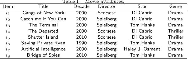
Table I. Movie attributes.
Item Title Decade Director Star Genre
i1 Gangs of New York 2000 Scorsese Di Caprio Drama
i2 Catch me If You Can 2000 Spielberg Di Caprio Drama
i3 The Terminal 2000 Spielberg Tom Hanks Drama
i4 The Departed 2000 Scorsese Di Caprio Thriller
i5 Shutter Island 2010 Scorsese Di Caprio Thriller
i6 Saving Private Ryan 1990 Spielberg Tom Hanks Drama
i7 Artificial Intelligence 2000 Spielberg Haley J. Osment Drama
i8 Bridge of Spies 2010 Spielberg Tom Hanks Drama
pairwise preference mining. Following, Section 2.2 describes the related work on pairwise systems and Section 2.3 reviews the literature concerning social recommenders.
2.1 Pairwise Preference Recommender Systems
Let U = {u1, ..., um} be a set of users and I = {i1, ..., in} be a set of items, RU(A1, ..., Ar) be a
relational scheme related to users, andRI(A1, ..., At) be a relational scheme related to items. The
user-item rating matrix in a system withmusers andnitems is represented byR= [ru,i]m×n, where
each entryru,irepresents the rating given by useruon itemi. Table I shows a set of 8 items (movies)
and their attributes. A user-item rating matrix with 7 users and movies ratings in the range [1,5] is illustrated in Table II.
In traditional recommender systems, the recommendation task is based on the predictions of the missing values in the user-item matrix. Pairwise preference recommender systems predicts the prefe-rence between a pair of items with missing values in the user-item matrix. Both types of systems use the predictions to extract a ranking of items and recommend the top-k.
In our work, we focus on thePrefRecframework, a hybrid model-based approach to design pairwise
preference recommender systems. EssentiallyPrefRecworks in two phases: (A) construction of the
recommendation models, and (B) recommendation.
A) Construction of the recommendation models. The main activities of this phase are Preferences Clustering, Consensus Calculus and Preference Mining.
Preferences Clustering: First,PrefRecclusters users according to their preferences. This
pro-cess applies a distance function and a clustering algorithm C over the rows of the user-item rating matrix. A preference vector of useruxis defined asθux =Rux, whereRux is a row of matrixR. The output of the clustering algorithm is a set of clustersC, where each clusterCshas a set of users with
the most similar preference vectors.
Consensus Calculus: For each cluster Cs, a consensus operatorAis applied to compute ˆθs, the
consensual preference vector of Cs. ˆθs,j is the average rating for item j in clusterCs. Please note
that the ˆθs,j element is computed if and only if more than half of the users in Cs rated the item.
Otherwise, this position will be empty.
An example of clustering and consensus calculus can be seen in Table III. The users from Table II were clustered in two groups according to their preference vectors, and a consensual preference vector for each cluster was computed using the group average rating per item.
Table II. User-item rating matrix. i1 i2 i3 i4 i5 i6 i7 i8
Ted 5 2 - 1 - 2 1
-Zoe 5 2 4 1 5 1 - 3
Fred 4 - 5 - 5 - 1
-Mary 2 5 3 5 - - - 5
Rose 1 - 2 - 2 - - 4
Paul - - 3 4 1 - - 5
John 2 - - 5 2 - -
-Table III. Clusters of users with consensual preferences. i1 i2 i3 i4 i5 i6 i7 i8
Ted 5 2 - 1 - 2 1
-Zoe 5 2 4 1 5 1 - 3
Fred 4 - 5 - 5 - 1
-ˆ
θ1 4.7 2.0 4.5 1.0 5.0 1.5 1.0 *
Mary 2 5 3 5 - - - 5
Rose 1 - 2 - 2 - - 4
Paul - - 3 4 1 - - 5
John 2 - - 5 2 - -
-ˆ
θ2 1.3 * 2.7 4.7 1.7 * * 4.7
Preferences Mining: Having the consensual preference vector from each cluster, the system
could establish the preference relation between pairs of items. Formally, a preference relation is a strict partial order overI, that is, a binary relation P ref ⊆I×I transitive and not reflexive. We denote byi1> i2 the fact thati1is preferred toi2. According to the previous example, a preference
relation over consensual preference vectorθ1 is presented in Table IV.
A preference miner P builds a recommendation model for each group using item’s features. The set of recommendation models isM ={M0 = (ˆθ1, P1), . . . , MK = (ˆθk, PK)}, whereK is the number
of clusters, ˆθsis the consensual preference vector, andPsis the preference model extracted from ˆθs,
for 1≤s≤K.
In this scenario, a recommendation model is a contextual preference model. Thus, each modelPs
inM is designed as aBayesian Preference Network (BPN) over a relational schemaRI(A1, ..., At). A
BPN is a pair (G, ϕ) whereGis a directed acyclic graph in which each node is an attribute, and edges represent attribute dependency;ϕis a mapping that associates to each node ofGa set of conditional probabilitiesP[E2|E1] of the form of probability’s rules: A1=a1∧. . .∧Av=av→B=b1> B =b2
whereA1, . . . , AvandBare item attributes. The left side of the rule (condition eventE1in conditional
probability) is called the context and the right side (condition event E2 in conditional probability)
is the preference on the values of the attribute B. This rule reads: if the values of the attributes
A1, . . . , Av are respectivelya1, . . . , av then for the attributeB the valueb1 is preferred to b2 . Please
note that the preferences onBdepend on the values of the context attributes. A contextual preference model is able to compare items: given two itemsi1 andi2, the model can predict which is preferred.
The constructing of a BPN comprehends in: (1) the construction of a network structure represented by the graphGand (2) the computation of a set of parametersϕrepresenting the conditional proba-bilities of the model. The preference miner used in this work,CPrefMiner[de Amo et al. 2013], uses
a genetic algorithm in the first phase to discover dependencies among attributes and then, compute conditional probabilities using the Maximum Likelihood Principle [Nielsen and Jensen 2009].
Example Overview. Considering the relational schema of movie attributes in Table I and the user-item rating matrix in Table II: PrefRec cluster users, extract preference consensual vector, from ˆθ1
(Table III), and builds the pairwise preference relation (Table IV). Then,CPrefMinercan build the BPN depicted in Figure 1. P N et1represents the contextual preference model that is used to compare
the set of pairs of items and make the predictions.
B) Recommendation. In its second phase,PrefRecaims at using a recommendation modelMsto
recommend items for anew user. It is executed online, in contrast to the first phase which is offline. The recommendation process is executed according to the following steps:
(1) Given a target useruxand a (small) set of ratings provided by ux over some items ofI, the first
task consists in obtaining the consensual preference vector ˆθs more similar to ux’s preferences.
We compute the similarity betweenθu(theux’s preference vector) and each consensual preference
Table IV. C1 pairwise
preference relation (i1> i2)
(i1> i3)
(i3> i6)
(i5> i6)
(i2> i6)
(i5> i3)
(i2> i4)
(i6> i7) Fig. 1. Bayesian Preference NetworkPNet1overC1preferences.
(2) Consider the preference modelPs corresponding to ˆθs. Psis used to infer the preference between
pairs of items inI which have not been rated by the userux in the past.
(3) From the set of pairs of items (ij, ik) indicating that useruxprefers itemijto itemik, a ranking can
be built by applying a ranking algorithm adapted from the algorithmOrder By Preferences
[Cohen et al. 1999]. Thus, the output is a ranking (i1, i2, . . . , in) where an itemij is preferred or
indifferent to an item ik, forj < kandj, k∈ {1, ..., n}.
Example: To illustrate how a preference model can be used in a recommendation phase, suppose that the preference vectorθuof anew userux is most similar to the consensual preference vector of
groupC1, ˆθ1. Let us consider the BPNPNet1built over ˆθ1and depicted in Figure 1. This BPN allows
to infer a preference ordering on items over relational schemaRI(Decade, Director, Star, Genre) of data movie setting. For example, according to this ordering, itemi5 = (2010, Scorsese, Di Caprio,
Thriller) is preferred than itemi8 = (2010, Spielberg, Tom Hanks, Drama). To conclude that, we
execute the following steps:
(1) Let ∆ :I×I→ {Ai, ..., Al}be the set of attributes for which two items differ. In this example,
∆(i5, i8) ={Director, Star, Genre}.
(2) Let min(∆(i5, i8)) ⊆ ∆(i5, i8) such that the attributes in min(∆(i5, i8)) have no ancestors in
∆(i5, i8). According to thePNet1structure, directed edge linkingGenreandStar implies remove
Star, therefore, in this example, min(∆(i5, i8)) ={Director, Genre}. To havei5 preferred rather
thani8 is necessary and sufficient thati5[Director]> i8[Director] andi5[Genre]> i8[Genre].
(3) Computing the probabilities:p1=probability thati5> i8=P[Scorsese> Spielberg]∗P[T hriller >
Drama] = 0.8∗0.66 = 0.53;p3=probability that i5> i8=P[Spielberg >Scorsese]∗P[Drama >
T hriller] = 0.2∗0.33 = 0.06;p2=probability thati8andi5are incomparable= 1−(p1+p3) = 0.41.
To compare i5 and i8 we focus only on p1 and p3 and select the highest one. In this example,
p1> p3 so that we infer thati5is preferred toi8. Ifp1=p3 was true, we would conclude thati5and
i8are incomparable.
2.2 Studies on Pairwise Preference Recommendation
Balakrishnan and Chopra [2012] have proposed an adaptive scheme in which users are explicitly asked for their relative preference between a pair of items. Though it may give an accurate measure of a user’s preference, explicitly asking users for their preference may not be feasible for large numbers of users or items, or desirable as a design strategy in certain cases. Park and Chu [2009] proposed a pairwise preference regression model to deal with the user cold-start problem. We corroborate with their idea. They argue that ranking of pairwise users preferences minimize the distance between real rank of items and then could lead to better recommendation for a new user.
We build on previous work [de Amo and Oliveira 2014] by adapting a pairwise preference recommender to leverage a graph of information, social network.
2.3 Studies on Social Recommender Systems
This research field especially started because social media content and recommender systems can mu-tually benefit from one another. Many social-enhanced recommendation algorithms are proposed to improve recommendation quality of traditional approaches [Krohn-Grimberghe et al. 2012] [Alexan-dridis et al. 2013] [Canamares and Castells 2014]. In terms of using user’s social relationships to en-hance recommender systems effectiveness, there are some common themes betweenSocial PrefRec and the works of Ma et al. [2008] [2011] [2011]. They developed two approaches called SoRec and SoReg. The former is based on probabilistic matrix factorization to better deal with data sparsity and accuracy problems. The latter also relies on a matrix factorization framework, but incorporates social constraints into its built models.
Furthermore, TrustMF is an adaption of matrix factorization technique to map users in terms of their trust relationship, aiming to reflect reciprocal users’ influence on their own opinions [Yang et al. 2013]. SocialMF also explores the concept of trusting among users, but in the sense of propagation into the model [Jamali and Ester 2010]. In comparison, the goal of Social PrefRec is to exploit
social networks in pairwise preference fashion. Although we also employ both users’ social network information and rating records, we do it in a different way. Instead of embedding social information in recommendation models, we built a loosely coupled approach based on clustering techniques to choose a suitable model for a given user.
3. SOCIAL PREFREC
Social PrefRecproposes a new approach to address the new user problem through social information.
It is a PrefRec framework extension, incorporating social information at recommendation phase. There were no modification on how models are built, but at recommendation phase we propose an alternative based on social information to recommend items for new users.
In a simple way, a recommendation for new users using social information could recommend items well rated by his direct friends. Another option is to leverage the connection weight among friends to provide better recommendations. The challenge here is to determine how much influence or similarities exist among user’s relationship. Connect weight among users can be computed through similarities on profiles (profession, age bracket, location, etc.), interaction between users (messaging, photos, etc.) and degree of influence.
To support this feature, we extendedPrefRecand devise Social PrefRec. Figure 2(a) presents
its new structure. To better understand it, let us consider the set of usersU and the set of items I
aforementioned in Section 2. The weight functionw:U×I →Rcomputes auser preference degree for an item and can be represented by a ratingru,i from a user-item rating matrix R. To represent
a social network, let G= (V, E) be a social graph, andux and uy vertices of this graph (users of a
social network). A set of friends (neighbors) of a vertexux is F(ux) ={uy|uy ∈V ∧(ux, uy)∈E}
and a functionl:F →Rdefinesconnection weight betweenux anduy in [0,1].
(a) (b)
Fig. 2. (a)Social PrefRecstructure and (b) Social network example.
3.1 Social PrefRecFramework
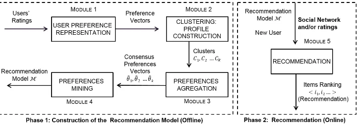
The general architecture ofSocial PrefRec, the interactions among the five modules, as well as their
respective input and output are presented in Figure 3. Modules from 1 to 4 are fromPrefRec, but in module 5 (Recommendation),Social PrefRec, unlike its predecessor, chooses proper recommendation model using one social metric according to following steps.
(1) Given a target user ux and a social metric, we will select ux’s friends F(ux) and the related
connection weight, previously computed as described in Section 3.2, between ux and each uy ∈
F(ux).
(2) Using one of the selection model methods (see Section 3.2), we will select the preference model
Pscorresponding to the clusterCswith more similar friends.
(3) Psis used to infer the preference between pairs of items inI.
(4) From the set of pairs of items (ij, ik) indicating that userux prefers itemij to itemik, a ranking
can be built as mentioned inPrefRecapproach.
Note that using this strategy, it is possible to recommend to a given user without taking into account any previous ratings, but relying on the user’s relations in the cluster set.
3.2 Computation of connection weights and recommendation model selection
Given the social graphGfor a target useruxand for eachuy∈F(ux), we compute user’s connection
weight according the following metrics:
—Friendship: in this metric, connection weight is measured by l(ux, uy) = 1, where 1(·) is the
characteristic function (1 if argument is true, 0 otherwise).
—Interaction level: computed as a(ux,uy) b
a(ux) , wherea(ux, uy) is the number of times that useruyappears atux’s time-line, andba(ux) is the number of all occurrences of usersuy atux’s time-line.
—Mutual friends: Represents the fraction of common friends or Jaccard similarity usingl(ux, uy) = F(ux)∩F(uy)
F(ux)∪F(uy).
—Similarity score: Given by demographic similarity betweenuxanduyaccording to functionl(ux, uy) =
sims(ux, uy). We compute this value by the average of individual similarity in each demographic
attribute (Age bracket, Sex, Religion, etc), using the binary functionsimilarity(ux, uy, Ai), wich
returns 1 if attributeAi is similar foruxanduy, 0 otherwise.
—Centrality: Calculated by average of closeness, betweenness and eigenvector centrality measures withl(ux, uy) =centrality(uy).
Social PrefRecallows the definition of any strategy to find a recommendation model. To do so,
Module 5 provides a function to select a recommendation model. Letselect:U →M be a function that selects the proper recommendation model from M for a target userux. In this work, Social
PrefRecuses two strategies for recommendation model selection based on connection weights:
mini-mum threshold and average connection weight. Each strategy has a different type of implementation for functionselect, as explained in the following definitions:
—Minimum threshold: Letε∈[0,1] be a minimum threshold for connection weight. The minimum threshold strategy selects the preference modelPs(associated with modelMs∈M) which has more
users who have a connection weight with the target userux equal or above a minimum threshold
according to Eq. (1).
select(ux) = arg max
Ms∈M
|{uy∈F(ux)∧l(ux, uy)≥ε}| (1)
—Average: The average strategy selects the preference model Ps with users who have the highest
average connection weight with the target useruxaccording to Eq.(2).
select(ux) = arg max
Ms∈M 1
|F(ux)|
X
(ux,uy)∈F(ux)
l(ux, uy) (2)
4. EXPERIMENTAL SETTING
4.1 Datasets
Table V summarizes our datasets. Recall that sparsity is the percent of empty ratings in user-item rating matrix and links are the number of users connections in the dataset. The particularities of each dataset is described next:
Facebook Dataset. We surveyed this dataset through a Facebook web application we developed for this purpose. With volunteers permission, we crawled relationship status, age bracket, gender, born-in, lives-in, religion, study-in, last 25 posts in user’s time-line, posts shared and posts’ likes, and movies rated before on the Facebook platform. In addition, we asked each volunteer to rate 169 Oscar nominated movies on a 1 to 5 stars scale. We got data from 720 users and 1,454 movies, resulting in 56,903 ratings.
Table V. Dataset features.
Dataset Users Items Ratings Sparsity Rates/User Links Links/User
(%) (Average) (Average)
F B50 361 169 44.925 26.36 124.44 2,926 8.6
F B100 230 169 35,459 8.77 154.16 1,330 6.4
F lixster175K 357 625 175,523 26.36 491 706 2.8
F lixster811K 1,323 1,175 811,726 47.78 613.54 6,526 5.34
overall system performance under datasets with different sparsity and social information levels. The movie’s attributes are: genres, directors, actors, year, languages and countries. In FB50 and FB100, we compute user similarity metric using the attributes: relationship status, age bracket, gender, born-in, lives-born-in, religion and study-in. We also compute the interaction level considering the last 25 posts in the user time-line, posts shared and likes.
Flixster Dataset. Jamali and Ester [2010] published this dataset. However, movie information was restricted to its title, then we improved it by adding genres, directors, actors, year, languages and countries information retrieved from IMDB.com public data. We also use two datasets from Flixster with different sparsity level, Flixster 175K and Flixster 811K. Flixster social information includes friend’s relationships, mutual friends, friends centrality and users similarities. Similarity between users is computed only through three attributes: gender, age bracket and location. Interaction information is not available on Flixster dataset.
4.2 Comparison Methods
In our experiments we compareSocial PrefRecwithPrefRecand three social matrix factorization based recommender systems. The idea is to evaluateSocial PrefRecrecommendations compared to
PrefRec. Note that the former chooses the prediction model using only social information whereas the
latter needs user’s first ratings to choose a model. Further, the comparison with matrix factorization methods is used to evaluate Social PrefRec compared to other social approaches, which handle cold-start users.
Social matrix factorization methods combine social information with rating data. They are distinct from Social PrefRec that uses social information only to choose a consensual prediction model
between preference clusters. In addition, our method has its recommendation model based on pairwise preferences. The three social matrix factorization methods do not make use of any clustering technique. We take these systems as comparison methods because they achieve high accuracy levels for cold-start user as reported by the authors. The social matrix factorization particularities are reported next:
SoRec [Ma et al. 2008]: it is based on latent factors of items, users, and social network relationship. The influence of one neighbor on the prediction of a rating increases if he is trusted by a lot of users while it decreases if the target user has many connections.
SocialMF [Jamali and Ester 2010]: applies a trust propagation mechanism. More distant users have less influence (weight) in rating prediction than the trust direct contacts.
TrustMF [Yang et al. 2013]: represents the influence of connections to target user preferences in two ways: truster and trustee. This approach provides recommendations to users that usually show influence on others and those who are typically influenced by others.
4.3 Experimental Protocol
PrefRecandSocial PrefRecbuild clusters (K-Means clustering) of similar users using the training
set. For each clusterCs the systems associate a recommendation model Ms. Then, to recommend
items for a given userux, it is necessary to select the most similar model (cluster) that fits ux. This
process is done during the test phase. However, those approaches take different directions. Since
PrefRecis not able to deal with social information, it relies on previous ratings of ux to select its
best recommendation model. In contrast, asSocial PrefRecrequires social information to accomplish
this task. We employ the leave-one-out protocol [Sammut and Webb 2010] to better validate our tests and simulate a realistic cold-start scenario. Thus, for each test iteration, one user is taken for test purpose, and the training set is made of all other users. Each experiment is composed byniterations, wherenis the number of users. Importantly, becausePrefReccannot act in a full cold-start scenario, we givePrefReca few ratings to bootstrap the system.
PrefRecprotocol. ThePrefRecrecommendation model is built offline. For the test phaseyratings
of the current test useruxchosen at random were considered for the choice of the most similar cluster
Cs. Then, computing the similarity between the preference vector of ux, θux, and the consensual preference vector ofCs, ˆθsis a matter of computing theEuclidian distance between these two vectors
weighted by the number of common ratings (z), wheredE(θux,θˆi) =
1 z
q Pz
k=1(θux,ik−θˆi,ik)
2
. Please note that this similarity distance was used for preferences clustering (training) and selection models (test) phases. Finally, for validation purpose, the remaining ratings of the current test userux were
used.
Social PrefRec protocol. Building the recommendation model is done as in PrefRec. However,
during the test phase, we do not take any rating into account. Social PrefRecrequires solely social
information to find the most similar cluster, Cs, according to a given social metric and a model
selection strategy.
Matrix Factorization social approaches protocol. For SoRec [Ma et al. 2008], SocialMF [Jamali and Ester 2010] and TrustMF [Yang et al. 2013] the experimental protocol builds a model Mx for each
userux using friendship preferences information which includes all friend’s item ratings. In contrast
to previous protocols, the recommendation model, Mx, is not a clustered preference model, but a
specific preference model for each user.
Parameter Settings. In our experiments, we use LibRec [Guo et al. 2015] which contains an implementation of SoRec, SocialMF and TrustMF methods with default parameters. We executed Matrix factorization approaches with 10 latent factors and the number of interactions set to 100. We use K-means as the clustering algorithm for PrefRec and Social PrefRec. In addition, we
experimentally test several numbers of clusters. Then we set the optimal number of clusters for each dataset: 7 for FB50, 6 for FB100, 4 for Flixster 175K, and 2 for Flixter 811K. The minimum threshold
has optimal values equal to 0.4 for FB50 and FB100, and 0.1 for Flixster 175K and Flixter 811K. However, we executed experiments related with Q5 and Q6, over FB50 and FB100 with = 0.1 to have more users in the result set to evaluate these two questions.
4.4 Evaluation methods
Regarding our evaluation method, we present results using two metrics: (1) nDCG is a standard ranking quality metric to evaluate the ability of the recommender to rank the list of top-k items [Shani and Gunawardana 2011]. (2) We also compute the standardF1 score, based on precision and
recall, to evaluate the prediction quality of pairwise preferences [de Amo and Oliveira 2014].
In thenDCG equation (3), ru,1 is the rating (according to the ground truth) of the item at the
first ranking position. Accordingly,ru,j is the ground truth rating for the item ranked in positionj.
a target useru,DCG∗(u) is the ground truth and N is the number of users in the result set.
DCG(u) =ru,1+
M X
j=2
ru,j
log2j, N DCG=
1
N
X
u
DCG(u)
DCG∗(u) (3)
Precision and recall were combined usingF1score (Eq. (4)). The precision of a useruis the percentage
of good predictions among all the predictions made for useru. The recall is the percentage of good predictions among the amount of pairs of items in the current iteration. Final precision and recall of the test set are obtained by considering the harmonic mean of average precision and average recall of each user.
F1= 2∗
precision∗recall
precision+recall (4)
Besides those metrics, we further analyze how the user ratings profile length and the number of friends impact the recommendation quality through two other metrics: (1) profile length factor and (2) social degree:
Profile length Factor: Let ¯Rbe an average number of user ratings and anαcoefficient, whereα∈R. Eq. (5) represents the profile length factor calculus. In our experiments (Figure 6(a)) we compute theF1score for different profile length factors to determine the number of ratings necessary to better
select a recommendation model for a given dataset.
P lf actor=α∗R¯ (5)
Social Degree: The social degree is given by the average degree of the social network ( ¯S) and a β
coefficient whereβ∈R. We compute the social degree according to Eq. (6). Using different number of friends to select a recommendation model we evaluate theF1results (Figure 6(b) - 6(f)).
Sd =β∗S¯ (6)
5. RESULTS
In this section, we thoroughly assess the effectiveness of our proposed pairwise preference recommender approach,Social PrefRec. First, we analyze the quality of recommendations on the datasets (Q1). Then, we measure the relevance of recommendations (Q2), focusing on the ranking relevance of
Social PrefReccompared to those provided by three social recommender systems, besides the original PrefRec. Furthermore, we measure the performance for each social metric (Q3) and under different
sparsity levels (Q4). We close this section by analyzing how user’s profile length versus its social degree (Q5) and popular versus unpopular users (Q6) influence the quality of the recommendations.
5.1 How accurately social information help on pairwise preference recommendation? (Q1)
F1scores are represented in Figure 4, for minimum threshold and average connection weight selection
FB100 FB50 Flixter 175K Mu tual Inte racti on Sim ilar ity Frie nd ship Cen tra lity Pre fRec 0.6
0.65 0.7
F1 (a) Mu tual Inte racti on Sim ilar ity Frie nd ship Ce ntra lity Pre fRec 0.6
0.65 0.7
F1
(b)
Fig. 4. F1 scores forSocial PrefRecandPrefRecfor 2 model selection strategies: (a)Minimum threshold and
(b) Average connection weight.
5.2 How relevant are the recommendations made by a social pairwise preference recommender? (Q2)
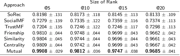
Tables VI, VII, VIII, and IX show the nDCG results for rank size 5, 10, 15, 20, under minimum threshold strategy, Section 3.2, and 0-rating scenario. We apply each approach described in Section 4.3 on each dataset to assess the robustness of each. We observe thatSocial PrefRecobtains better
results for new users compared to the other social recommenders. One of the main reasons for the effective performance of our approach is that it chooses a suitable recommendation model based on a consensual set of friends’ preferences. The other approaches not only consider all friends’ preferences, but SocialMF, for example, also relies on trust propagation mechanism, which incorporates preferences from friends of friends. Thus, we argue that a specific set of friends (neighbors) might be a better source to give more relevant recommendations.
Another main difference is about how each approach deals with item attributes. Matrix factorization profiles both users and items in a user-item rating matrix and through latent factor models project items and users into the same latent space, thus making them comparable.
According to a Kruskal-Wallis test with 95% confidence, Social PrefRec performance is signif-icantly better than social matrix factorization approaches. Mutual Friends is better than others
Social PrefRecmetrics in ndcg@5. For ndcg@10, there is no significant difference between Mutual
Friends, Centrality, Friendship, Similarity and Interaction. The performance with Centrality achieves an equivalent score as Mutual Friends in ndcg@15 results. Finally, the ndcg@20 values show that Mutual Friends, Centrality, Friendship and Similarity are not significantly different.
Table VI. Resulting nDCG@5, @10, @15, and @20 against FB50.
Approach Size of Rank
@5 @10 @15 @20
SoRec 0.8515±.138 0.8412±.123 0.8340±.114 0.8297±.108
SocialMF 0.7469±.183 0.7536±.158 0.7550±.146 0.7576±.139
TrustMF 0.8373±.147 0.8296±.133 0.8259±.122 0.8250±.114
Friendship 0.9870±.035 0.9779±.039 0.9697±.040 0.9612±.042
Similarity 0.9860±.036 0.9770±.040 0.9683±.042 0.9601±.045
Centrality 0.9881±.033 0.9802±.038 0.9721±.039 0.9647±.041
Mutual 0.9934±.025 0.9890±.028 0.9752±.033 0.9665±.038
Table VII. Resulting nDCG@5, @10, @15, and @20 against FB100.
Approach Size of Rank
@5 @10 @15 @20
SoRec 0.8358±.141 0.8251±.124 0.8180±.119 0.8114±.115
SocialMF 0.7124±.193 0.7100±.173 0.7111±.163 0.7166±.155
TrustMF 0.7742±.149 0.7819±.128 0.7835±.120 0.7804±.115
Friendship 0.9852±.036 0.9746±.042 0.9666±.044 0.9582±.046
Similarity 0.9850±.038 0.9746±.042 0.9667±.043 0.9587±.046
Centrality 0.9897±.028 0.9797±.037 0.9706±.041 0.9621±.044
Mutual 0.9933±.023 0.9836±.027 0.9715±.037 0.9636±.042
Interaction 0.9762±.053 0.9762±.060 0.9603±.061 0.9547±.061
Table VIII. Resulting nDCG@5, @10, @15, and @20 against Flixter 175K.
Approach Size of Rank
@5 @10 @15 @20
SoRec 0.8209±.134 0.8236±.120 0.8224±.115 0.8214±.111
SocialMF 0.7715±.138 0.7753±.126 0.7755±.123 0.7751±.120
TrustMF 0.7603±.136 0.7521±.127 0.7494±.123 0.7485±.120
Frienship 0.9840±.039 0.9769±.038 0.9713±.038 0.9671±.039
Similarity 0.9852±.038 0.9779±.037 0.9726±.037 0.9675±.039
Centrality 0.9830±.039 0.9758±.039 0.9704±.038 0.9657±.040
Mutual 0.9916±.023 0.9810±.030 0.9772±.032 0.9766±.030
Table IX. Resulting nDCG@5, @10, @15, and @20 against Flixter 811K.
Approach Size of Rank
@5 @10 @15 @20
SoRec 0.8198±.131 0.8173±.118 0.8145±.113 0.8133±.109
SocialMF 0.7279±.139 0.7335±.122 0.7359±.116 0.7374±.113
TrustMF 0.7204±.135 0.7246±.122 0.7246±.117 0.7298±.113
Frienship 0.9810±.044 0.9748±.044 0.9699±.043 0.9662±.042
Similarity 0.9804±.045 0.9744±.044 0.9696±.044 0.9661±.043
Centrality 0.9809±.044 0.9742±.044 0.9699±.043 0.9667±.042
Mutual 0.9908±.029 0.9812±.036 0.9747±.038 0.9685±.041
5.3 Which social metrics are more important for item recommendation? (Q3)
We perform Kruskal-Wallis test to check statistical significance amongSocial PrefRecmetrics results
andPrefRec, see Figure 4(b). Mutual Friends, Interaction, Similarity are indicated as best perform-ing. Furthermore, Friendship and Centrality results are not significantly different from PrefRec (profile length = 30-ratings) result. Thus, the test shows with 95% confidence, that with the first three metrics we can better recommend in social 0-rating profile scenario than 30-rating profile in a traditional recommender approach. Although the others social metrics achieved the same result as the traditional approach, they need none previous rating from a user.
5.4 How effective isSocial PrefRecto mitigate data sparsity problems? (Q4)
As sparsity is a big challenge faced by recommendation systems, we consider five subsets sampled from FB100. The basic idea is to simulate sparse scenarios where input datasets has many items to be rated with very few/sparse ratings per user. For instance,F B10050 was obtained by eliminating
Table X. FB100 sparse subsets.
F B100 Ratings per user Sparsity (Dataset) (Average) (%)
10 137.9 18.4
20 122.6 27.4
30 107.28 36.6
40 91.8 45.7
50 76.3 54.8
Figure 5 shows thatPrefRecis superior on less sparse datasets. However, the social approaches on
sparser dataset, i.e. F B10050andF B10040, exhibit better recommendations quality, particularly for
Mutual connection weight metric. These results complement previous analyses of Social PrefRec.
5.5 Does social degree affectSocial PrefRecas much as profile length affectsPrefRec? (Q5)
Traditional recommender systems present better performance when they know more user’s preferences. Figure 6(a) shows the prediction performance of PrefRec on two Facebook datasets. We observe
that the recommender predictions get better as the user’s profile gets longer. For instance,PrefRec
achievesF1 equal to 71.18 on FB100 when we use 123 ratings for recommendation model selection
(α= 0.8).
However, withSocial PrefRec, we do not note a correlation between social degree and prediction
performance. Figures 6(b) to 6(f) show the results for different social degrees. The overall picture is the same on all datasets and all social metrics. So, increasing the number of friends to select a recommendation model do not increase theF1 score. This leads us to the next question that further
evaluates all social metrics for higher and lower social degrees.
5.6 Are there major differences between the quality of recommendations considering popular and unpopular users? (Q6)
To investigate the effects of social degree onSocial PrefRec, we begin by recalling the definition of
popular and unpopular users. First, we calculate the average number of friends on the subsetF B50 and F B100. Popular users are those that have more than the average number of friends, whereas unpopular users have only half the average number of friends.
Figure 7 shows the (F1) achieved by Social PrefRecfor each social metric against each subset.
Mu tual
Inte racti
on
Sim ilar
ity
Fri end
ship
Cen tra
lity
Pre fRec 0.55
0.6 0.65 0.7
F1
FB100 F B10010 F B10020 F B10030 F B10040 F B10050
FB100 FB50
0 0.2 0.4 0.6 0.8 1 0.64
0.66 0.68 0.7 0.72 0.74
α F1
(a)
0 0.5 1 1.5 2 0.62
0.64 0.66 0.68
β−F riendship F1
(b)
0 0.5 1 1.5 2 0.62
0.64 0.66 0.68
β−Similarity F1
(c)
0 0.5 1 1.5 2 0.62
0.64 0.66 0.68
β−M utualF riends F1
(d)
0 0.5 1 1.5 2 0.62
0.64 0.66 0.68
β−Centrality F1
(e)
0 0.5 1 1.5 2 0.6
0.62 0.64 0.66 0.68
β−Interaction F1
(f)
Fig. 6. Profile length factor effect (α, see Eq. 5) overF1 measure (PrefRec) in Fig. 6(a). Social degree effect variants
(β, see Eq. 6) overF1 measure in Fig. 6(a) – 6(f).
Note that, the overall performance is similar between each subset. Regarding the major differences between popular and unpopular users, the mutual friends social metric achieves the worst results, which shows the need of larger amounts of friends to better select a recommendation model. On the other hand, the centrality social metric performance shows that it is not affected by the number of friends. Mutu al Intera ctio n Sim ilari ty Frie ndsh ip Centra lity 0.62
0.64 0.66 0.68
F1 FB100-Popular FB100-Unpopular (a) Mutu al Intera ctio n Sim ilari ty Frie ndsh ip Centra lity 0.6
0.62 0.64 0.66
F1
FB50-Popular FB50-Unpopular
(b)
6. CONCLUSION
We have devised and evaluatedSocial PrefRec, an approach whose goal is to help pairwise preferences recommender systems to deal with 0-rating user’s profile. Driven by six research questions, we expand earlier work by analyzing and demonstrating the effectiveness of our proposed social preference learning approach. Our analyses were performed on four real datasets. We also carefully investigate the role of five well-known social metrics in pairwise preference recommendation and proposed a clustering based approach to incorporate social networks into recommender systems. WithSocial PrefRecapproach,
we brought novel ways to extend traditional recommenders.
Finally, although focused on social networks, our work could be extended to tackle other networks (graphs) where we can compute similarity scores between nodes, such as scientific networks or inferred networks [Fel´ıcio et al. 2016]. Another interesting direction for future work is the study of how to choose more influential nodes,e.g. find out the friends who have a stronger influence on a user and apply their preferences to tackle cold-start recommendations.
REFERENCES
Alexandridis, G.,Siolas, G.,and Stafylopatis, A.Improving Social Recommendations by Applying a Personalized Item Clustering Policy. InProceedings of the ACM Conference on Recommender Systems. Hong Kong, China, pp. 1–7, 2013.
Balakrishnan, S. and Chopra, S. Two of a Kind or the Ratings Game? Adaptive Pairwise Preferences and Latent Factor Models.Frontiers of Computer Science6 (2): 197–208, 2012.
Canamares, R. and Castells, P. Exploring Social Network Effects on Popularity Biases in Recommender Systems.
InProceedings of the ACM Conference on Recommender Systems. Foster City, CA, USA, pp. 1–8, 2014.
Chang, S.,Harper, F. M.,and Terveen, L. Using Groups of Items for Preference Elicitation in Recommender Systems. InProceedings of the ACM Conference on Computer Supported Cooperative Work & Social Computing. Vancouver, BC, Canada, pp. 1258–1269, 2015.
Cohen, W. W.,Schapire, R. E., and Singer, Y. Learning to Order Things. Journal of Artificial Intelligence
Research10 (1): 243–270, 1999.
de Amo, S.,Bueno, M. L. P.,Alves, G.,and da Silva, N. F. F. Mining User Contextual Preferences. Journal of
Information and Data Management4 (1): 37–46, 2013.
de Amo, S. and Oliveira, C. G. Towards a Tunable Framework for Recommendation Systems Based on Pairwise Preference Mining Algorithms. In Proceedings of the Canadian Conference on Artificial Intelligence. Montreal, Canada, pp. 282–288, 2014.
de Amo, S. and Ramos, J.Improving Pairwise Preference Mining Algorithms using Preference Degrees. InProceedings
of the Brazilian Symposium on Databases. Curitiba, Brazil, pp. 107–116, 2014.
Fel´ıcio, C. Z.,de Almeida, C. M. M.,Alves, G.,Pereira, F. S. F.,Paix˜ao, K. V. R.,and de Amo, S. Visual Perception Similarities to Improve the Quality of User Cold Start Recommendations. InProceedings of the Canadian
Conference on Artificial Intelligence. Victoria, Canada, pp. 96–101, 2016.
Fel´ıcio, C. Z.,Paix˜ao, K. V. R.,Alves, G.,and de Amo, S. Social PrefRec framework: leveraging Recommender Systems Based on Social Information. In Proceedings of the Symposium on Knowledge Discovery, Mining and
Learning. Petr´opois, RJ, Brazil, pp. 66–73, 2015.
Guo, G.,Zhang, J.,Sun, Z.,and Yorke-Smith, N.LibRec: a Java Library for Recommender Systems. InProceedings
of the Conference on User Modeling, Adaptation, and Personalization. pp. 1–4, 2015.
Jamali, M. and Ester, M. A Matrix Factorization Technique with Trust Propagation for Recommendation in Social Networks. InProceedings of the ACM Conference on Recommender Systems. Barcelona, Spain, pp. 135–142, 2010.
Krohn-Grimberghe, A.,Drumond, L.,Freudenthaler, C.,and Schmidt-Thieme, L.Multi-relational Matrix Fac-torization Using Bayesian Personalized Ranking for Social Network Data. InProceedings of the ACM International
Conference on Web Search and Data Mining. Seattle, Washington, USA, pp. 173–182, 2012.
Ma, H.,Yang, H.,Lyu, M. R.,and King, I.SoRec: Social Recommendation Using Probabilistic Matrix Factorization.
InProceedings of the ACM Conference on Information and Knowledge Management. Napa Valley, CA, USA, pp.
931–940, 2008.
Ma, H.,Zhou, D.,Liu, C.,Lyu, M. R.,and King, I.Recommender Systems with Social Regularization. InProceedings
of the ACM International Conference on Web Search and Data Mining. Hong Kong, China, pp. 287–296, 2011.
Ma, H.,Zhou, T. C.,Lyu, M. R.,and King, I.Improving Recommender Systems by Incorporating Social Contextual
Information.ACM Transactions on Information Systems 29 (2): 9:1–9:23, 2011.
Park, S.-T. and Chu, W.Pairwise Preference Regression for Cold-start Recommendation. InProceedings of the ACM
Conference on Recommender Systems. New York, NY, USA, pp. 21–28, 2009.
Sammut, C. and Webb, G. I. Leave-One-Out Cross-Validation. In Encyclopedia of Machine Learning. Springer,
Boston, MA, USA, pp. 600–601, 2010.
Shani, G. and Gunawardana, A.Evaluating Recommendation Systems. InRecommender Systems Handbook, F. Ricci, L. Rokach, B. Shapira, and P. B. Kantor (Eds.). Springer, Boston, MA, USA, pp. 257–297, 2011.
Sharma, A. and Yan, B. Pairwise Learning in Recommendation: Experiments with Community Recommendation on Linkedin. InProceedings of the ACM Conference on Recommender Systems. Hong Kong, China, pp. 193–200, 2013.
Tang, J., Hu, X.,and Liu, H. Social Recommendation: a Review. Social Network Analysis and Mining 3 (4): 1113–1133, 2013.
Yang, B.,Lei, Y.,Liu, D.,and Liu, J. Social Collaborative Filtering by Trust. InProceedings of the International
Joint Conference on Artificial Intelligence. Beijing, China, pp. 2747–2753, 2013.
Yuan, T.,Cheng, J.,Zhang, X.,Liu, Q.,and Lu, H. How Friends Affect User Behaviors? An Exploration of Social