Equity-Based Insurance Guarantees
by
Nakedi Wilson Leboho
Thesis presented in partial fulfilment of the requirements
for the degree of Master of Science in Mathematics in the
Faculty of Science at Stellenbosch University
Department of Mathematical Sciences, Mathematics Division,
University of Stellenbosch,
Private Bag X1, Matieland 7602, South Africa.
Supervisor: Dr. R. Ghomrasni
Declaration
By submitting this thesis electronically, I declare that the entirety of the work contained therein is my own, original work, that I am the sole author thereof (save to the extent explicitly otherwise stated), that reproduction and pub-lication thereof by Stellenbosch University will not infringe any third party rights and that I have not previously in its entirety or in part submitted it for obtaining any qualification.
Signature: . . . . N.W Leboho
Thursday 19th February, 2015 Date: . . . .
Copyright © 2015 Stellenbosch University All rights reserved.
Abstract
Equity-based insurance guarantees also known as unit-linked annuities are an-nuities with embedded exotic, long-term and path-dependent options which can be categorised into variable and equity indexed annuities, whereby in-vestors participate in the security markets through insurance companies that guarantee them a minimum of their invested premiums. The difference between the financial options and options embedded in equity-based policies is that fi-nancial ones are financed by the option buyers’ premiums, whereas options of the equity-based policies are financed by also continuous fees that follow the premium paid first by the policyholders during the life of the contracts. Other important dissimilarities are that equity-based policies do not give the owner the right to sell the contract, and carry not just security market related risk, but also insurance related risks such as the selection rate, behavioural, mortality, others and the systematic longevity. Thus equity-based annuities are much complicated insurance products to precisely value and hedge. For insurance companies to successfully fulfil their promise of eventually returning at least initially invested amount to the policyholders, they have to be able to measure and manage risks within the equity-based policies. So in this thesis, we do fair pricing of the variable and equity indexed annuities, then discuss management of financial market and insurance risks management.
Uittreksel
Aandeel-gebaseerde versekering waarborg ook bekend as eenheid-gekoppelde annuiteite is eksotiese, langtermyn-en pad-afhanklike opsies wat in veranderlike en gelykheid geindekseer annuiteite, waardeur beleggers neem in die sekuriteit markte deur middel van versekering maatskappye wat waarborg hulle ’n min-imum van geklassifiseer kan word hulle belˆe premies. Die verskil tussen die finansi¨ele opsies en opsies is ingesluit in aandele-gebaseerde beleid is dat die finansi¨ele mense is gefinansier deur die opsie kopers se premies, terwyl opsies van die aandele-gebaseerde beleid word deur ook deurlopende fooie wat volg op die premie wat betaal word eers deur die polishouers gefinansier gedurende die lewe van die kontrakte. Ander belangrike verskille is dat aandele-gebaseerde beleid gee nie die eienaar die reg om die kontrak te verkoop, en dra nie net markverwante risiko sekuriteit, maar ook versekering risiko’s, soos die selek-sie koers, gedrags, sterftes, ander en die sistematiese langslewendheid. So aandeel-gebaseerde annuiteite baie ingewikkeld versekering produkte om pre-sies waarde en heining. Vir versekeringsmaatskappye suksesvol te vervul hul belofte van uiteindelik ten minste aanvanklik belˆe bedrag terug te keer na die polishouers, hulle moet in staat wees om te meet en te bestuur risiko’s binne die aandeel-gebaseerde beleid. So in hierdie tesis, ons doen billike pryse van die veranderlike en gelykheid geïndekseer annuiteite, bespreek dan die bestuur van finansiele markte en versekering risiko’s bestuur.
Acknowledgements
It would not have been possible for me to study towards this degree, so I would like to thank His Grace the most high God for giving me the strength when things seemed likely to deter me the opportunity that African Institute for Mathematical Sciences (AIMS) and Stellenbosch University made available. Thanks to AIMS management for granting me the bursary and made sure I am comfortable with my stay at the institution as I do my studies. To my supervisor Dr. Raouf Ghomrasni who contributed by guiding me and ensuring that I do not just properly construct but also understand my work thoroughly, I say thank you, I learned many things from you that are inspiring and hard work is one of them.
Finally, I thank my family for the support I get that always give me courage to study further.
Dedications
This thesis is dedicated to all my family.
Contents
Declaration i Abstract ii Uittreksel iii Acknowledgements iv Dedications v Contents viList of Figures viii
List of Tables ix
1 Introduction 1
2 Valuation of Variable Annuities 8
2.1 Valuation of the GMDB . . . 10
3 Valuation of GMIB and GMAB 14 3.1 The Pricing GMIB Model . . . 14
3.2 The Pricing of GMAB . . . 19
4 Valuation of GMWB 21 4.1 The Benefit Itself . . . 21
4.2 Model under Policyholder’s Perspective . . . 25
4.3 Model under Insurer’s Perspective . . . 31
4.4 Tree Methodology for Pricing the GMWB . . . 34
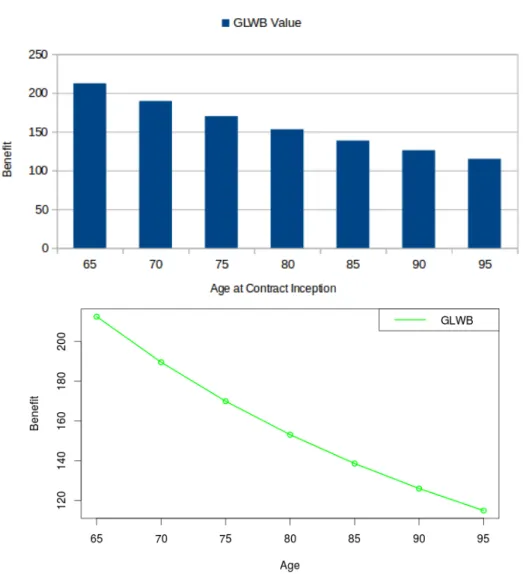
4.5 GMWB for Life Valuation . . . 39
5 Valuation of Equity-Indexed Annuities 43 5.1 Equity Indexed Annuities with Cliquet Option . . . 44
5.2 Equity-indexed annuities with surrender option . . . 48
CONTENTS vii
6 VA/EIA Investment Embedded Risks 52
7 Conclusion 54
Appendices 56
A Modelling Surrender Rates 57
A.1 Analysis of Surrender Rates . . . 57 B Withdrawal rates, Dynamic Solution and Continuation Value
for GMWB 61
B.1 Sustainable Withdrawal Probabilities . . . 61
B.2 Solving for Solution to Dynamic GMWB . . . 63
B.3 GMWB Continuation Value . . . 65
C Valuation Analysis for EIA 66
C.1 Analysis of Equity-Indexed Policies . . . 66
List of Figures
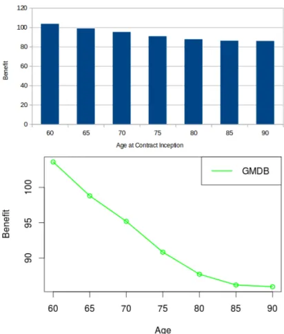
2.1 GMDB Present Values . . . 13
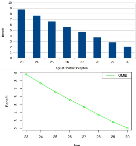
3.1 GMIB Present values . . . 18
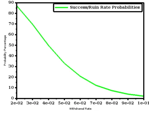
4.1 Success/Ruin Rate Probability Percentages. . . 24
4.2 Base and Account Values under Constant Exhaustion Rate of 4%. 25
4.3 Main idea of incorporated Tree Structures . . . 35
4.4 Withdrawal Period Tree Structure on [0, T∗] . . . 37
4.5 GLWB Present Values . . . 42
A.1 Logit Surrender Rates Response Variables for VA and EIA . . . . 57
A.2 GDP, Inflation and Unemployment data description . . . 58
A.3 Interest Rates data description . . . 58
A.4 Description of non-logit Surrender Rates vs. All Explanatory Vari-ables . . . 59
A.5 VA Logit Function Analysis Output . . . 59
A.6 EIA Logit Function Analysis Output . . . 60
List of Tables
1.1 Insurance Companies in Top Three Markets . . . 3
1.2 Advantages and disadvantages of equity-based annuities. . . 4
4.1 Constant Exhaustion Rate. . . 24
4.2 Fee δ applied on an investment with single premium and varying withdrawals.. . . 28
4.3 Optimal withdrawal values for portion of H whenW = 0. . . 31
4.4 GMWB present values for varying fees and constant interest rate. 34
A.1 Variables Averages and Standard deviations . . . 60
A.2 Correlation for Logit function of VA and EIA with explanatory variables . . . 60
B.1 Withdrawal Success Rate Probabilities (%). . . 62
B.2 Accumulated Period-End Investment Account Values in Dollars ($). 62
C.1 Simple EIA Cliquet Values . . . 67
C.2 Compound EIA Cliquet Values . . . 67
Chapter 1
Introduction
When approaching retirement, people are confronted by a range of financial risks and uncertainties in their lives ahead. A primary concern for them is gaining insubstantial income and the associated problem of outliving their capital. So retirement savings tend to be what people rely on in their older ages. As they enjoy their retirement savings, the question is do these in-vestments provide effectual protections against unfavourable conditions of the market or retirement income risk? As another means of dealing with such a challenge equity-based annuities, also called unit-linked annuities, form part of safer investment and retirement advance arrangements.
Increased life expectancy as well as reduction of the state retirement pensions in several countries led to the rapid growth of equity-based annuities. They have advantageous tax treatment of the proceeds, and at the same time allows participation in the financial/security markets, see Mackenzie (2010). These are specifically retirement designed, long-term financial deals made between investors and investment/insurance companies whereby the companies concur to provide a lump sum payment to some, or payments periodically, starting either immediately or in future time with guaranteed benefits.
Some of the key reasons making equity-based annuities attractive are that: investors finally have a solution to a reduced mortality rate, replacement to pensions, participation in the security market, and alleviation of many invest-ment risks. Even through the recent recession of 2008 there has been a strong demand to these insurance products. These types of investments were intro-duced in the United States in the 1970s, then in the early 1990s insurance companies started including some guarantees in policies of that nature, see Holz et al. (2012). However, the idea of a retirement income came from the Romans with the jurist turned annuity dealer "Gnaeus Domitius Annius Ulpi-anis" who also wrote the first mortality table.
The equity-based types of contracts are divided into two categories, namely,
CHAPTER 1. INTRODUCTION 2
variable annuities (VA) and equity indexed annuities (EIA). Insurance
compa-nies take a certain percentage of the policyholders’ premiums and invest it on their behalf in a portfolio which gives returns that match with a stock index returns, see Marshall (2011). These portfolio returns that the policyholder benefits from are attainable if the market is booming, and when the market condition is unfavourable the policyholder’s investment account does not see a growth but is still protected as an equity-based annuity account.
In VA, the return on the portfolio that the insurance company gets after par-ticipating on behalf of the policyholder is entirely transferred into the policy-holder’s account, whereas in EIA we can have a combination of VA and fixed annuities but the return is capped and floored within a certain interval for the policyholder’s account. These insurance policies come when other means of retirement income becoming increasingly unsustainable.
Because they provide a primal form of lucrative and protected investment, VA and EIA are very popular in the United States and their use now has spread to Japan and many European countries. In 2012, LIMRA Secure
Re-tirement Institute published a report revealing that $159 billion was invested
in variable annuities in US by year end of 2011, see LIMRA (2012). The
Mil-liman Incorporated is an independent international actuarial and consulting
firm that published in August 2011 a survey report on variable annuity devel-opment in Japan. This was led by a principal and senior consultantIno Rikiya, and revealed that about $216.5 billion were invested in variable annuities by March 2011.
In 2010-2011, a financial institution of the European Union called the
Eu-ropean Insurance and Occupational Pensions Authority (EIOPA) conducted a
survey to find out the size of the variable annuities market in Europe and the findings estimated about €188 billion invested in variable annuities, seeEIOPA (2011). A commission created by government congress in the US called
Secu-rities and Exchange Commission that regulates security markets, stated that
about $25 billion was invested in EIA in 2007, and in 2008 the Commission es-timated about $123 billion invested. In South Africa, the available latest data from theFinancial Services Board (FSB) that was analysed by the department of national treasury revealed in 2012 that the annuity market had increased from R8 billion invested in 2003 to R31 billion in 2011, see Treasury (2012). We are yet to see the latest reports estimating total annuity fund invested for 2013-2014 in these countries.
The insurance institutions operating in the world’s three largest annuity mar-kets that offer equity-based policies include among others as displayed in Table
CHAPTER 1. INTRODUCTION 3
US Japan Europe
Jackson National Hartford Life Aegon Prudential Financial Nippon Life Lincoln
Met Life Sumitomo Life Met Life
Nationwide Financial AIG Fuji Life Allianz Transamerica Corporation Nipponkoa Insurance Swiss Life Riversource Annuities Sompo Japan Bayern LB
AIG Tokio Marine AXA Protection
TIAA-CREF Dai-ichi Life Generali Group Ameriprise Financial Manulife Financial Deutsche Bank Hartford Mitsui Mutual Life ING Group
Table 1.1: Insurance Companies in Top Three Markets
Equity-based products mitigate the risk that many retirees will outlast their retirement savings. At inception of the deal, an investor either chooses to make a periodic payment or a lump sum premium to the investment account for later retirement withdrawals. These VA and EIA products have become people’s hope to getting an assured pay-check and something that provides a substitute for the pension. Since they have guarantees, they do not fall under securities in the markets, but insurance policies for some regulatory reasons. The equity-based products are planned out with an intent to protect the in-come against the effect of any unfavourable market condition. Within these equity-based insurance policies tax is included, but it is only taken after with-drawal is made and not as the annuity occurs. What is so advantageous about this is that the amount that would have been deducted for tax annually is compounding and accrues within the annuity. This also suggests that it is lucrative to defer withdrawals rather than making immediate exhaustion. The equity-based products also include a refund feature to a contract. They are successful because they meet most of the requirements and needs of the investors and make easier the decisions about trading them. When entering an annuity contract, there are some options on how long the annuity should last, such as the annuitant’s lifetime, beneficiary’s lifetime, or a pre-specified duration.
When valuing the equity-based products, it is important that people first un-derstand the contract benefits in an insurance policy. In the case where the insurer pays a benefit when a policyholder is still alive, the policyholder bene-fits from a stream of payments or a lump sum where the value GT is received at each maturity date T = t until the expiration date T =T∗. Thus GT is a maturity or a living benefit. However in the case where the policyholder dies first, the benefit as a lump sum is paid to the beneficiary, which is the value
CHAPTER 1. INTRODUCTION 4
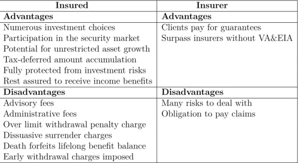
Gtreceived attthtime if the policyholder dies betweent−1 andt, wheret ∈Z+. In Table 1.2 we show the advantages and disadvantages of the equity-based annuities to both the insurance company and policyholder.
Insured Insurer
Advantages Advantages
Numerous investment choices Clients pay for guarantees
Participation in the security market Surpass insurers without VA&EIA Potential for unrestricted asset growth
Tax-deferred amount accumulation Fully protected from investment risks Rest assured to receive income benefits
Disadvantages Disadvantages
Advisory fees Many risks to deal with Administrative fees Obligation to pay claims Over limit withdrawal penalty charge
Dissuasive surrender charges
Death forfeits lifelong benefit balance Early withdrawal charges imposed
Table 1.2: Advantages and disadvantages of equity-based annuities
Surrender and Cliquet Option Features
For insurance companies to meet the needs of customers, equity-based annuity products have had to evolve over time. They are not similar to each other in the way guaranteed amount is decided. Some have features such as
cli-quet/ratchet option, where the guarantee base/balance is reset to equal the
level of the accrued account value during the life of the contract if the annui-tant wants to increase the annual withdrawal percentage.
These features depend on the value of the account at the maturity or death period. The annuitant can make a choice of stepping up payments after a certain period agreed by both parties but with some charges. If for example, the value of the account $45,000 exceeds the guarantee base $34,000, then the guarantee base can be set again to equal the value of the account $45,000. From this information, clearly, it is not wise if not impossible to reset when the base exceeds the account value. For further reading, see Liu (2010). Another feature which is of greater concern to the insurer is the surrender option. This is because the insurer is forced to consider due to unpredictable behaviours of policyholders and circumstances they find themselves in. In this
CHAPTER 1. INTRODUCTION 5
case, due to several personal reasons and unexpected situations, the policy-holder may want to surrender the policy. By surrender we refer to an act of deciding to terminate the contract. On account of the costs the policy provider/insurer experienced when providing the contract, it will cost the pol-icyholder some charges to surrender. The amount of the surrender cash value that the policyholder receives depends on the period the policy is to be sur-rendered.
The earlier the policyholder surrenders the policy the higher the charges, sim-ply because it has never satisfied the insurer’s expectations yet. Also, it can be optimal to surrender the contract if the account valueWtaccrued to exceed the guarantee base Ht. In many companies the surrender value is acquired in the policy if the premiums were paid regularly for at least 3 years. When sur-rendering the contract, all benefits that are associated also terminate. So it is important that the policyholder considers terminating by means of surrender when the policy does not live up to its promises.
Among the factors that trigger the surrenders by policyholders, we have the change in GDP, inflation and unemployment. These can cause the interest rates in the market to drive policyholders to end up surrendering their con-tracts. Usually, when there is an increase in interest rates many people sur-render their contracts and as a result the insurance company’s surplus worsens. When interest rates decrease, the number of people who surrender their con-tracts also falls because surrendering at that period is a lose situation for the policyholder since the account value is low. To model the surrender rates,Kim (2005) suggested that a logit function or what is called a logistic regression model is a suitable model. In this thesis we represent the function by
ln π 1−π =b0+b1·GDP +b2·Inflation +b3·Unemployment +b4·Difference (1.0.1) where the surrender rate is denoted by π, the coefficients that should be esti-mated areb1,b2,b3 andb4, and the factors that represent explanatory variables are as written. The difference of rates represent the interest rates from the security market minus the annuity crediting rate from the insurance company credited to the policyholder’s account. These explanatory variables we men-tioned help to explain any change in the value of the response variable which in our case is the logit function of the surrender rates.
The analysis is as displayed in Section A.1, where the data used for GDP growth, unemployment and inflation are taken from the US Bureau of
La-bor Statistics Department (2014). The surrender rates data is collected from
LIMRA Secure Retirement Institute. The difference of rates is the 30 years Treasury yield rates minus the annuity crediting rates assumed to be 7,5%. The Treasury yield data is from Yahoo.
CHAPTER 1. INTRODUCTION 6
Background Review on Policy Products
In this thesis, the focus of our study is based on pricing and risk management framework of variable annuities and equity indexed annuities, where we will be giving fair prices to these insurance products.
Starting with the Guaranteed Minimum Death Benefit (GMDB), academic re-searchers and market practitioners such asMudavanhu and Zhuo(2002) made a contribution to pricing the death benefit by analysing the benefit with a lapse option as a strategy to increase the account value and expose the insurer to the fee loss. Piscopo(2009) also made analysis of variable annuities and em-bedded option that included the GMDB. In their paper,Marshallet al.(2010) decompose a payoff of the Guaranteed Minimum Income Benefit (GMIB) to analyse its value. Two years later, they again examined the static hedge effec-tiveness, see Marshall et al. (2012).
Kélani and Quittard-Pinon (2014) developed a unified framework of pricing, hedging and assessing the risk existing in variable annuity guarantees including the Guaranteed Minimum Accumulation Benefit (GMAB) in a Lévy market. The recent complex variable annuity product is the Guaranteed Minimum Withdrawal Benefit (GMWB). A breakthrough in the pricing of this benefit was made by Milevsky and Salisbury (2006). In their paper they considered a geometric Brownian motion for investment fund process, and suggested with-drawals are continuous. Their work was partitioned into two strategies of policyholder’s behaviour.
Bauer et al. (2008) generalize a finite mesh discretization technique to model and define a fair price to the GMWB product. Dai et al. (2008) used optimal withdrawal strategy by maximizing the expectation of the discounted value of the cash inflows, and further explored by also applying the penalty charge method suggested to solve singular stochastic models.
Discrete pricing to the product was also part of the framework in Dai et al.
(2008). In their work, some important features such as surrenders and re-sets were included. The most recent popular variable annuity product is the GMWB for life abbreviated as GLWB, short for Guaranteed Lifelong With-drawal Benefit. The product is an extension of GMWB. Holz et al. (2012) priced the product by including different features and taking into account how retiree’s behaviour has an impact to the policy.
In other papers studying the variable annuities such asNgai and Sherris(2011), the strategies in managing mortality risk embedded in variable annuities was investigated. Many other articles published thereafter to improve the frame-work and broaden the strategies in pricing variable annuity products.
CHAPTER 1. INTRODUCTION 7
For equity indexed annuities that will be discussed in this thesis, more in-formation is found in papers such as Hardy (2003), Nielsen and Sandmanne (2002), Bacinello (2003) and many others.
The structure of this thesis is as follows: in Chapter 1, we already gave a necessary introduction that also include a review to the study of equity-based annuities, their advantages, disadvantages and features. In Chapter 2, we be-gin the study of variable annuities by first stating the assumptions for the valuation of all equity-based annuities, then pricing and hedging the first in-troduced VA benefit called the GMDB. In Chapter 3, we do valuation and hedging of the GMIB and GMAB. In Chapter 4, we introduce the most popu-lar variable annuity called the GMWB product, giving a detailed explanation of its features and examples.
With the use of data from Yahoo (2010), we also examine sustainability of withdrawals for a certain chosen exhaustion rate, and eventually formulate pricing model to valuing the GMWB product. We further include its extended form GLWB product in pricing. Lastly, In Chapter 5, we base our study on valuing equity indexed annuities with cliquet and surrender feature.
Chapter 2
Valuation of Variable Annuities
Before getting to the pricing of variable annuities, let us consider the following assumptions underlying the process of pricing the variable annuities.Assume (Ω,F,Q) is a probability space where Ω is a sample space, the fil-tration (Ft)t∈[0,T∗], and Q is the risk neutral probability measure on (Ω,F). The risk neutral probability is known in finance as the probability of future outcomes adjusted for risk, which helps in computing the expectation of asset values. Thus we will make valuations of payment streams under risk neutral measure as the expectation of the discounted values. This assumption also implies that security markets where financial agents are trading is frictionless with no arbitrage opportunities, see Baueret al. (2008).
We assume also under the risk neutral measure Q that the reference equity index value S evolves according to a geometric Brownian motion
dSt= (r−δ)Stdt+σStdBt, S0 = 1, (2.0.1) which has the solution
St= exp[(r−δ− 1 2σ
2)t+σB
t]. (2.0.2) HereB denotes the standard Brownian motion, the fee rate byδ, the risk-free return rate by r, and lastlyσ the volatility of the equity returns. It is in line with the literature of investment account modeling as shown inWindcliffet al.
(2001) and Gerber and Pafumi(2000) to assume that the geometric Brownian motion describes the index dynamics.
Variable annuities can be understood to be a combination of separate/investment accounts with guarantees where the policyholder can choose the asset category he would link to, for example, the NASDAQ, S&P 500, Bond Index or other assets combination. The investment account consists of sub-accounts where all annuitants make premium payments during the accumulation phase.
CHAPTER 2. VALUATION OF VARIABLE ANNUITIES 9
Simulations in the valuation of variable annuities are often the only option since they are complex, exotic, long-term, path dependent and some have no closed form solutions as in standard vanilla options. The other reason the em-bedded options in VA differ from standard vanilla options is that the charges are deducted periodically. Modeling of these charges and fees assumes they are taken as dividends. These insurance benefits are offered mostly by life insurance companies. The valuation of these benefits requires the application of derivatives techniques as they are derivative oriented. To some, annuitants are allowed to access their accounts every time, but surrendering the contract and making withdrawals exceeding yearly guaranteed amount may have harsh penalty charges. As for the guarantees, calculations of the guarantees to be withdrawn are made with reference to their guarantee base. Guarantees in variable annuities are provided even if the account value has gone low. Unlike equity indexed annuities EIA, variable annuities VA have no cap/ceiling on the investment growth.
VA policies have many choices making them even more complex and attractive to investors. There are two main types of VA guaranteed minimum benefits: a death benefit and four living benefits as listed below.
(i). Guaranteed Minimum Death Benefit (GMDB) - Here an assured lump sum is being given to the beneficiary when the policyholder dies. The GMDB and other variable annuity benefits that include a death cover have a stochastic maturity due at the end of the spontaneous exercise period, and also are increasingly put options. The payoff is given by
BD = max(W0egT∗, WT∗), (2.0.3) where W0 is the initial account value at time t = 0, g is the guaranteed rate of growth, and WT∗ is the account value at a random maturity time T∗ when the policyholder dies.
(ii). Guaranteed Minimum Income Benefit (GMIB) - This type of investment is suitable for people who plan to annuitize their contracts. Money saved in the account is annuitized to a stream of guaranteed income for life at a certain point in the future as the maturity after the deferral period. By
annuitization we mean to start a stream of payments from the money that
has been invested and accumulated. If the policyholder dies before the conver-sion period, the beneficiary receives payment by the GMDB whereas after the conversion, the beneficiary is no longer part of the deal. Once annuitization has been triggered it is irreversible, and that means the policyholder has no access to the account value except from receiving a stream of fixed guaranteed income benefits G annually.
CHAPTER 2. VALUATION OF VARIABLE ANNUITIES 10
(iii). Guaranteed Minimum Accumulation Benefit (GMAB) - For this contract, a lump sum guaranteed as the minimum of all deposits is given to the policyholder at a contract maturity date, regardless of the performance of the fund. This accumulation benefit GMAB is also known as the maturity benefit GMMB with a cliquet feature in it, and is a similar contract to the GMDB except the assumption that the policyholder is alive at the maturity date. See Kélani and Quittard-Pinon (2014) and Quittard-Pinon and Randrianarivony (2009) on how the GMMB/GMAB is linked to the GMDB.
(iv). Guaranteed Minimum Withdrawal Benefit (GMWB)- This con-tract is different from GMIB in that it can allow immediate withdrawals, while assuming the retiree is still alive at expiration date. Depending on how much he invested, the policyholder is guaranteed to receive a certain amount each year usually less than 8% of the nest egg invested. Mathematically, we can express it as follows: let G = wH0 = wW0, for w the percentage rate of withdrawal, be the guaranteed annual amount to be withdrawn as long as the guarantee base H is not exhausted at each yearly withdrawal maturity dateT
before the expiration date T∗. Then the final withdrawal at time T∗ is given
by
BW = max(G, WT∗), (2.0.4) which is the greater of the yearly minimum withdrawal and the remaining ac-count value at expiration date.
(v). Guaranteed Life Withdrawal Benefit (GLWB) - The most recent guarantee introduced in 2004 is a hybrid of GMIB and GMWB. The difference is that it is only immediate, and the policyholder can only withdraw a fixed annual amount G for the remaining lifespan without the limit on the total amount that can be withdrawn. This product is usually given to people who wish to start withdrawals from the age of 65.
In the following Section2.1, we start the pricing of variable annuities with the death benefit.
2.1
Valuation of the GMDB
The Guaranteed Minimum Death Benefit (GMDB) product is a withdrawal-deferred annuity contract whereby the policyholder makes a lump sum pay-ment once at contract inception or through periodic paypay-ments to the insurance company as investment premiums. Should the policyholder die, the amount as a lump sum which is the minimum of invested premium, is given to the beneficiary. Main GMDB literature includes that of Mudavanhu and Zhuo
CHAPTER 2. VALUATION OF VARIABLE ANNUITIES 11
(2002), Milevsky (2006), Hardy(2003) and Piscopo (2009).
In this thesis, in a situation where we have only one maturity as in a death benefit GMDB, T = T∗ because the maturity date will also be an expiration
date. We can also think of T∗ conforming to Ta∗ in actuarial literature, as
the remaining future time of life random variable which takes any time t for policyholder aged a, with Fa(t) and fa(t) as its cumulative distribution func-tion and probability density funcfunc-tion respectively. Then the probability that a person aged a dies before reaching the time t is given by
Fa(t) =P(T∗ ≤t)
=tqa = 1−tpa = 1− n−a−t
n−a . (2.1.1)
Heretpais the probability that the policyholder agedawill still be living at age a+t, fort= 0,1,2,· · · , n−a, and n is the terminal age above which aliveness is impossible. Denote again by qa+t the probability that the policyholder of age a+t dies during the course of the following year, then
qa+t = 1−pa+t
= 1
n−a−t. (2.1.2)
Therefore, tpaqa+t = (t|1qa) is the probability that the policyholder of age a, will die between time a+t anda+t+ 1. This survival model is for illustration only and should not be used for any applications. See Dickson et al. (2013) and Hardy (2003) for more on probabilities of survival and death.
In the case of GMDB, we do not have the annual withdrawal guarantee we usually denote by G. Here the personal annuity account value Wt obeys the SDE
dWt= (r−δ)Wtdt+σWtdBt,
where other parameters are as mentioned in equation (2.0.1), see Chu and Kwok (2004) for account and equity values dynamics.
In Hardy (2003), the payoff to the GMDB product at a maturity T∗ is
un-derstood to be
BDT∗ = max(W0egT∗, WT∗), (2.1.3) where g is the guaranteed rate of growth. This payoff can have a valuation that resembles a put option as
CHAPTER 2. VALUATION OF VARIABLE ANNUITIES 12
This suggests the GMDB at a maturityT∗ is the sum of the account value and
an European put option that has a strike priceW0egT∗ and the asset priceWT∗. Let the underlying stock process be St, so WT∗ = ST∗e
−δT∗, and since S t is an index we can set S0 to be whatever we want here. SetW0 =S0. Since we have a stochastic maturity T∗ and the investment account value WT∗ that are independent of each other, the time zero value of the GMDB product can be determined by B0D =Et[EQ[e−rT∗BTD∗|T∗=t]] (2.1.5) =Et[EQ[e−rT∗(max(W 0egT∗ −WT∗,0) +WT∗)|T∗=t]] (2.1.6) =Et[EQ[e−rT∗(max(S 0egT∗−ST∗e −δT∗,0) +S 0e−δT∗)]], (2.1.7) where the expectation inside is taken on WT∗ conditional on the fixed value of
T∗ = t, whereas the expectation outside is taken on all possible values of T∗,
see Carr and Wu (2004). Let the inside expectation with the embedded put option in equation (2.1.7) be denoted as follows
EEP=EQ[e−rT∗(max(S
0egT∗−ST∗e
−δT∗,0) +S
0e−δT∗)]. (2.1.8) By using the Black and Scholes(1973) model to find the embedded put option price, equation (2.1.8) becomes
EEP=W0egT∗e−rT∗Φ(−dB)−W0e−δT∗Φ(−dA) +W0e−δT∗ =W0(e−δT∗Φ(dA) +e(g−r)T∗Φ(−dB)) (2.1.9) where dA = (r−δ−g)T∗+12σ2T∗ σ√T∗ , and dB =dA−σ q T∗. (2.1.10)
Substituting equation (2.1.9) into equation (2.1.7), we have as expressed in general form B0D = Z n−a 0 fa(t)W0 BS(r, g, δ, σ, t) +e−δt dt, (2.1.11) whereBS(r, g, δ, σ, t) represents theBlack and Scholes(1973) put option price. In discrete form, we can express it as
BD0 = n−a X t=1 (tpaqa+t)W0 BS(r, g, δ, σ, t) +e−δt . (2.1.12) Setting the parameters r = 0.05, σ = 0.2, δ = 0.02, g = 0.09, W0 = 100 and n = 100, yields diagrams in Figure2.1 showing the GMDB values’ dependence on the age of the policyholder at contract inception.
CHAPTER 2. VALUATION OF VARIABLE ANNUITIES 13
Chapter 3
Valuation of GMIB and GMAB
The Guaranteed Minimum Income Benefit (GMIB) and the Guaranteed Mini-mum Accumulation Benefit (GMAB) are some of the benefits introduced after the Guaranteed Minimum Death Benefit (GMDB). In this Chapter, we price the two survival benefits starting with the GMIB in Section 3.1, then GMAB in Section 3.2.3.1
The Pricing GMIB Model
The GMIB is a withdrawal deferred insurance policy whereby the policyholder pays a premium payment to the insurer in the form of a lump sum single pre-mium or periodic payments. This will then be invested in the security market to accumulate over time before it can be converted to a stream of annual in-come at retirement time.
Before the conversion of the accumulated amount to an annual income stream by means of annuitization, there is also a choice to withdraw all the accrued amount if the calculation reveals a much higher account value as compared to the guarantee base. This type of benefit is similar to what was known before in the UK as the Guaranteed Annuity Option (GAO), except that the conversion rate applies to the account value or the guarantee base, depending on which one is maximum, yielding a fixed annual income stream, seeHardy(2003) and Kling et al. (2014).
As the income benefit guarantees a lifelong fixed annual payment after annuiti-zation has been made, it implies that the investor is also protected against the longevity risk. During the weak security market conditions, the benefit still serves as a protection during the accumulation phase of the contract. Thus it is a rather challenging contract to hedge with such characteristics.
In this Section, we value the GMIB using the arbitrage free methodology and
CHAPTER 3. VALUATION OF GMIB AND GMAB 15
other model assumptions made in Chapter 2.
Suppose that the policyholder aged a is paid at a retirement date T, either by a lump sum which is equal to the investment value WT linked to the refer-ence equity fund ST, or chose to annuitize for the remaining lifetime and get a stream of guaranteed annual income crHT. Here cr is the conversion rate at which the policyholder converts the guarantee base HT into annuity if the investment fund is equal or lower compared to the base.
As shown in Kling et al. (2014), here the account value WT can be expressed asA0SS0T, whereA0 =W0−δas the amount left after the fee has been deducted by the insurer from the premium. Then the income benefit (GMIB) payoff is expressed by BTI = max(crHTνa+T −WT,0) =ST max cr HT ST νa+T −K,0 , (3.1.1)
where the strike priceK = A0
S0, andνa+T representing the annuity factor which is given by νa+T = n−(a+T) X t=0 tpa+TP(T, T +t). (3.1.2) Here the denotation P(T, T +t) represents the time T zero coupon bond with maturity T +t, and tpa+T is the probability that the person aged a+T still lives at year t.
It is possible in a GMIB contract for the policyholder to annuitize if the in-vestment fund is less than or equal to the guarantee base. So we can assume
HT =ST, which implies that equation (3.1.1) can be written as BTI =ST max n−(a+T) X t=0 P(T, T +t)crtpa+T −K,0 . (3.1.3)
Applying the decomposition suggested by Jamshidian (1989), we may rewrite the GMIB contract payoff that is generated by the zero coupon bond portfolio with Kt strike prices, and tpa+T survival probabilities as weights. Hence we can find fromt = 0,· · · , n−(a+T) the interest rate critical valuer∗ such that
K =
n−(a+T)
X
t=0
P∗(T, T +t)crtpa+T.
From this we define the bond price corresponding with interest rate critical value by Kt which is the new strike price that is artificially introduced as
CHAPTER 3. VALUATION OF GMIB AND GMAB 16
We know that the bond price is a monotonic function of the interest rate. EquivalentlyP(T, T+t) are decreasing functions of interest rater. This implies that ifr∗> r, thenPn−(a+T)
t=0 P(T, T+t)crtpa+T > Kand alsoP(T, T+t)> Kt. Thus max n−(a+T) X t=0 P(T, T+t)crtpa+T −K,0 = n−(a+T) X t=0 crtpa+T max(P(T, T +t)−Kt,0),
and equation (3.1.3) becomes
BTI =ST
n−(a+T)
X
t=0
crtpa+T max(P(T, T +t)−Kt,0). (3.1.4)
The present value under the martingale framework valuation for the GMIB contract of the policyholder aged a at time 0 with maturity T is given by
B0I =EQ " exp − Z T 0 rsds ! TpaBTI # =TpaEQ e −RT 0 rsdsST n−(a+T) X t=0 crtpa+T max(P(T, T +t)−Kt,0) . (3.1.5)
In order to find analytical solutions to equation (3.1.5), it is suitable to measure the payments in stock units instead of values of the money market. So we are to establish a numeraire as the equity price ST and switch from a risk neutral measure Q fixed in the market to equity price measure Qs corresponding to
ST. To comply with Geman et al. (1995) about the change of numeraire, for martingale probability measure Qs equivalent to
Q, we have the density process defined as ψT = dQs dQ |FT (3.1.6) = exp − Z T 0 rsds ! ST S0 . (3.1.7)
This reduces equation (3.1.5) under the new measure Qs to
B0I =TpaS0e−δT n−(a+T) X t=0 crtpa+TEQ s [max(P(T, T +t)−Kt,0)], (3.1.8)
where the expectation in equation (3.1.8) is taken under the equity price mea-sure Qs.
To obtain the expectation of a call option in equation (3.1.8), Vasicek (1977) made the assumption that the term structure of interest rates through the
CHAPTER 3. VALUATION OF GMIB AND GMAB 17
short rate rt evolves as Ornstein-Uhlenbeck process where the bond options are explicitly calculated. The process is expressed as
drt=ϕ(Θ−rt)dt+σdBt (3.1.9) where ϕ, Θ, and σ are positive real constants. The standard solution for the SDE (3.1.9) is given by rt =rse−ϕ(t−s)+ Θ(1−e−ϕ(t−s)) +σ Z t s e−ϕ(t−u)dBu. (3.1.10) We have (rt|Fs)∼N E{rt |Fs}=µr,Var{rt |Fs}=σ2r , where µr=rse−ϕ(t−s)+ Θ(1−e−ϕ(t−s)) σ2r = σ 2 2ϕ(1−e −2ϕ(t−s)) .
A zero coupon bond P(T, T +t) in equation (3.1.8) with expiration T +t at time T is given by P(T, T +t) =eA(T ,T+t)−B(T ,T+t)rT, (3.1.11) where B(T, T+t) = 1 ϕ h 1−e−ϕ((T+t)−T)i= 1 ϕ h 1−e−ϕti A(T, T+t) = 2ϕ 2(ΘB(T, T +t)−Θt) + (t−B(T, T+t))σ2 2ϕ2 − B2(T, T+t)σ2 4ϕ ,
see Björk (2004). For a normally distributed rT, the bond price P(T, T +t) is distributed log-normally with mean M = A(T, T +t)−B(T, T +t)µr and variance V =B2(T, T+t)σ2
r. Then the expectation of a call option payoff via the Black and Scholes(1973) model is given by
EQ s [max(P(T, T +t)−Kt,0)] =FTΦ M −ln(Kt) +V2 V ! −KtΦ M −ln(Kt) V ! =FTΦ (dA)−KtΦ (dB) where FT = eM+12V 2
. Thus from equation (3.1.8), the GMIB present value with a closed form solution to theBlack and Scholes (1973) bond option price is given by B0I =TpaS0e−δT n−(a+T) X t=0 crtpa+T FTΦ (dA)−KtΦ (dB) . (3.1.12) Consider the following parameter values: M = 6.3, V = 0.4, Kt= 90, S0 = 1,
cr = 0.07, δ = 0.001, n = 100, T = 65, and the policyholder’s age at contract inception from a = 23 until a = 30. As depicted in Figure 3.1 we show the GMIB present values for policyholders of different ages.
CHAPTER 3. VALUATION OF GMIB AND GMAB 18
Figure 3.1: GMIB Present values
3.1.1
Hedging GMIB Through Replicating Portfolio
To hedge the GMIB embedded option using the Greeks can be complicated since they are dependent on the interest rate model. If in reality the interest rates and stock prices fluctuations are not reasonably approximated by the model, the hedging via Greeks will not work as explained in Section 3.1 of Marshall (2011) . So the insurer has to, on behalf of the policyholder, make an investment in a portfolio that is replicating where the fee δ = δ∗ is fair if and only if the payoff of the variable annuity with a GMIB option embedded is equal to the total premium expressed asCHAPTER 3. VALUATION OF GMIB AND GMAB 19
A detailed explanation on how financial industries use replicating portfolios for risk management can be found in the research report Milliman (2009).
3.2
The Pricing of GMAB
In this Section, we price the GMAB variable annuity, taking into account a contract with cliquet/reset feature. The GMAB is a survival benefit which needs a fairly long deferred withdrawal period which happens once. If the policyholder dies prior to the expiration date, the contract takes the form of GMDB contract as a lump sum will be given to the beneficiary just as in a death benefit after a waiting period. It is usually called a maturity benefit GMMB with a cliquet option. In our valuation, we assume that the policy-holder will still be alive at expiration date and that the contract has a cliquet feature at any chosen anniversary dates on the interval t ∈(t0, tn].
We apply here as well the assumptions of arbitrage free pricing made in Chap-ter 2. LetWtbi and Wtai be the account value before and after a cliquet option is exercised at an agreed anniversary date ti, then
Wtbi =Wtbi− 1e
m(ti−ti−1) Sti
Sti−1
, (3.2.1)
where m is the rate at which insurer charges the policyholder as also can be seen in Kélani and Quittard-Pinon (2014). The GMAB at timeti is given by
BtA i = max(B A ti−1, W b ti). (3.2.2)
The after reset account value is given by
Wta i =W b ti+ max(B A ti−1 −W b ti,0). (3.2.3)
Under the risk neutral measure, the time zero value for the expiration T∗ of
the GMAB is given by
BpvA =E[e−R t 0rsds×max(BA ti−1 −W b ti,0)]. (3.2.4)
Suppose that the interest rater is constant. Then for the chosen two anniver-sary dates t=t1 and t =t2, we have the present value
BpvA =E[e−rt1max(BAt i−1 −W b t1,0)] +E[e −rt2max(BA ti−1 −W b t2,0)]. (3.2.5) Let us exclude themortality and lapseforces, and use the assumption that the holder is still alive at the expiration date. Also, St0 = Wt0 = BAt0. Then by applying the Black and Scholes (1973) model, we arrive at a closed form solution for the present value of the anniversaries
BpvA =e−rt1BAt0Φ(−dB)−Wt0be −m(t1−t0)Φ(−d A) +e−rt2Bt1AΦ(−dB)−Wt0be −m(t2−t1)Φ(−d A) (3.2.6)
CHAPTER 3. VALUATION OF GMIB AND GMAB 20 where dA = ln( Wt0 BA ti−1 ) + (r+12σ2)(ti−ti−1) σ√ti−ti−1 dB =dA−σ p ti−ti−1. (3.2.7)
For example, suppose the policyholder at contract inception invested a single premium amount of Wt0 = 100, and the other parameters are r= 0.04, m = 0.2, and σ = 0.4. The two reset times are t1 = 3 and t2 = 7, then equation (3.2.6) yields the present value
Chapter 4
Valuation of GMWB
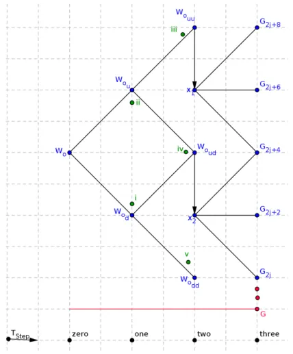
In this Chapter, we begin by explaining the withdrawal benefit and sustain-able withdrawal rates in Section 4.1. We then formulate the model to price the minimum withdrawal and the lifelong withdrawal benefits starting with the static pricing in Subsection 4.2.1under the policyholder’s perspective and the dynamic pricing in Subsection 4.2.2, then in Section 4.3 we employ static pricing under the insurer’s perspective. In Section4.4, we use the tree method-ology by incorporating Cox et al.(1979) binomial, the bino-trinomial, and the stair tree structures by Dai and Lyuu (2010) to find the continuation value of the withdrawal benefit. In Section 4.5 we make valuation of GMWB for life or what is called lifelong benefit GLWB.
4.1
The Benefit Itself
One of the variable annuities people consider purchasing more often for their retirement is the GMWB. Irrespective of whether the account value has de-creased or not, the GMWB product gives the annuitant the possibility of withdrawals that are guaranteed during the life of the deal. In this type of a contract, the annuitant withdraws a certain amount both parties agree upon at contract initiation or can increase withdrawal accepting some penalty. In an instance, when the annuitant dies, the GMWB product will give the ben-eficiary any amount left in the account if the contract is still alive. With the GMWB variable annuity, investors are also enabled to invest in the mar-kets with stocks and bonds but under insurance regulations since they involve guarantees. To impress investors, sometimes the insurer offers that the annu-itant can get bonuses if they do not withdraw within a certain period from the contract initiation. That is, for having a deferred annuity contract with withdrawals at T ≤t ≤ T∗, where T∗ is the expiration date and the maturity
T denotes the time when the policyholder started annual withdrawal after a deferred period t∈[0, T].
CHAPTER 4. VALUATION OF GMWB 22
4.1.1
Sustainable Withdrawal Rates
Before getting deeper into the GMWB study, let us try to understand the calcu-lus of sustainability of withdrawal rates by explicitly explaining and eventually presenting things pictorially.
When a retiree invests in a portfolio and wants to make withdrawals, it is obvious that he may meet the possibility of having his nest egg (total pre-mium invested) exhausted before the expiration date. It should be taken into consideration as an important element to determine withdrawal rates that are sustainable.
One of the questions that may be raised is what withdrawal percentage can be chosen on the retirement savings in order to sustain withdrawal throughout the contract period? This is what investors can ask themselves, since for them to have a greater income in retirement periods, they must choose making higher withdrawal rates from the account. But it has to be noted that the standard of living for such withdrawal rates cannot be sustainable for a longer period. On the other hand, the lower rates of withdrawal would diminish the retirement income but help to reduce the risk of depleting funds in a short period of time. In a popular paper of financial valuation of GMWB written by Milevsky and Salisbury (2006), it is recommended that for half a percentage of asset alloca-tion, the withdrawal rate should not exceed 7% annually as this will shorten the withdrawal period by leading to surrendering of the contract. We will investigate how to wisely choose the exhaustion rate using the calculus of sus-tainable withdrawal rate, where the main idea is to supply investors with an tool to examine different withdrawal rate sustainability for a particular nest egg.
As we proceed below, we make some illustrations on how to estimate the probability of withdrawal success rate and the ruin rate. For example, let us take a retiree who is 45 years old, with 30 years as the median remaining lifetime. The present value of lifetime withdrawals is not normally distributed but distributed closer to a gamma distribution, see Milevsky (2007). Hence, the withdrawal ruin rate probability for a continuous random variableY which takes any withdrawal rate value y with parameters k and φ has a probability density function given by
f(y;k, φ) = 1 Γ(k)φky
k−1e−y
φ k, φ≥0, (4.1.1)
CHAPTER 4. VALUATION OF GMWB 23
The parameters k and φ are given by
k= 2µ+ 4η
σ2+η −1, φ=
σ2+η
2 (4.1.2)
where η is the mortality rate, µ is the expected return rate, and σ represent the volatility of the investment returns. The withdrawal success rate is given by
P(Success Rate) = 1−P(Ruin Rate). (4.1.3) As we continue with our example, let us assume that the nest egg that should finance the stream of annuity withdrawals is $300,000 invested in the NASDAQ Index. Taking the Yahoo (2010) monthly data from (January 1981-December 2010), we can use these values of the parameters k,φ, µandσ. The mortality rate η is given by
η= ln 2
median remaining lifetime, which is η = ln 230 = 0.023 in our case.
As displayed in Table B.1 of Section B.1, we show the calculated withdrawal success rate probabilities for every exhaustion rate mentioned in percentages. In TableB.2, we report the values of the investment portfolio accumulated for every exhaustion rate in every 5 years overlapping end-of-period. Those values are calculated by using the formula
Wt=Wt−1(1 +Rt)−G, (4.1.4) where Wt is the current remaining value of the investment account at the end of the period and Wt−1 is the previous account value at the beginning of the period. The return rateRtof the investment portfolio for periodtis calculated by taking the average of all monthly returns within the specified periods. Looking at the results in Table B.1, we can see the combination of nine rates of exhaustion. For the first five years, based on the withdrawal/exhaustion rate of 2%, the retiree has a withdrawal success rate probability of 87%. It shows the probability percentage of success dropping and eventually declines for the retiree who choose the higher rate of exhaustion over 30 years. Al-though a little more returns can increment the probability of a success rate as displayed on the results, it is also clear that it can never be optimal to increase the rate of withdrawal, for it shortens the retirement income receiving periods and eventually depletes the nest egg before the expiration date. However in equity-based annuities such as GMWB of the variable annuity class, this can never be the case for rational policyholders since they are guaranteed to get
CHAPTER 4. VALUATION OF GMWB 24
the annual fixed withdrawals until the expiration date. However if they are not behaving rationally and withdraw above the limit, then this might result to depletion and eventual surrender. The policyholder will have to pay a penalty charge every time he decides to withdraw any amount above the annual fixed guaranteed amount agreed upon at contract inception. All the results are also represented in Figure4.1showing success/ruin rate probability percentages for each exhaustion rate if chosen over a period of 30 years.
Figure 4.1: Success/Ruin Rate Probability Percentages.
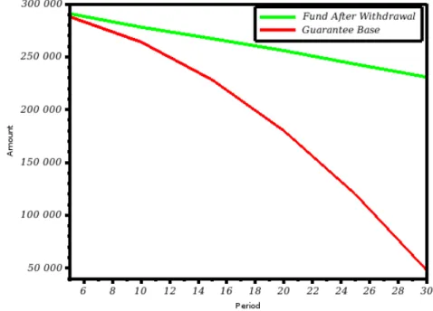
Assuming non-adjusted withdrawals, let us take a constant exhaustion rate of 4% for our example with a nest egg of $300,000. Table 4.1 below reports the results for constant annual withdrawals whereWb,Wa, andHrespectively represent the account value before withdrawal, account value after withdrawal, and the guarantee base.
Years µ(%) Wb Withdrawn Wa H 5 0.95 302849.96 12000 290849.96 288000 10 0.69 302069.96 24000 278069.96 264000 15 1.07 303209.96 36000 267209.96 228000 20 1.3 303899.96 48000 255899.96 180000 25 1.03 303089.96 60000 243089.96 120000 30 0.93 302789.96 72000 230789.96 48000
CHAPTER 4. VALUATION OF GMWB 25
As reported in Table 4.1, our example of 30 years contract deal, shows that for 4% constant exhaustion rate, a retiree’s withdrawal rate is sustain-able. Therefore, in such a case, he can choose to take all remaining amount or extend the contract and step-up/reset since after the 30th year there is still some amount left.
In Figure 4.2 we represent the guarantee base values and the account value under constant exhaustion rate of 4% for our nest egg of $300,000.
Figure 4.2: Base and Account Values under Constant Exhaustion Rate of 4%.
4.2
Model under Policyholder’s Perspective
Before the formulation of the model in Subsection 4.2.1, we first recall all the assumptions made for the pricing of variable annuities in Chapter 2.
4.2.1
Fundamental GMWB Static Pricing
LetWtdenote the GMWB value of the personal annuity account linked to the portfolio at timet, and assume that the initial value of the account is denoted by W0, where the expiration date is T∗ = W0G = w1 with G representing the
guaranteed fixed annual withdrawal amount. If a withdrawal exceeding G is made for some reason, there will be a penalty charge. See Wenger (2012) for more details.
CHAPTER 4. VALUATION OF GMWB 26
The personal account value Wtof the variable annuity with the effects namely the change in guarantee withdrawal base denoted by dHt = −Gdt and the contract fee rate δ, satisfies the SDE
dWt = [(r−δ)Wt−G]dt+σWtdBt, 0≤t≤T∗, Wt >0. (4.2.1) IfWtever hits zero, it stays there. To find the solution of the SDE in equation (4.2.1), we follow techniques by the Itˆo formula. Define the integrating factor by Ft =e(−(r−δ)+ 1 2σ 2)t−σB t. (4.2.2)
For the Itˆo processes F and W, the product rule yields
d(FtWt) =FtdWt+WtdFt+dhF, Wit
=−GFtdt. (4.2.3)
Therefore, the solution to equation (4.2.1) at the expiration time t = T∗ is
given by FT∗WT∗ =F0W0+ Z T∗ 0 −GFsds WT∗ =W0F −1 T∗ −GF −1 T∗ Z T∗ 0 Fsds =W0e(r−δ− 1 2σ 2)T ∗+σBT∗ −Ge(r−δ−12σ 2)T ∗+σBT∗ Z T∗ 0 e−(r−δ−12σ 2)s−σB sds =e(r−δ−12σ 2)T ∗+σBT∗ W 0− W0 T∗ Z T∗ 0 e−(r−δ−12σ 2)s−σB sds ! . (4.2.4) Let XT∗ = e −(r−δ−1 2σ 2)T
∗−σBT∗ which can be perceived as the monetary units that can be bought with a dollar in the annuity account, identical to Euros that can be purchased with a dollar in the foreign exchange market. Then equation (4.2.4) can be written resembling an Asian-Quanto put option as
WT∗ = 1 XT∗ W0− W0 T∗ Z T∗ 0 Xsds ! = W0 XT∗ 1− 1 T∗ Z T∗ 0 Xsds ! . (4.2.5)
An Asian option is one which, unlike European and American ones, has the payoff determined by the average of the underlying asset prices taken over a pre-specified period of time. On the other hand, a Quanto option is one which is expressed in terms of a foreign monetary unit/currency but at an exercise date is converted with a fixed exchange rate to the investor’s home currency,
CHAPTER 4. VALUATION OF GMWB 27
see Datey et al. (2003) to read more on Asian and Quanto options. Hence an Asian-Quanto option is an option of Asian type which is expressed in foreign monetary unit and can be converted at a fixed rate of exchange to investor’s home currency. Moreover, a Quanto option explains that if, for example, an European investor invests in an American stock with NASDAQ index, he is exposed to the rise and fall happening in the NASDAQ and Euro/Dollar ex-change rate.
Let the value of the account’s average be given by ¯ X = 1 T∗ Z T∗ 0 Xsds. (4.2.6)
We know that if Wt reaches zero it stays, and that model equation (4.2.1) holds for Wt >0, ∀ t ≥0. Then under such constraint we can write equation (4.2.5) as
AQPP =FX·max(0,1−X¯). (4.2.7) Here AQPP denotes the Asian-Quanto put option payoff, where FX = XW0
T∗ is the foreign exchange rate, and W0 represents the foreign monetary unit whereas XT∗ is the domestic monetary unit.
For a GMWB policy, the retiree gets the annual withdrawal guarantee and the remaining account value at the expiration date. So the maturity value of the yearly withdrawals or what is also called the term certain annuity is given by Z T∗ 0 Gersds= W0 T∗r (erT∗−1). (4.2.8)
Consequently, the present value of the total cash inflow to a GMWB policy under the policyholder’s perspective is given by the arbitrage free formula
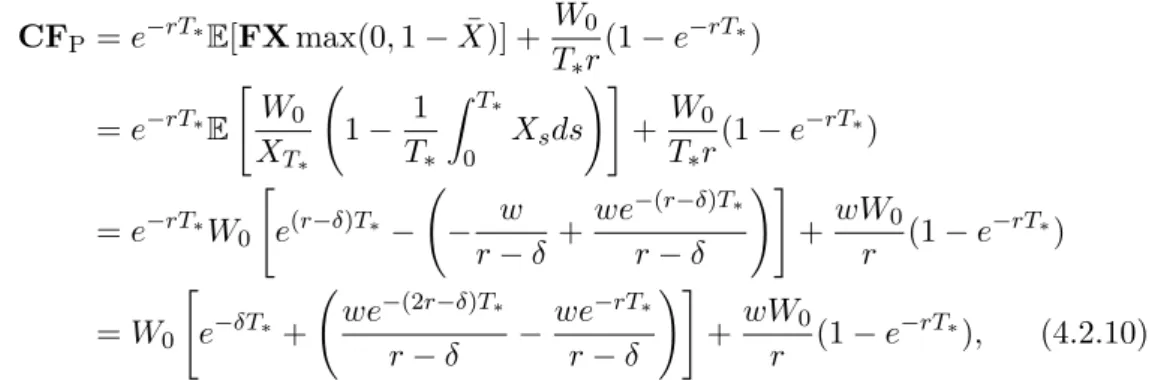
CFP=e −RT∗ 0 rsds E[WT∗] + Z T∗ 0 Gersds =e−rT∗ E[WT∗] + W0 T∗r (1−e−rT∗) =e−rT∗ E[FX·max(0,1−X¯)] + W0 T∗r (1−e−rT∗), (4.2.9) where E[.] is the expectation taken under risk neutral measure. Equation (4.2.9) implies that the cash inflow package of the GMWB under the static valuation is the sum of an Asian put option and a term certain annuity.
CHAPTER 4. VALUATION OF GMWB 28
As an example, let us take $120 to be the value of the account at contract inception denoted by W0, the fixed annual withdrawal amount denoted by G be $8, with the interest rate r of 8%. Then making calculations, the term certain annuity part in equation (4.2.9) is $69.88. That means the option can be purchased with $50.12. Therefore, the GMWB consists of 42% option con-stituent element and 58% of a term certain annuity part.
For ¯X <1 in equation (4.2.7), we have that CFP=e−rT∗E[FXmax(0,1−X¯)] + W0 T∗r(1−e −rT∗) =e−rT∗ E " W0 XT∗ 1− 1 T∗ Z T∗ 0 Xsds !# + W0 T∗r(1−e −rT∗) =e−rT∗W 0 " e(r−δ)T∗− − w r−δ + we−(r−δ)T∗ r−δ !# +wW0 r (1−e −rT∗) =W0 " e−δT∗+ we −(2r−δ)T∗ r−δ − we−rT∗ r−δ !# +wW0 r (1−e −rT∗), (4.2.10)
whereas for ¯X ≥1, the option becomes zero in equation (4.2.7).
Lastly, to fairly value the GMWB product, we equate the total cash inflow
CFP to the policyholder’s investment premium W0 as W0 =e−rT∗E[FX·max(0,1−X¯)] +
W0 T∗r
(1−e−rT∗), (4.2.11) whereby we can find the fair fee as the solution of the expression
e−rT∗ E " FX·max(0,1−X¯) W0 # + 1 T∗r (1−e−rT∗)−1 = 0 . (4.2.12) In Table 4.2 we display the possible fee δ for a single premium of W0 = 100 for interest rate r = 0.07 and different withdrawal rates G.
G T δ 5.5 18.2 0.0451 6.0 16.7 0.053 6.5 13.3 0.061 7.0 14.3 0.069 7.5 13.3 0.079 8.0 12.5 0.088 8.5 11.8 0.096
Table 4.2: Feeδ applied on an investment with single premium and varying with-drawals.
CHAPTER 4. VALUATION OF GMWB 29
4.2.2
GMWB Dynamic Pricing
Under the dynamic pricing, we assume that the policyholder makes with-drawals above, below or sometimes equal to the level G. As also can be seen in Dai et al. (2008), the dynamics of the account valueW obeys
dWt= (r−δ)Wtdt+dHt+σWtdBt, 0≤t ≤T∗, Wt≥0 Ht=H0−
Z t
0
λsds, 0≤λs ≤γ, (4.2.13) where Ht is the guarantee account balance at timet, denotationλs is the rate at which withdrawal is made, and γ is the upper bound. The rest is defined as in equation (4.2.1).
The penalty charge q is deducted for any withdrawal made exceeding the annual fixed withdrawal guarantee value G. On the process of λ exceedingG
(i.e on λ > G), the retiree is certain to get G+ (1−q)(λ−G).
For a cash flow rateg(λ) that the retiree receives from a continuous process of withdrawal, we have that
g(λ) =
(
λ for 0≤λ≤G
G+ (1−q)(λ−G) for λ > G
=λ−qmax(λ−G,0). (4.2.14) The income is received by the retiree throughout the life of the deal, and the account value remaining at an expiration date if it exceeds 0 (i.e if WT∗ ≥0). We assume the retiree is wise and would like to maximise the present value of the cash inflow by choosing withdrawals that are optimal based on the restriction 0 ≤ λ ≤ γ. Then, the GMWB has arbitrage free value at time t
given by ϑ(W, H, t) = max λ Et[e −r(T∗−t)max(0, W T∗) + Z T∗ t e−r(s−t)g(λs)ds], (4.2.15) where Et is the conditional expectation of the expression inside taken under risk neutral measure based on the information at time t.
The pricing formula for the GMWB is found when W = 0, if there is no annuity account participation in the security market any more. Denote by
ϑ0(H, t) the GMWB value when W = 0, which is what we are looking for. To solve equation (4.2.15), we employ the standard procedures that are used when we derive the Hamilton-Jacobi-Bellman equation for problems in stochas-tic control theory, see Dai et al.(2008). Here ϑ evolves according to
∂ϑ
CHAPTER 4. VALUATION OF GMWB 30 with Lϑ= 1 2σ 2W2 ∂2ϑ ∂W2 + (r−δ)W ∂ϑ ∂W −rϑ, (4.2.17) and f(λ) =g(λ)−λ ∂ϑ ∂W −λ ∂ϑ ∂H = λ(1−A) for λ ∈[0, G) qG+λ(1−q−A) for λ ≥G, (4.2.18) where A= ∂W∂ϑ +∂H∂ϑ.
We can obtain the maximum of f(λ) on λ = 0 orG or γ, since it is piecewise linear. Then, the maximum of f(λ) is given by
max λ f(λ) = qG+ (1−q−A)γ for 1−A≥q (1−A)G for 1−A∈(0, q) 0 for 1−A≤0. (4.2.19)
Substituting equation (4.2.19) into equation (4.2.16), we get that
∂ϑ
∂t +Lϑ+γmax(1−q−A,0) + min[max(1−A,0), q]G

![Figure 4.4: Withdrawal Period Tree Structure on [0, T ∗ ]](https://thumb-us.123doks.com/thumbv2/123dok_us/1180103.2658356/47.893.205.684.117.671/figure-withdrawal-period-tree-structure-t.webp)