Heterogeneity and option pricing

Heterogeneity and Option Pricing

Simon Benninga

Tel-Aviv University and University of Groningen [email protected]

Joram Mayshar

Hebrew University, Jerusalem, Israel [email protected] SOM-theme E: Financial markets and institutions

ABSTRACT

An economy with agents having constant yet heterogeneous degrees of relative risk aversion prices assets as though there were a single decreasing relative risk aversion “pricing

representative” agent. The pricing kernel has fat tails and option prices do not conform to the Black-Scholes formula. Implied volatility exhibits a “smile.” Heterogeneous beliefs about distribution parameters also implies non-lognormal pricing kernels with fatter tails and “over-pricing” of out-of-the-money options. Heterogeneity as the source of non-stationary pricing fits Rubinstein’s (1994) interpretation of the “over-pricing” as an indication of “crash-o-phobia”. Rubinstein’s term suggests that those who hold out-of-the-money put options have relatively high risk aversion or relatively high subjective probability assessments of low market outcomes. The essence of this explanation is heterogeneity in investor attitudes towards risks and probability beliefs.

We have benefited from discussions with Antonio Bernardo (our AFA

discussant), Yaacov Bergman, Guenter Franke, Bjarne Astrup Jensen, Shmuel Kandel, Jonathan Paul, and Marti Subrahmanyam, and Zvi Wiener. We also acknowledge the helpful comments of an anonymous referee and René Stultz. Benninga’s research was financed in part by a grant from the Krueger Center for Finance at the Hebrew University.

Heterogeneity and Option Pricing

I. Introduction

In this paper we investigate the pricing of assets in an economy in which there are multiple agents with heterogeneous tastes. The Arrow-Debreu model of general equilibrium under uncertainty does not restrict the heterogeneity of either the

probability beliefs or the preferences of investors. In contrast, in the theories of asset pricing that followed Lucas (1978) there typically exists a representative consumer-investor whose preferences and probability assessments of the economy’s stochastic endowment price all assets. This representative investor is almost always assumed to have time additive preferences with constant relative risk aversion. It is now well-known that the equilibrium framework necessary to derive the Black-Scholes formula for options, given a proportional Brownian diffusion of the underlying payout, requires the existence of such a representative consumer with constant relative risk aversion (see Rubinstein (1976), Breeden and Litzenberger (1978),Brennan (1979), Stapleton and Subrahmanyam (1984), Bick (1987, 1990), and He and Leland (1993) ).

The assumption that all investors have identical homothetic tastes and identical expectations seems particularly unreasonable.1 It is well known that this assumption implies that all investors have identical wealth composition. The empirical evidence seems to contradict this assumption: Mankiw and Zeldes (1991), for example, report that families that do not own any stock account for 62% of disposable income. Another a recent study finds that in 1989 the top one percent of wealth holders held 36.2% of the total non-human worth of United States households and 62.5% of the business assets and corporate stock held by households (Kennickell and Woodburn 1992). In addition, while a representative-agent framework may price all assets, it does not explain why there exists open interest in assets with zero net supply, such as the options, with investors on both sides (short or long) of the market. Some heterogeneity among investors, in either endowments, tastes or

1 _{For a recent criticism of the practice of postulating a single Αrepresentative” agent see} Kirman (1992). A number of recent studies have considered the case of heterogeneity of a different kind: agents who are ex-ante identical end up heterogeneous ex-post, due to the existence of idiosyncratic endowment shocks and due to market imperfections that impede insurance against such shocks (see Mankiw (1986) and the many studies surveyed by Heaton and Lucas (1995) ). We should further note that there are articles within the representative-agent framework where the preferences of the representative representative-agent are not of the constant elasticity type.

opinions seems necessary to explain why such assets will exist at all.2

The formal analysis of the equilibrium underpinnings of the Black-Scholes option pricing formula (for example Bick (1987, 1990) and He and Leland (1993)) retains the presumption of a representative agent. Yet heterogeneity among investors is embedded in most informal discussions of options markets. For example, Cox and Rubinstein (1985, p. 54) give the “use of certain kinds of special knowledge” as one reason for the existence of trade in options. According to such popular views, agents with bullish expectations (perhaps based on “special knowledge”) will be attracted to out-of-the-money calls (written, presumably, by others with more bearish

expectations). On the other hand, out-of-the-money put options are considered to be bought by bearish investors or by investors who are particularly concerned about down-side risk.3

We believe that heterogeneity among agents may also be the key for resolving the empirical non-congruence of the Black-Scholes formula which has attracted a sizeable literature in recent years. In an essentially a-theoretical framework, Rubinstein (1994) and others have attempted to derive a pattern of Arrow-Debreu pricing that is implied by observed option prices (and is inconsistent with the Black-Scholes framework). Franke et. al. (1996) attempt to reconcile this observed pattern within an equilibrium framework where the representative agent displays declining relative risk aversion. In this paper we seek, instead, to examine the case of the pricing of assets and options when all agents have the standard constant-elasticity tastes, but when agents’ tastes, and possibly also their probability assessments, differ.

One may wonder however whether consumer heterogeneity per se could matter. The early formulators of the CAPM were concerned about the effects of the assumption of homogeneity of opinion. As Sharpe (1970) wrote (p. 104): “Even the most casual empiricism suggests that this [homogeneous opinions] is not the case. People often hold passionately to beliefs that are far from universal.” His conclusion, however, was that heterogeneity of opinion is by and large irrelevant since (p. 291) “in a somewhat superficial sense, the equilibrium relationships derived for a world of

2 _{As summarized by Hirshleifer and Riley (1979), with regard to futures trading:}

ΑAmong the possible determinants of speculative activity, John Maynard Keynes and John Hicks . . . have emphasized differential risk aversion . . . . In contrast to these views, Holbrook Working has denied that there is any systematic difference as to risk-tolerance between those conventionally called speculators and hedgers. Working emphasizes, instead, differences of beliefs (optimism or pessimism) as motivating futures trading.”

complete agreement can be said to apply to a world in which there is disagreement, if certain values are considered to be averages.” In a similar vein, Constantinides (1982) established that the asset prices that arise in an economy with heterogeneous agents could be rationalized as if originating from the preferences of a single pricing-representative agent.4

In Mayshar (1977), one of us argued for the pricing relevance of

heterogeneity of opinion, claiming that when some investors are in a corner solution (e.g. all those potential investors in the world who do not hold any particular asset), the sources of the heterogeneity that explain the corner solutions are relevant for the determination of what are the relevant “averages” and thus also for the pricing of assets. Corner solutions, and the identity of actual versus potential investors, are relevant also for the case of heterogeneity in tastes.

In this paper we advance a different argument against the practice of assuming a “representative” investor. As is common in the related literature, we assume that markets are Arrow-Debreu complete, and that all the heterogeneous consumer-investors have “reasonable” time-separable, constant elasticity utility functions with constant time-discount factors, so that no corner solutions exist. We demonstrate that within this framework, when consumers differ with respect to their risk aversion, the induced preferences of Constantinides’s pricing-representative agent are considerably more complicated than those of the actual agents in the economy, and in particular do not belong to the same class of “reasonable” preferences as theirs. In particular, we show that when consumers have different

constant risk aversions, the pricing-representative agent’s preferences exhibit

declining relative risk aversion. The pricing representative consumer’s preferences are thus not of the same class as those of the consumers he “represents.” We demonstrate the significance of this result, and of other sources of investor heterogeneity, for the pricing of options. We show that investor heterogeneity provides a simple and intuitive explanation for the empirical puzzle concerning the non-congruity of the Black-Scholes formula for option pricing with reality. These results cast considerable doubt on the standard practice in the literature of endowing the “representative” agent with “reasonable” (i.e., constant relative risk aversion)

4 _{Constantinides’s representative agent is “representative” only for a given set of endowments} and will not price assets correctly if there is a change in the stochastic endowment. We thus identify the Constantinides representative agent as “pricing-representative.” As Rubinstein (1974) has shown, conditions under which there exists a consumer who is universally representative are extremely restrictive (see also the survey by Shafer and Sonnenschein (1982)).

preferences.

The structure of the paper is as follows: In the following section we set out the equilibrium model, in which all heterogeneous consumers live for two dates. In Section III we characterize the preferences of the “pricing-representative” agent in the model. In Sections IV to VI we illustrate the significance of our findings for the pricing of options in this economy.

II. A two-period Arrow-Debreu economy with heterogeneous agents

We assume a one-good, two-date exchange economy. The aggregate consumption at date 1 (“tomorrow”) is uncertain. We normalize the scale of consumption so that total consumption at date 0 (“today”), Y0, equals to unity. We denote by Ys the

strictly positive total endowment of future consumption in state s, s = 1, ... S. Each agent i is assumed to have a fixed initial fraction of ownership wi of the

economy’s endowment today and in each state of nature tomorrow. We denote i’s initial-period consumption by yi0, and denote by yis the second-period consumption

by agent i in state s. Each of the H agents has time-separable, expected utility preferences that take the form:

(1) U y_i

( )

_i u y_i

( )

_{i i} f u y_{is i}

( )

_is where u y_i

( )

y s S i i = + = − = −

∑

0 1 1 1

β

γ

γ ,

and where fis is agent i’s strictly positive probability assessment of state s, ßi is her

subjective rate of time discount and _γi her constant degree of relative risk aversion.

Each agent is thus characterized by the subjective parameters {ßi, γi, fis } and the

fraction of ownership in the aggregate endowment at dates 0 and 1, wi; we note that

wi is also individual’s i’s fraction of total wealth. We assume ßi> 0, γi > 0, and wi>

0.

We assume the existence of a full initial set of Arrow-Debreu markets, so that in equilibrium there are no potential benefits to trade. Let ps denote the

Arrow-Debreu equilibrium price of contingent consumption in state s. Each agent i selects a consumption program which maximizes Ui(yi ) in (1) given her budget constraint,

(2) y_i p y_{s is} w Y_i p Y_{s s} s S s S 0 0 1 1 + =  +      = =

∑

∑

Let { y ~_i =

{

y_i0,y_i1, ,! y_iS

}

, i = 1, ... , H} be the equilibrium allocation in

the economy. As is well-known, given the particular preferences assumed here, there will be no corner solutions and all ~y_i will be strictly positive. In equilibrium, all

consumers’ marginal rates of substitution equal the state prices: (3)

( )

( )

p f u y u y f y y for all i s s i is i is i i i is is i i = =       −

β

β

γ ' ' , 0 0

The prices ps are determined in a Walrasian equilibrium so as to equate the demand

and supply for all the state-contingent goods.5 (4) y_is Y for all s_S i H = =

∑

₁ ,

Given the particular pattern of tastes in this economy, it is clear that no generality is lost by normalizing Y0 = 1. Let

ωi

=y_i0/Y₀= y_i0 denote agent i’s date

0 share of consumption. The equilibrium prices are, of course, a function of the agents’ characteristics {_βi, γi, fis, wi }, and of market quantities {Ys}. By combining

(3) and (4), we can view psas determined by:

(5)

ω β

γ i i is s s i H _f p Y for all s i       = =

∑

1 1 / ,

This equation determines the equilibrium prices ps as a function of the aggregate

consumption quantities Ys and the agents’ taste parameters. However, the prices in

(5) are dependent on agents’ endogenously-determined shares of initial period consumption {_ωi}, instead of their exogenous initial shares of total wealth {wi}. This

transformation of variables simplifies the presentation below. The equilibrium conditions (3) - (4) and agents’ budget constraints (2) establish a one-to-one relation between agents’ initial distribution of wealth {wi} and the distribution of initial

consumption {ωi}. Given the latter, and given ps as determined by (5), we can

consider the initial wealth fractions as if determined by:

(6) w p f _p p Y i i s i is s s S s s s S i = +    +               = =

∑

∑

ω

β

γ 1 1 1 1 1 /

III. Identifying preferences for a pricing-representative individual

In this section we identify the characteristics of a “pricing-representative” agent in the above economy. We define a “pricing-representative” agent as one whose tastes are such that if all H agents in the economy had tastes identical to his, then the equilibrium state prices in the economy would remain unchanged. As noted in the previous section, it is not possible to find a “representative consumer” who can mimic market prices for any possible set of aggregate endowments {Ys }; we therefore

look for preferences which can mimic the prices in the given economy. We assume that the utility function for the pricing-representative agent takes the separable form: (7) U Y

( )

u Y

( )

f u Y_s

( )

_s s S * ₌ * ₊ * * =

∑

0 0 1

β

The form of the utility function of the pricing-representative agent, (7), assumes time-separability and expected utility maximization, but does not impose the

additional assumption of a constant elasticity temporal utility function assumed in (1) above for each individual.

What we require from this function is that its marginal rates of substitution be equal to the equilibrium state prices ps:

(8)

( )

( )

β

* *' *' , f u Y u Y p for all s s s s 0 0        =

Equation (8) presents a set of conditions from which we can identify properties of the preferences of the pricing-representative agent. Given our normalization Y0 = 1, we define the probability normalized prices q(Y), by the

condition: (9)

( )

( )

( )

q Y u Y u s =        

β

* *' *' 0 1 .

The function q(Y) is sufficient to price all state-contingent commodities, since by (8): (10) q Y

( )

p

f for all s

s s

s

= , .

We now propose to identify properties of the pricing representing agent by making two assumptions:

(i) The set of states of nature is sufficiently dense, so that every level of non-negative future aggregate consumption is possible.

(ii) All agents have homogeneous beliefs that coincide with the objective probabilities, so that fis = fsfor all s and i. In Section IV below we

reconsider the effect of heterogeneous probability assessments. Given these two assumptions it follows by comparing (5) and (8) that we require the pricing function q(Y) to satisfy the implicit condition:

(11)

( )

1/ 1 1, 0 i H i i i for all Y Y q Y γ ω β =   = ≥    

∑

The function q(Y) is implicitly defined by equation (11) for every level of aggregate consumption Y (or in fact for every rate of consumption growth Y/Y0) by the set of

investors’ taste parameters, {ßi, γi } and by the initial consumption shares {ωi },

which, as shown in equation (6) can be taken as a proxy for the initial endowment shares {wi }.

To simplify notation further we make the normalization: u₀*'

( )

1 ₌u*'

( )

1 ₌1_. Setting Y = 1 in condition (9) identifies the time-discount factorβ * _{of the}

pricing-representative agent: (12)

β

*₌q

( )

1 . By (11) it then follows that

(13)

ω β

β

γ i i i H i * /       = =

∑

1 1 1.

It can then easily be established that the representative time-discount factor _β* _is

some average of all agents’ time discount factors ßi, and in particular is between Max i {bi } and Mini {bi }. Conditions (9) and (12) then further identify the temporal utility

function u*_{(Y) as the solution for the differential equation:}

(14)

( ) ( )

( )

u Y q Y q *' = 1

Since equation (14) is assumed to hold as an identity for all non-negative values of Y, we can, by differentiation, define the temporal degree of relative risk aversion of the pricing-representative investor:

(15)

( )

( )

( )

γ

* _Y Yq Y' q Y

= .

Proposition 1: For any Y, _γ*_{(Y) is a harmonic weighted average of individuals’ γ}

i’s. Thus, in particular,_γ*_{(Y) is bounded by Max}

i{γi} from above and by Mini {γi } from

below.

(16) F Y q

( )

y Y q i i i H i , / ≡       = =

∑

0 1 1 1

β

γ _. It follows that: (17)

∂

∂

ω β

γ F Y Y q Y i i i i =       =

∑

2 1 1 / . and (18)

∂

∂

ω

γ

β

α

γ

γ F q Yq q q i i i i i i i i =       =

∑

∑

1 1/ 1 . where (19)

( )

( )

α α

ω

β

γ i i Y _{Y q Y}i i i = ≡       1/ . This means that:

(20) q Y

( )

F Y

( )

F q q Y Y i i i ' / / / / = =

∑

∂ ∂

∂ ∂

α γ

. By its definition in (15), (21)

γ

( )

α γ

* / Y i i i =

∑

1

By equation (3), the weights ai (Y) that were defined in (19), are simply the

second-period consumption shares of agents, when the aggregate endowment is Y. By (11), the αi sum to one. ||

Proposition 1 shows that the risk aversion of the pricing representative consumer is not a simple average of the risk aversions of the individuals in the economy. As we see in the next proposition, this means that for our model, where all the individuals in the economy have constant relative risk aversion, the pricing representative consumer has decreasing relative risk aversion.

Proposition 2: The pricing-representative agent displays decreasing relative risk aversion.

(22)

∂α

∂

α γ

γ

i i i Y = Y −       * 1

Thus, as Y increases, the weight _αi of those investors with relatively low degree of

risk aversion increases. From (21) and (22), (23)

( )

( )

∂ γ

∂

γ

∂ α

∂

α

γ

γ

α

γ

γ α

γ

γ

α

γ

α

γ

* * * * Y Y Y Y i i i i i i i i i i i i i i i i i = − _ _         = −                      =       −        

∑

∑

∑

∑

∑

1 2 2 2 3 ₂ 2

It follows that_∂

γ

*/ Y < 0_∂ if and only if (24)

( )

1 2 2 2

γ

α

γ

α

γ

* =       <

∑

i

∑

i i i i i

Looking at the random variable X that obtains the value 1/_γi with the

probability _αi , we see that the right-hand side above is E(X 2) and the left-hand side is

[E(X)]2_{. Our claim is now established, since the variance of X, EX} 2 _{- (EX)}2_{, has to be}

positive. ||

As the next proposition shows, in states where the aggregate consumption is very high, the “pricing representative” consumer’s RRA looks like the least risk-averse consumer, and vice-versa:

Proposition 3:

(i) If Y _→∞ , then

γ

*_→ Min_i

{ }

γ

_i ; (ii) if Y _→ 0, then

γ

*_→ Max_i

{ }

γ

_i .

Proof: (i) Assume that _γj> Mini {γi } = γk. By (21), it is sufficient to prove that as Y

→∞, _αj→ 0. Suppose to the contrary that αj > ε0 > 0, even as Y →∞. By (21)

then, γ*_{(Y) will be strictly greater than γ}

k, and there has to be ε1 > 0 such that [γ*(Y)/

γk - 1] > ε1. Using (22), dln

( )

α

k / lnd

( )

Y >

ε

1. This differential inequality implies

that as Y _→∞, _αjgrows to infinity, in contradiction to that it is bounded by 1. The

A numerical example

The above propositions demonstrate the complex nature of the preferences of the pricing-representative agent, even in the case where all investor share the same probability assessments. Propositions 2 and 3 imply that the pricing-representative agent displays decreasing relative risk aversion, with _γ*_{(Y) declining from the highest}

rate of relative risk aversion to the lowest as consumption rises. Thus, even though all investors display constant relative risk aversion, it is not the case that the pricing-representative agent will also display constant relative risk aversion, with a

coefficient that is some average of those of the heterogeneous agents in the economy. As we show in the next section, this result has important implications for option pricing.

A numerical example may give some insight into these propositions. Consider a two-date model with 3 possible states at date 1. Aggregate consumption at date 0 is 1, and aggregate date 1 consumption in states 1, 2, and 3 is {0.8, 2, 3}. There are two consumers who have equal initial shares in the consumption at date 0 and in each state of the world at date 1. Each consumer has a utility function with pure time preference _β = 0.99; consumer 1 has RRA _γ1 = 1 and consumer 2 has RRA

γ2 = 7.

An equilibrium solution for the division of aggregate consumption between the two consumers is given in Figure 1 below. Although both consumers consume more in states where the aggregate consumption is greater, the more risk averse consumer 2 has less variability in her consumption than consumer 1. The more risk averse consumer is “more representative” of the equilibrium in state 1 (a low consumption state) and consumer 1 (with low risk aversion) is “more representative” of the equilibrium in state 3, in which there is high aggregate consumption. The result is that the “pricing representative” consumer’s RRA in state 1 (a low consumption state) is higher than the “pricing representative” consumer’s RRA in state 3 (a high consumption state). Thus, although both consumers have constant RRA, the “pricing representative” consumers RRA is decreasing.

Aggregate consumption State price nomenclature

0.80 p1

1 2.00 p2

3.00 p3

Consumer 1 consumption Consumer 2 consumption

0.2938 0.5062

0.4603 1.3693 0.5397 0.6307

2.3200 0.6800

State prices "Pricing representative" consumer's RRA

0.5170 2.0118

0.1109 1.5729

0.0655 1.4723

Figure 1

IV. The pricing of options on aggregate consumption: preliminaries.

In this and the next two sections we apply the results of Section III to the pricing of options in a heterogeneous consumer economy. To simplify the exposition we assume that the economy has only two competitive agents, each endowed with constant relative risk aversion preferences. Each agent is also assumed to believe (correctly) that the probability distribution of aggregate consumption at date 1 is lognormal.

To understand the intuition behind our claim that the pricing of options should be particularly sensitive to heterogeneity among investors, consider the case where the two agents differ in their risk aversion. As shown in the discussion at the end of the previous section, the more risk averse agent seeks to guarantee that the

amplitude of her future consumption will be small, and in particular seeks to protect herself against downside risk. As proved formally in Proposition 3, this agent will thus dominate both the date 1 consumption in states of low aggregate consumption and the pricing of contingent consumption in these states. The less risk averse agent, less concerned with protection against downside risk, will correspondingly dominate in the consumption and the pricing of consumption in high states.

Since an out-of-the-money call option (on total consumption, in this framework) offers the upper tail of the distribution, it follows that its price will be influenced primarily by the attitude towards risk of the less risk averse investor. Symmetrically, the pricing of out-of-the-money put options will be particularly influenced by the attitude towards risk of the more risk averse investor. This intuition thus suggests that the pricing of contingent commodities by any “average” agent, with constant relative risk aversion, will underprice the contingent

consumption in both tails of the distribution, and also tend to underprice out-of-the-money options.

The intuitive discussion above can be alternatively considered as an illustration of Proposition 2, that an economy with heterogeneous agents with constant relative risk aversion will price assets as if it consisted of a single investor with declining relative risk aversion. Another way to present our case is to use Ross’s (1976) idea that options can be considered as completing the market structure, in the absence of trade in state contingent commodities. In this case, if there exists a stock market, and options can be traded for any strike price, both investors in our two-agent economy will hold a long position in the stock. In addition, the less risk averse agent will purchase call options with high strike prices, written by the more risk averse agent. Complementing these transactions, the more risk averse investor will purchase the put options with low strike prices that the less risk averse investor issues. In effect, the two agent will thus be able to obtain a Pareto-efficient

consumption distribution by trading call and put options between themselves. Differential tastes thus provide an intuitive explanation both for the existence of an open interest in options, and for why a constant-relative risk aversion framework is likely to misprice out-of the-money options.

To set the stage for a more formal application of this intuitive logic, we have first to define the relevant assets in this two period economy, and then consider the reference case of asset pricing when the agent are homogeneous. Let p(Y) denote the equilibrium price at date 0 of a unit of date 1 consumption. The interest rate r is determined by the condition that (1+r)-1 _{is the date 0 price of a unit of consumption}

(25)

( )

1 1

( )

0

+r − =∞

∫

p Y dY

We identify the future payout of the “market” in this economy as consisting of the entire date 1 endowment. The date 0 market price S, is thus:

(26) S=∞

∫

Y p Y dY

( )

0

The price of a call and a put option on the market with a strike price of X is therefore: (27) C X

( )

p Y Y X dY

( ) (

)

P X

( )

p Y X Y dY

( ) (

)

X X =∞

∫

− , =

∫

− 0

Denote by

α α

₌

( )

Y consumer 1’s share of aggregate future consumption when the aggregate future consumption is Y and denote by _ω consumer 1’s equilibrium share of date 0 consumption. By (3), the consumption share

α α

₌

( )

Y

and the equilibrium price p = p(Y) are jointly determined by the condition: (28) p= f Y

( )

 ⋅Y f Y

( ) (

)

Y    = − ⋅ −       − −

β

α

ω

β

α

ω

γ γ 1 1 1 2 1 1 2 1 ,

where the function fi (Y) is i’s subjective probability density. Given our assumption

that both agents believe that the distribution of aggregate future consumption is lognormal: (29) f Y

( ) (

f Y

)

[

]

Y Y i i i i i i = = − −      ; ,

µ σ

exp ln

σ

π

σ

µ

1 2 1 2 2 2 . As a reference for the subsequent analysis of the implications of

heterogeneity, we now briefly summarize the well-known results for the case where the two agents are identical, so that the identifying index i can be dropped.

Proposition 4. If aggregate date 1 consumption Y is lognormally distributed and if all investors share identical time-additive preferences with constant relative risk

aversion _γ, then:

(i) The normalized Arrow-Debreu state prices (the “pricing kernel,” or the “risk-neutral probabilities”), (1+r)p(Y), can be considered as the probability density of a lognormal variable with density f(Y; m - _γs2_{, s).}

(30) C X

( )

BS X S r

(

)

SN d

[ ]

X

[

]

rN d = ≡ − + − ; , ,σ

σ

1 , (31) where d= ln /

(

S X

) ( )

+ln1+ +r

σ

2/2

σ

Proof: We do not prove this proposition in detail, since its elements are well known, even if not necessarily in this simple two-period framework (see, Rubinstein (1976), Brennan (1979), or Stapleton and Subrahmanyam (1984) ). For this case the state prices are given by:

(32) p Y

( )

=

β

Y−γ f Y

(

_{; ,}

µ σ

)

=

β

_exp

[

−

γµ γ σ

+ 2 2_/2

]

f Y

(

_;

µ γσ σ

− 2_,

)

where the second equality follows from standard manipulations. Define now the tailed moment-generating-function of the lognormal distribution in (29):

(33) m a x

( )

Y f Ya

(

)

dy

[

a

(

a

)

]

N a x x , ≡ ; , =exp + /  + −ln      ∞

∫

µ σ

µ

σ

µ

σ

σ

2 ₂ 2

where N[z] is the value of the standard normal distribution at z. The two parts of the proposition then follow from applying the definitions in (25)-(27):

(34)

( )

1+r −1=

β

m

(

−

γ

, ,0

)

S =

β

m

(

1−

γ

,0

)

(35) C X

( )

=

β

[

m

(

1−

γ

,X

)

−Xm

(

−

γ

,X

)

]

and then performing the required substitutions. ||

V. The pricing of options with heterogeneous tastes

With the case of homogeneity as a reference point, we now return to the implications of heterogeneity among the two agents in this simple two-period, two-agent

economy. Given our assumptions, the subjective preferences and probability

assessments of each agent will be represented by four parameters: (ßi , γi , µi , σi ) for i

= 1,2, where agent i believes that Y is lognormally distributed with parameters _µiand

σi .

To simplify the presentation, we consider here separately the effect of heterogeneity in only one of these four parameters at a time. Accordingly, we will apply a standard form of notation , where p(Y; _γ1 ,γ2 ) will refer, for example, to the

state price for the case of the given degrees of risk aversion, when this is the only subjective parameter in which the two agents differ.

Since a closed form solution for the state prices p(Y) does not exist for most cases, we will illustrate the implications of several results with a numerical

simulation. In the simulations presented below we use a discrete approximation of the lognormal distribution. For our basic homogeneous case: ß = ß1 = ß2 = 0.9 ,

γ

1=

γ

2=7, µ = µ1 = µ2 = 0.15 , σ = σ1 = σ2 = 0.3. In the heterogeneous risk

aversion case discussed in Section V.b.,

γ

₁=1,

γ

₂=7; for this case we set the initial consumption shares of the agents so that in equilibrium they have equal wealth shares.

V.a. The case of heterogeneity in subjective time discounting

In this case it is assumed that the only subjective parameter in which agents differ is their discount factor ßi. By solving equation (28) for α, it is clear that in this case

each agent’s share of second-period consumption will be a constant, independent of aggregate consumption Y. In fact, this economy will generate state prices p(Y) like the ones in the case of a homogeneous economy, where the representative agent has a discount factor:

(36)

β

*₌

ωβ

₁1/γ _{+ −}

(

1

ω β

)

₂1/γ

As a result, Proposition 4 will apply, and a Black-Scholes formula will price call and put options.

V.b. The case of heterogeneity in risk aversion

This is the main case for which the propositions of Section III should apply. The consumption share of the first agent,

α α

=

( )

Y is here determined by the condition:

(37)

α

( )

(

( )

)

ω

α

ω

γ γ Y Y Y Y       = − −    _ − 1 ₁ − 2 1

There is no analytic solution for the function _α(Y) in this case. However, the following proposition is easily seen to be a corollary of Proposition 3:

Proposition 5. If the two agents differ only in their coefficient of relative risk

aversion and if _γ1 < γ2, then α(Y ), the future consumption share of the less risk averse first agent, will be monotonically increasing in Y, with

( )

( )

lim , lim

Y→0

α

Y =0 Y→∞

α

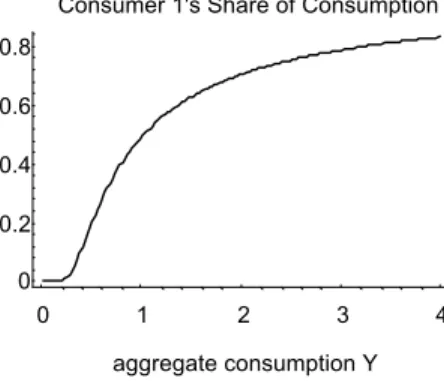
Y =1.

Figure 2 presents the shape of the consumption share function a(Y) for the calibration of the model as described above, where in addition γ1 = 1, γ2 = 7. As

suggested by Proposition 5, and as shown in Figure 2 below, this function is indeed monotonically increasing. 0 1 2 3 4 aggregate consumption Y 0 0.2 0.4 0.6 0.8

Consumer 1's Share of Consumption

Figure 2 As was proved in Proposition 2, as a result of the endogenous non-constant sharing of consumption, the pricing function p(Y) in the case of heterogeneous agents can be interpreted as displaying declining relative risk aversion. It follows from this implication that the pricing kernel (1+r)p(Y) will no longer be lognormally

distributed, as in the homogeneous case, and the Black-Scholes formula will no longer apply. The relevant issue, however, is to identify what specifically will distinguish option pricing in this heterogeneous economy from the option pricing that would apply in a “similar” homogeneous economy. For this purposes we seek to compare the case of the heterogeneous economy with another similar, yet

homogeneous, economy where both agents share some “average” constant coefficient of risk aversion, _γ 0_{. No matter how this average γ} 0 _{is chosen, the following}

proposition applies.

Proposition 6: For any _γ 0_{, such that γ}

1 < γ 0 < γ2, there are two positive values Yhigh

and YRow so that state prices p(Y; γ1, γ2 ) > p(Y; γ 0, γ 0) if either Y > Yhigh or 0 < Y <

Ylow. As a result,

(i) For sufficiently high X, C(X; γ1, γ2 ) > C(X; γ 0, γ 0), (ii) For X sufficiently close to zero, P(X; _γ1, γ2 ) > P(X; γ 0, γ 0).

Proof: From Proposition 5 it follows that since _α(Y) increases monotonically towards 1, when Y approaches infinity,

(38)

(

)

[

( )

]

( )

[ ]

( )

[ ]

( )

(

)

p Y; ,

γ γ

1 2

β α

Y Y γ1f Y

β

Y γ1f Y

β

Y γ f Y p Y;

γ γ

0, 0

0

= − → − > − =

(39)

(

)

[

(

( )

)

]

( )

[ ]

( )

[ ]

( )

(

)

p Y; ,

γ γ

1 2

β

1

α

Y Y γ f Y

β

Y γ f Y

β

Y γ f Y p Y;

γ γ

0, 0

2 21 0

= − − ⇒ − > − =

This proves the first part of the proposition and the implications concerning the pricing of far out-of-the-money put and call options now follow. ||

Since our concern is to examine the impact of heterogeneity on the pricing of options, it is appropriate at this point to illustrate the potential magnitude of the impact of Proposition 6, by use of our calibration example. We compare the option price C(X; _γ1, γ2), where γ1 = 1, γ2 = 7, with the option price C(X; γ 0, γ 0) in a

comparable homogeneous economy where all the parameters are identical and where both investors share the same “average” degree of risk aversion: _γ1 = γ2 = γ 0. It is

not obvious how to define this “average” _γ0_{; at this point we choose to define it so}

that the homogeneous economy will have the correct price for an at-the-money call option.6 _{That is, γ} 0 _{was defined to solve}

C(S(

γ γ

₁, ); , ) = C(S(₂

γ γ

_{1 2}

γ γ

₁, );₂

γ γ

o, )o .

Figure 2 compares the prices of this “average” consumer (for whom we numerically obtained that _γ 0_{= 2.53) with the actual prices in the economy. In the}

graph we show the ratio of these prices p (Y;

γ γ

o, ) / p (Y; ,o

γ γ

_{1 2}).

0 2 4 6 8 10 12 y 0 0.2 0.4 0.6 0.8 1 price ratio

to Actual State Prices

Ratio of Homogeneous State Prices

Figure 3

In accordance with Propositions 3 and 7, the “average” consumer economy generates lower state prices than the actual heterogeneous economy, both for low and for very high levels of aggregate consumption. As a direct result of this key finding, it is not surprising that the homogeneous “average” economy will tend to underprice

out-of-the-money calls.7 This result is depicted in Figure 4 below, which shows the ratio of the actual call option price in the heterogeneous consumer economy C(X; 1, 7) and the Black-Scholes price C(X; _γ 0_{, γ} 0_{), for that homogeneous economy with the}

“average” constant relative risk aversion _γ 0 _{as defined above.}

0 0.25 0.5 0.75 1 1.25 1.5 1.75 x 1 1.01 1.02 1.03 1.04 1.05 1.06 1.07 Call/BS

Call Price in Homogeneous Economy Ratio of Actual Call Price to

Figure 4

The main finding displayed by Figure 4 is that options that are away from the money (whether in or out of the money) are more expensive in this heterogeneous consumer economy than in the Black-Scholes case. The ratio of the call prices depicted in Figure 4 depends, of course, on how we determine the “average” _γ0_.

Were we to choose to normalize on a Black-Scholes option with a different strike price, we would determine a different “average” _γ0_{. We return to this topic in}

Section V.d. below. However, as proved in Proposition 6, the pattern that emerges for out-of-the money options is robust to the selection of the “average” _γ0_.

V.c. Implied volatility: Smiles and heterogeneous consumers

Given the difficulties in estimating the volatility _σ, the Black-Scholes formula is often presented empirically in terms of the stock volatility that is implied by the market pricing of call options with alternative strike prices. Consistency with the Black-Scholes formula should imply a horizontal curve for the implied volatility as a function of the strike price, but the empirical pattern that researchers typically find displays a “smile”.

Given the market interest rate, r(_γ1, γ2 ), and the stock value S(γ1, γ2 ) in the

heterogeneous economy we now solve the Black-Scholes formula in (30) for the implied volatility. That is, for the function BS(.) in (30) and for each X, we

7 _{Franke, Stapleton, and Subrahmanyam (1996) claim that the change in sign exhibit by this} difference is a necessary condition for a volatility “smile.”

determine _σ = _σ(X), such that when _γ1 = 1, γ2 = 7, the following identity holds:

(

) (

)

(

)

(

)

BS X S;

γ γ

1, 2 ,r

γ γ

1, 2 ,

σ

≡C X;

γ γ

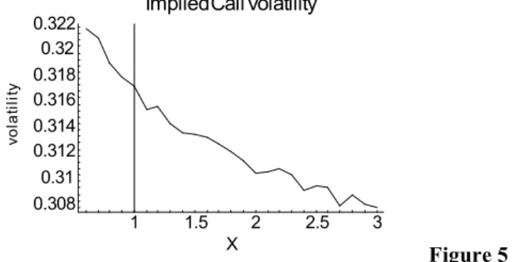
1, 2 .

Figure 5 shows the implied volatility of the call option in our calibrated example (where_σ = 0.3). A smile pattern is evident: The implied volatility for out-of-the money options is lower than that for in-the-money options.8 _{This is the pattern} that is presented (among others) by Rubinstein (1994). As the exercise price of the options gets large, the implied volatility in this simulated example approaches the actual, 30%, volatility of the underlying consumption process from above. This means that for this particular case the implied volatility is everywhere larger than the volatility of the underlying consumption process.9

1 1.5 2 2.5 3 X 0.308 0.31 0.312 0.314 0.316 0.318 0.32 0.322 yti lit al ov ImpliedCallVolatility Figure 5 V.d. Alternative normalizations

In the example of the previous section, we chose a “representative” consumer by determining a risk aversion coefficient γ0 _{so that the price of an at-the-money call in}

the homogeneous consumer economy equals that of an at-the-money call in the heterogeneous consumer economy—C(S(

γ γ

₁, ); , )= C(S(₂

γ γ

_{1 2}

γ γ

₁, );₂

γ γ

0, 0)_.

There are clearly several ways to choose such a normalization:

Case 1: We shall refer to the normalization of the previous section as Case 1:

C(S(

γ γ

₁, ); , )= C(S(₂

γ γ

_{1 2}

γ γ

₁, );₂

γ γ

0, 0)_.

Case 2: Instead of normalizing on an at-the-money call in the heterogeneous

8

The “jagged” pattern in the graph is due to computational rounding problems.

9 _{Franke, Stapleton, and Subrahmanyam (1996) interpret this as meaning that options are “too} expensive.” We have not succeeded in proving that this property will always hold.

economy, we could normalize on an at-the-money call in each economy. That is, we choose _γ 0 _{so that C(S( , ); , )= C(S( , ); , )}

1 2 1 2

γ γ

γ γ

γ γ

0 0

γ γ

0 0 _.

Case 3: In this case we find the “average” relative risk aversion _γ 0 _which

matches the riskless interest rates in both economies:

(

)

(

)

Y 1 2 Y p Y, , dY = p Y, , dY

∫

γ γ

∫

γ γ

0 0

Case 4: In this case we find the “average” relative risk aversion _γ 0 _which

matches the market values in both economies:

(

)

(

)

Y 1 2 Y p Y, , Y dY = p Y, , Y dY

∫

γ γ

∫

γ γ

0 0

The table below summarizes some relevant results for these four cases, and Figure 5 shows the ratios of the actual market price to the homogenous consumer market price (i.e., the Black-Scholes price) for a range of exercise prices.

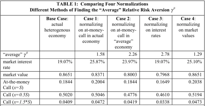
TABLE 1: Comparing Four Normalizations

Different Methods of Finding the “Average” Relative Risk Aversion _γ 0 Base Case: actual heterogenous economy Case 1: normalizing on at-money-call in actual economy Case 2: normalizing on at-money-call in “average” economy Case 3: normalizing on interest rates Case 4: normalizing on market values “average” _γ 0 _{1.58 2.26 2.78 1.29} market interest rate 19.07% 25.87% 23.97% 19.07% 25.10% market value 0.8651 0.8371 0.8003 0.7968 0.8651 At-the-money Call (x=S) 0.1844 0.2004 0.1844 0.1649 0.2038 Call (x=0.5S) 0.5020 0.5046 0.4776 0.4610 0.5194 Call (x=1.5*S) 0.0409 0.0472 0.0419 0.0338 0.0473

Notes: a. The calibrations assume a lognormal aggregate consumption process with _µ = 15%, _σ = 30%. The original economy has two consumers with equal wealth shares and relative risk aversions _γ1

= 1 and _γ2 = 7; each consumer has a pure time discount factor β = 0.9.

b. In cases 2,3,4 there is one item in the column which matches a corresponding item for the base case. The exception is case 1, in which we determine the “average gamma” _γ 0 _{by solving}

C(S(

γ γ

₁, ); , )= C(S(₂

γ γ

_{1 2}

γ γ

₁, );₂

γ γ

0, 0)_{. In case 1 the option price for an at-the-money option is}

calculated by C(S(

γ γ

₁, ); , )= C(S(₂

γ γ

_{1 2}

γ γ

0, 0);

γ γ

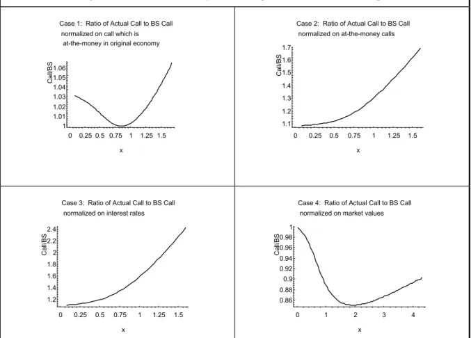
0, 0)_.

It is clear from Table 1 and Figure 6 that the asset prices and call price ratios of the actual and homogeneous-equivalent economies are very sensitive to the selected form of normalization. Depending on the normalization, some option prices may be found to be “underpriced” relative to the Black-Scholes case, and others to be “overpriced.” Still, as proved in Proposition 6, ultimately (that is, for a high enough strike price), the prices of the calls in our heterogeneous consumer economy will be larger than the Black-Scholes price in any “equivalent” homogeneous economy.

Figure 6: Four Different Normalizations

For each normalization, we show the ratio of the actual call prices to the call price in the “equivalent” homogeneous-consumer economy (this latter price is the Black-Scholes price).

0 0.25 0.5 0.75 1 1.25 1.5 x 1 1.01 1.02 1.03 1.04 1.05 1.06 Call/BS

at-the-money in original economy normalized on call which is Case 1: Ratio of Actual Call to BS Call

0 0.25 0.5 0.75 1 1.25 1.5 x 1.1 1.2 1.3 1.4 1.5 1.6 1.7 Call/BS

normalized on at-the-money calls Case 2: Ratio of Actual Call to BS Call

0 0.25 0.5 0.75 1 1.25 1.5 x 1.2 1.4 1.6 1.8 2 2.2 2.4 Call/BS

normalized on interest rates Case 3: Ratio of Actual Call to BS Call

0 1 2 3 4 x 0.86 0.88 0.9 0.92 0.94 0.96 0.98 1 Call/BS

normalized on market values Case 4: Ratio of Actual Call to BS Call

VI. Option delta with heterogeneous consumers

In the previous section we proved that when there is consumer heterogeneity in risk aversion, the option price for a sufficiently out-of-the money option is always larger in a heterogeneous consumer economy than the Black-Scholes price. In this section we explore the properties of the option delta in a heterogeneous consumer model. We prove that in a heterogeneous consumer environment, the option delta is always (for sufficiently high option exercise price) larger than the Black-Scholes delta.

The model employed in the previous sections had only two dates, 0 and 1. In order to explore option delta, we require a model which has intermediate periods. We build such a model in the most obvious way, assuming that the unit interval—the time between today (date 0) and the option’s maturity (assumed to be T = 1)—is divided into n subintervals. Since we have no analytic expression for the option delta, we approximate it by showing the sensitivity of the option price to the underlying stock price in some intermediate period.10

The option delta is the sensitivity of the option price to a change in the underlying asset price. In the BS model,

δ

_BS = N d

( )

1 . Assume that the options are

written on the market and that the time to maturity is T = 1. We write the _δ in our heterogeneous model as

δ

_HM

(

S X,

)

, where S is the market value. We prove the following proposition:

Proposition 7: For X sufficiently large,

δ

_HM

(

S X,

)

>

δ

_BS.

Proof (sketch): Consider a heterogeneous consumer model in which the consumers have relative risk aversions γ1 < γ2 < … < γH. The Black-Scholes option price is essentially an option price for some intermediate (“average”) risk aversion _γ1 < γ0 <

γH. It follows from Proposition 3 that the state prices in the heterogeneous consumer case can be regarded as derived from an “average” consumer whose relative risk aversion _γA_{(Y) is a decreasing function of aggregate terminal consumption Y, where}

γA_{(Y) → min (γ}

h) as Y →∞. It follows that the heterogeneous-model state price for Y

large enough is larger than the state price “Black-Scholes” (risk aversion γ0_{) case;} furthermore, the difference between the heterogeneous model and “Black-Scholes” state prices is an increasing function of aggregate consumption Y. Since the out-of-

10

Suppose for example that n = 50. Then for an intermediate period (say j = 20), our numerical model will calculate 21 pairs of option prices and market prices. Graphing these combinations will give the sensitivity of the option price to the underlying market price.

the money option prices payoffs only in these extreme states, this proves the proposition. ||

It is easy to illustrate the proposition, and it is also easy to see the necessity of X being large enough. In the example below, our two consumers are as before (risk aversions 1 and 7 and pure time preference _δ = 0.99). The option is highly out-of-the-money (X = 2). As predicted by the proposition, the difference between the HM option price and the BS price is an increasing function of S.

0.5 0.75 1 1.25 1.5 1.75 2 2.25 Stock price 0 0.05 0.1 0.15 0.2 0.25 ec n er eff i d

Actual Call Price minus BS

Figure 7

It is also easy to construct counter-examples to

δ

_HM

(

S X,

)

>

δ

_BS; this will occur for lower X, as in the example below, in which the option exercise price is X = 1. 0.5 0.75 1 1.25 1.5 1.75 2 2.25 Stock price 0.025 0 0.025 0.05 0.075 0.1 0.125 ec n er eff i d

Actual Call Price minus BS

The reason for this is clear: for a lower exercise price X the model prices can be considered to come from both low and high relative risk aversions. State prices in the heterogeneous consumer model will not be uniformly higher than the Black-Scholes state prices, and the resulting option deltas will exhibit behavior deriving from this property.

VII. Conclusion

People are different. Some are bold and daring, while others are overcautious. Such diversity is indeed one of the main economic rationales for Pareto-improving trade, and has been particularly emphasized in relation to speculative markets. In this paper we consider equilibrium option pricing in a simple two-period economy that is characterized by heterogeneity among agents. We demonstated that an economy in which agents have constant yet heterogeneous degrees of relative risk aversion will price assets as though it had a single “pricing representative” agent who displays

decreasing relative risk aversion. This result was shown to imply that the pricing kernel has fat tails and yields option prices which do not conform to the standard Black-Scholes formula. Solving for the implied volatility of either call or put options results in this case in a “smile” pattern, typical of those derived in practice. In addition we proved that the option delta for sufficiently out-of-the-money options is higher than the Black-Scholes delta.

Our explanation of heterogeneity as the source for this empirically observed phenomenon is simple and intuitive. It seems to fit Rubinstein’s (1994) interpretation of the “over-pricing” of out-of-the-money put options on the S&P 500 index as an indication of “crash-o-phobia”. Rubinstein’s term suggests that those who seek to hold out-of-the-money put options as protection against crashes are characterized by relatively high risk aversion or by subjective probability assessments with a relatively high (possibly unreasonable) weight on low market outcomes. If one were to assume that all investors share the same attitude towards risk and probability beliefs with regard to market crashes, there would be no explanation why some investors hold these extreme put options, while others write them. In addition, the very complexity of the implied binomial tree that Rubinstein derives suggests to us that it is likely to be the equilibrium outcome of a complex interaction among diverse investors, rather than to reflect uniform attitudes towards risk shared unanimously by all investors. While it is convenient to portray the economy through the construct of a fictitious “representative” investor, this convenience should not blind us to ignore the serious aggregation problems that are involved by such a construct, or to regard as innocuous the practice of endowing the fictitious “representative” investor with preferences and

probability beliefs that may be “reasonable” only for the actual investors in the economy.

REFERENCES

Bick, Avi (1987). “On the Consistency of the Black-Scholes Model with a General Equilibrium Framework.” Journal of Financial and Quantitative Analysis 22 (September), pp. 259-276.

Bick, Avi (1990). “On Viable Diffusion Price Processes of the Market Portfolio.”

Journal of Finance 45 (June), pp. 672-689.

Breeden, Douglas T. and Robert H. Litzenberger (1978). “Prices of State-Contingent Claims Implicit in Option Prices.” Journal of Business 51 (October), pp. 621-652.

Brennan, Michael J. (1979). “The Pricing of Contingent Claims in Discrete Time Models.” Journal of Finance 34 (March), pp. 53-68.

Constantinides, George, M. (1982). “Intertemporal Asset Pricing with

Heterogeneous Consumers and without Demand Aggregation.” Journal of Business 55 (April), pp. 253-267.

Cox, John C. and Mark Rubinstein (1985). Options Markets. Prentice-Hall. Franke, Guenter, Richard C. Stapleton, and Marti G. Subrahmanyam (1996), “Why

are Options Expensive?” mimeo.

Heaton, John and Deborah Lucas (1995). “The Importance of Investor Heterogeneity and Financial Market Imperfections for the Behavior of Asset Prices.”

Carnegie-Rochester Conference Series on Public Policy, Vol 42 (June), pp. 1-32.

He, Hua and Hayne Leland (1993). “On Equilibrium Asset Price Processes,” Review of Financial Studies, 6, pp. 593-617

Hirshleifer, Jack and John G. Riley (1979). “The Analytics of Uncertainty and Information: An Expository Survey.” Journal of Economic Literature 17 (December), pp. 1375-1421.

Kennickell, Arthur B. and R. Louise Woodburn (1992). “Estimation of Household Net Worth Using Model-Based and Design-Based Weights: Evidence from the 1989 Survey of Consumer Finances,” Board of Governors of the Federal Reserve System, manuscript.

Kirman, Alan P. (1992). “Whom or What Does the Representative Individual Represent?” Journal of Economic Perspectives 6 (Spring), pp. 117-136.

Leland, Hayne (1980). “Who Should Buy Portfolio Insurance?” Journal of Finance

35, pp. 581-594.

Lucas, Robert E. (1978). “Asset Prices in an exchange economy,” Econometrica 46, pp. 1429-1445.

Mankiw, N. Gregory (1986). “The Equity Premium and the Concentration of Aggregate Shocks,” Journal of Financial Economics 17, pp. 211-219 Mankiw, N. Gregory and Stephen P. Zeldes (1991). “The Consumption of

Stockholders and Nonstockholders,” Journal of Financial Economics, 29 (March), pp. 97-112.

Mayshar, Joram (1983). “On Divergence of Opinion and Imperfections in Capital Markets.” American Economic Review 73 (March), pp. 114-128.

Ross, Stephen, (1976). “Options and Efficiency,” Quarterly Journal of Economics 90

(February), pp. 75-89.

Rubinstein, Mark E. (1974). “An Aggregation Theorem for Securities Markets.”

Journal of Financial Economics 1, pp. 225-244.

Rubinstein, Mark E. (1976). “The Strong Case for the Generalized Logarithmic Utility Model as the Premier Model of Financial Markets.” Journal of Finance, pp. 551-571.

Rubinstein, Mark E. (1976). “The Valuation of Uncertain Income Streams and the Pricing of Options.” Bell Journal of Economics 7 (Autumn), pp. 407-425. Rubinstein, Mark E. (1994). “Implied Binomial Trees.” Journal of Finance 59

(July), pp. 771-818.

Shafer, Wayne and Hugo Sonnenschein (1982). “Market Demand and Excess Demand Functions.” Handbook of Mathematical Economics, Volume II, K.J. Arrow and M.D. Intrilligator (eds.), pp. 671-693.

Sharpe, William F. (1970) Portfolio Theory and Capital Markets. New York: McGraw-Hill.

Shefrin, Hersh (1996). “Behavioral Option Pricing.” mimeo.

Stapleton, Richard C. and Marti Subrahmanyam (1984). “The Valuation of Options When Asset Returns are Generated by a Binomial Process.” Journal of Finance 39 (December), pp. 1525-