Applicability and accuracy of quantitative
forecasting models applied in actual firms
A case study at The Company
Master of Science Thesis
in the Management and Economics of Innovation Programme
JOHAN EGNELL
LINNEA HANSSON
Department of Technology Management and Economics
Division of Innovation Engineering and Management
CHALMERS UNIVERSITY OF TECHNOLOGY Göteborg, Sweden, 2013
MASTER’S THESIS E 2013:115
Applicability and accuracy of quantitative forecasting
models applied in actual firms
A case study at
The Company
JOHAN EGNELL LINNEA HANSSON
Tutor, Chalmers: Jan Wickenberg
Department of Technology Management and Economics
Division of Innovation Engineering and Management
CHALMERS UNIVERSITY OF TECHNOLOGY Göteborg, Sweden 2013
Applicability and accuracy of quantitative forecasting models applied in actual firms Johan Egnell and Linnea Hansson
© Johan Egnell and Linnea Hansson, 2013
Master’s Thesis E 2013:115
Department of Technology Management and Economics
Division of Innovation Engineering and Management
Chalmers University of Technology SE-412 96 Göteborg, Sweden Telephone: + 46 (0)31-772 1000
Chalmers Reproservice Göteborg, Sweden 2013
Abstract
Taking off from an in-depth case study, this thesis deals with the concept of business forecasting. Business forecasting is the task of predicting future trends and demand in order for managers to make better decisions. Business forecasting as an academic subject has been studied extensively, and researchers have proposed numerous methods on how companies should approach forecasting effectively. A lion share of the methods studied by researchers involves manipulation of historical data by the use of quantitative models. Quantitative models are based on the assumptions that patterns can be found in historical data, and that the past pattern can be used to forecast future pattern.
The Company is a global B2B manufacturing firm with operations in more than 100 countries. As of today, their forecasting is constructed locally in each country through a judgmental approach where managers use their experience to estimate future order intake. This thesis describes how experiments were set up where the accuracy of a number of quantitative forecasting models was compared to the accuracy of the judgemental forecast.
The thesis makes three main theoretical contributions. Firstly, the findings of the thesis support the claim made by other researchers that quantitative models, on average, perform better compared to judgmental forecasts. The results of the experiments show that a quantitative approach to forecasting outperforms the judgmental forecast constructed by The Company with 50%.
Secondly, the result of the thesis show that a combination of quantitative models improve the forecasting accuracy compared to each of the individual models used in the combination. This is believed to be caused by the inherent bias within each model that is smoothed out when combining a number of different quantitative models.
Lastly, the authors of the thesis argue that the quantitative models that others researchers study and propose may be too complex to be of any use to those firms that wish to construct and control their own forecasting model. Many models, such as the ARIMA-models, require know-how on statistics and econometrics that are hard to find in many firms. Research on business forecasting is however relevant in the sense that complex models will eventually become available to firms in commercially software packages, making research on business forecasting relevant for actual firms.
Acknowledgements
Firstly, we would like to extend our gratitude to Professor Jan Wickenberg, whom in the role as tutor has guided us away from the sins of improper methodology and wrongful purposes. Jan also deserves recognition for his excellent work as lecturer and examiner at Chalmers University of Technology. We consider his course among the best, a statemenmt we know for sure that our fellow classmates agree with.
Secondly, we would like to thank Professor Patrik Jonsson for his guidance during the initial stages of this thesis. When we were stumbling in the dark, it was utter
happiness when Patrik lit the candle.
Finally, to our anonymous supervisor at The Company, your help was invaluable, and our gratefulness unmeasurable.
Table of content
1.
Introduction ... 1
1.1. Background ... 1 1.2. Purpose ... 2 1.3. Delimitations ... 2 1.4. Thesis outline ... 32.
Literature review ... 4
2.1. Background and history of business forecasting ... 4
2.2. Quantitative forecasts ... 4
2.2.1 Decomposition ... 5
2.2.2 Identifying outliers ... 7
2.2.3 Quantitative forecasting methods ... 8
2.2.4 Accuracy of quantitative forecasts ... 14
2.3. Combination of quantitative forecasting methods ... 15
2.4. Measures of forecasting accuracy ... 16
2.4.1 Scale-dependent measures ... 16 2.4.2 Scale-independent measures ... 16 2.4.3 Relative errors ... 17 2.4.4 Relative measure ... 18 2.4.5 Scaled errors ... 18 2.5. Judgmental forecasts ... 19
2.5.1 Judgmental forecasting methods ... 19
2.5.2 Accuracy of judgmental forecasts ... 20
2.6. Combination of judgemental forecasts and quantitative methods ... 21
2.7. Theoretical framework - Summary ... 22
3.
Method ... 23
3.1. Scope and general outline of the work conducted within this thesis ... 23
3.2. Literature review ... 26
3.3. Data collection... 26
3.3.1 Quantitative data ... 26
3.4. Qualitative data ... 27
3.4.1 Validity in qualitative interviews ... 27
3.5. Experiments ... 28
3.5.1 Forecasting methods ... 29
3.5.2 Measurements of forecasting accuracy ... 30
3.5.3 Identifying outliers ... 31
4.
Empirical findings – The Company ... 32
4.1. The Company – general information, products and market characteristics .. 32
4.2. Current forecasting processes at The Company ... 32
4.2.1 UK ... 33
4.2.3 Germany ... 34
4.3. Evaluation of forecast made by The Company ... 34
4.4. Data decomposition ... 36
4.4.1 Autocorrelation ... 37
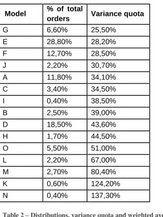
4.4.2 Model split ... 38
4.5. Accuracy of quantitative models ... 39
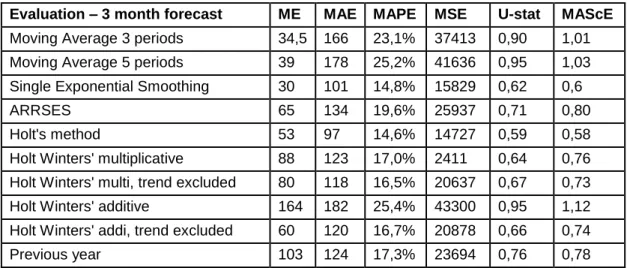
4.5.1 Accuracy of quantitative models – three months forecast ... 39
4.5.2 Accuracy of quantitative methods – six months forecast ... 40
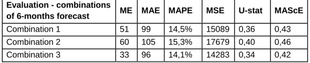
4.5.3 Combination of quantitative forecasts ... 40
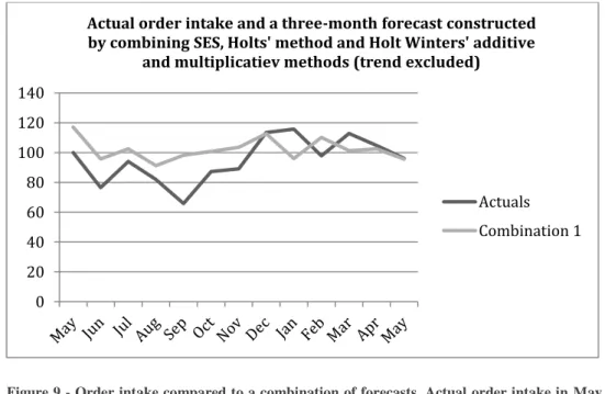
4.6. Comparison between actual forecasts made by The Company and a combination of quantitative forecasting models ... 42
5.
Discussion ... 44
5.1. Empirical findings compared to Hypotheses identified in academic literature 44 5.2. Do researchers study forecasting methods that are too statistically complex, and demand too much resource to be of any use for actual firms? ... 45
6.
Conclusion ... 49
7.
Bibliography... 50
1
1.
Introduction
This chapter gives an introduction to the subject of business forecasting, followed by the purpose of the thesis. Furthermore, the delimitations and general outline of the thesis are presented.
“Tell us what the future holds, so we may know that you are gods”
(-Isaiah 41:23 ) Background
Predicting the future has been a part of human lives since the dawn of humanity, and many different methods have been used in the past, some of them being fairly dysfunctional. In ancient Babylon, the future was predicted by the amount of maggots in a rotten sheep’s liver while people in the Nordic countries turned to patterns in the fire to foretell future events.
As the prophet Isaiah expressed it in the beginning of the chapter, a person whom excelled at foretelling was considered to possess godlike skills, and for those excelling in foretelling the future, the opportunity of fortune and fame was considerable. Today, the usage of dysfunctional methods and the godly context has deteriorated, but the possibility of fortune and fame is still present for those that forecast accurately. Consequently, bad forecasting might have serious consequences. An example of forecasting going wrong are the alleged words of Ken Olsen, president of Digital Equipment Corporation (DEC) in 1977: “There is no reason for any
individual to have a computer in their home”. Subsequently, DEC entered the personal computer market too late and struggled until they were acquired in 1992. For businesses working in the global and competitive environment of today, the need of accurate forecasting is as important as ever before. Short lead-time, just-in-time-delivery and cost effectiveness are all drivers of success that are directly linked to an understanding of customer demand, making accurate forecasts an integral part of a firm’s general competiveness.
Business forecasting is defined as a management tool that aims at predicting the uncertainties of business trends in order for managers to make better decisions (Hanke & Wichern, 2005). A quantitative approach to business forecasting relies heavily on statistics and the manipulation of historical data. Quantitative forecasting has been studied extensively in the last decades, and various methods on how to manipulate and interpret data have been proposed.
Quantitative forecasting methods have been found to produce more accurate forecasts than judgemental, or qualitative, forecasts (Pant & Starbuck, 1990). However, despite
2
the advanced computers we have today, and the constant development of quantitative models and methods, most scholars emphasises the involvement of logic thinking and judgemental adjustment to quantitative forecasts (Pant & Starbuck, 1990; Hanke & Wichern, 2005; Fildes, et al., 2009).
There is a scarcity of resources within all firms, and companies cannot undertake all projects (Maylor, 2010, p.56). Researchers studying business forecasting rarely take this fact into account, as the methods researchers construct tend to become more and more advanced, and thus more costly (Makridakis & Hibon, 2000). The risk associated to researchers not taking the boundaries of resource-reality of actual firms into consideration might be that the research becomes focused on forecasting methods that have few practical implications, as they are too expensive and too difficult to implement in actual firms. As the actual definition of business forecasting is rather practical, one might also argue that the scholarly community is moving away from the actual object the community claims to be studying.
Purpose
The purpose of this report is to contribute to the existing knowledge on business forecasting through a case study. In the case study, different quantitative forecasting models are applied on historical data in order to compare them to the judgemental forecasting processes used today at The Company.
The findings of the case study will be compared to hypotheseses identified in the academic literature. The thesis also aim at contributing theoretically by discussing if the quantitative forecasting models studied and proposed by other researchers have limited practical implications, as the methods might be too statistically complex to be of any use of actual firms.
Delimitations
When given the task to identify a quantitative forecasting model for The Company,
the model needed to be easy to understand, easy to implement and easy to explain. The model also needed to be simple enough so that changes in the model, (e.g. values of variables), could be made in-house, and would not require experts/consultants. The improvement in forecasting accuracy also needed to be significant; otherwise changes in the forecasting process would be unnecessary when considering the cost/benefits of changing the current processes.
The Company has five differentiated product groups according to their respective field of application. We were asked to produce a forecast for one of the groups; Product group 1.
3 Thesis outline
This thesis is divided into six chapters. Chapter 2 presents an outline of the research on business forecasting that affects this thesis. Emphasis is placed on the introduction of different forecasting models, data decomposition, judgemental forecasts and measures of accuracy. The methods used in order to reach a valid conclusion are presented in chapter 3.
The empirical findings of the thesis are introduced in Chapter 4, being briefly introduced by a short presentation of The Company and their current forecasting processes. Chapter 5 presents a discussion regarding the relation between the theoretical and the empirical findings in order to fully reach the purpose of the thesis. Lastly, the conclusion drawn in from the thesis, along with suggestions regarding further research is found in chapter 6.
4
2.
Literature review
This chapter include a comprehensive guide to the research done within the field business forecasting. Initially, a short introduction of the history and development of business forecasting will be given, followed by a presentation of the research related to the scope and aim of this thesis, such as different quantitative and judgmental forecasting methods and methods on how to measure forecasting accuracy.
“Prediction is very difficult, especially about the future.”
(- Niels Bohr, as quoted in Pant & Starbuck, 1990, p. 433)
Background and history of business forecasting
When business forecasting was introduced as a subject of academic interest, the method used most widely within the business sector was exponential smoothing methods. A practitioner, Robert G. Brown, introduced the methods in the late 50s (Lapide, 2009). These exponential smoothing methods still live on today. Later, more advanced methods taking seasonality and trend into account were brought forward in the 60’s and 70’s by scholars such as Holt (trend) and Winter (seasonality and trend) (Lapide, 2009).
As managers later understood that actions such as promotional activities, competitor action and product introduction would shape and create demand, these variables needed to be understood and incorporated into the forecasts. One method to incorporate explanatory variables was the ARIMA-model. Pioneers within the field of ARIMA-models were statisticians George Box and Gwilym Jenkins who 1970 created the Box-Jenkins methodology to find the best fit of a model in order to forecast (Lapide, 2009).With the introduction of computers, more advanced forecasting measures has emerged. In the latest of the M-competitions, were different forecasting methods are compared, seven (out of 24) were software-run commercially available packages (Makridakis & Hibon, 2000).
Quantitative forecasts
The features of quantitative forecasting models vary greatly, as they have been developed for different purposes. The results are a number of techniques varying both in complexity and structure. However, a common notion is that quantitative forecasts can be applied when three conditions are met (Makridakis, et al., 1998, p. 9):
1. There is information about the past 2. The information can be quantified
5
3. It can be assumed that the past pattern will reflect the future pattern.
Once it has been specified that the data available respond well to the three conditions above, the actual recognition of an appropriate forecasting technique can begin. This is mainly done by initially investigating the data, a task known as Decomposition
(Hanke & Wichern, 2005, pp. 5-7). 2.2.1 Decomposition
Quantitative forecasting methods are based on the concept that patterns in historical data exist, and that this pattern can be used when predicting future sales (Makridakis, et al., 1998). Most of the forecasting methods break down the pattern into components, where every component is analysed separately. This breakdown of pattern is also called the decomposition of a pattern. Decomposition is usually divided as follows:
Where:
Yt = the time series value at period t
St = the seasonal component at period t
Tt = the trend-cycle component at period t
Et = the error component at time t
The method that calculates the time series value can have an additive or a multiplicative form. The additive form is appropriate when the magnitude of the seasonal fluctuations does not vary with the level of the series. The multiplicative form is thus appropriate when seasonal fluctuations increase and decrease with the level of the series.
The additive decomposition equation has the form:
While the multiplicative decomposition has the form:
Seasonally adjusted data
Seasonally adjusted data can easily be calculated by subtracting the seasonal component from the additive formula, or by dividing it from the multiplicative formula. Calculating the seasonal component can be done in many ways, and involves comparing seasonal data to the average value. For example, if the average value over a year is 100, while the value for January is 125, the seasonal component is 25 for an additive approach, and 1.25 for a multiplicative approach.
6
Once the data has been seasonally adjusted, only the trend-cycle and irregular components remain. Most economic time-series are seasonally adjusted as seasonality variations are generally not of primary interest. When the seasonally adjusted component has been removed, it is easier to compare values to each other.
Trend adjusted data
Trend-cycle components can be calculated by excluding the seasonality and irregular component. There are many different methods to identify a trend-cycle but the basic idea is to eliminate the irregular component from a series (as the seasonality component has already been removed – see above) by smoothing historical data. The simplest and oldest trend-cycle analysis model is the moving average model. There are several different moving average models such as simple moving average, double moving average and weighted moving average (Makridakis, et al., 1998)
Error adjusted data
Simple moving average assumes that observations that are adjacent in time are likely to be close in value. Through a smooth trend-cycle component, simple moving average will eliminate some of the randomness that occurs (Makridakis, et al., 1998). When using simple moving average the first thing to be decided is the order of the moving average. Order means how many different checkpoints to use in the analysis. Common orders to use are 3 or 5. The more order of numbers included, the smoother forecast you get. The likelihood of randomness in the data will also be eliminated with a large number of orders. Simple moving average can be used for any odd order. Order is defined as k, and the trend cycle component by the use of simple moving average is computed as:
∑
where
t is the period which trend component is estimated, and t is also the centred number. This means that in a three-order average, the third is the period that follows the period that is being measured. Every new calculation drops the oldest number and include a new number, that why that is called moving average. Because of this, it is not possible to calculate the trend-cycle in the beginning and in the end of a time series. To overcome this problem a shorter length moving average can be used in the initiating phase, which means that the first number can be estimated by using an average of m.
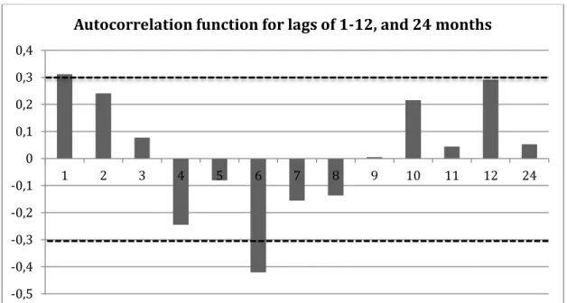
7 Autocorrelation
Another way to decompose a data series is to perform an autocorrelation analysis. Autocorrelation analysis allows you to investigate patterns in the data by studying the autocorrelation coefficients. The coefficient shows the correlation between a variable lagged a number of periods and itself. The autocorrelation can be used to answer four questions regarding patterns in a time series (Hanke & Wichern, 2005):
1. Is the data random? 2. Do the data have a trend? 3. Is the data stationary? 4. Is the data seasonal?
The autocorrelation coefficient (rk) is computed as:
∑ ∑
Where k is the lag and Y is the observed value.
If rk is close to zero, the series can be assumed to be random. That means that for any
lag k the series are not related to each other.
If rk is significantly different from zero for the first time lags and then slowly drop
towards zero as the number of lags increases, the series can be assumed to have a trend.
If rk reappears in cycles, the series can be assumed to have a seasonal pattern. The
coefficient will reoccur in a pattern as for example four or twelve lags. A seasonal lag of four means that the data-series is quarterly, while a significant value twelve means that the series is yearly.
The definition of autocorrelation close to zero is that the distribution of the autocorrelation coefficient is approximated as a normal distribution with a mean of zero and has an approximated standard deviation of 1/√n (Hanke & Wichern, 2005). To calculate the critical values, Makridakis et. al. (1998) propose to use a 95% confidence interval, meaning that 95% of all samples of autocorrelations coefficients will be within ±1.96/√n for the series to be counted as close to zero.
2.2.2 Identifying outliers
An important aspect of setting up a quantitative forecasting model is that of identifying outliers. Outliers are values outside a lower and upper limit (typically 95% confidence interval around the mean of the data set) that depend on an external factor. In business forecasting, an outlier usually means that seasonal factors (such as the end of a budget year, or vacations) or single events (large tender orders from a big
8
company) for a specific month/week/day affect the order intake heavily. The extreme value in order intake will not reflect normal demand, and should therefore not be considered when setting up quantitative forecasting models (Hanke & Wichern, 2005, pp. 72-74).
Consider a firm that has a price increase in December each year. The price increase makes the demand for the company’s product increase by 200% in November. If the November value should be used when forecasting future demand, the forecast will be too high, as future demand will depend on a data set that doesn’t reflect normal demand. Researchers have identified numerous ways of identifying outliers. Two methods are called trimming and winsorizing. When trimming data, the top and bottom values are excluded determined by a fixed value in per cent. For example, a 10 per cent trimming means that the top 5 percent and the bottom 5 percent are discarded from the data set. Winsorizing is similar to trimming, but it replaces extreme values instead of discarding them. A 10 per cent winsorization means that the data below the 5th percentile of the data is set to the 5th percentile and the values above the 95th percentile is set to the 95th percentile (Jose & Winkler, 2008).
2.2.3 Quantitative forecasting methods
A major factor influencing the selection of forecasting method is what pattern that can be identified within the data. Depending on characteristics such as seasonality, trend and cyclical patterns in the data series, different models are better optimized to deal with the patterns found in the data. The concept of choosing a forecasting method is based on trial and error (Hanke & Wichern, 2005). The trial is set up by applying historical data to a forecasting model to measure how accurate the model would have forecasted. The forecasting method that produces the most accurate and the one with the least error will be used for the future (Hanke & Wichern, 2005).
This chapter will present a number of forecasting methods that are introduced by Makridakis, Wheelwright and Hyndman in their book Forecasting: methods and applications (1998). For further discussion regarding the choice of forecasting methods, please see chapter 3.
Moving averages forecast
Moving average is one of the most basic forecasting models. It uses the averages of the latest k periods of known data to forecast, which means that the model requires data to be stored from the k latest periods.
∑
9
Where is the forecast, and is the actual value at time t. The model is simple to understand and use but at the same time the model does not handle any trend or seasonality fluctuations.
Exponential smoothing methods
Exponential smoothing methods have the properties that recent values are given more weight in forecasting than the older observations. The methods use weighted average from past observations using weights that decay smoothly. There are several exponential smoothing methods and most of them don’t take seasonality or trend into account with the exception of Holt’s method, which identifies trend within a series, and Holt-Winters’ method, which involves three parameters taking smoothing factors, trend and seasonality into account.
Single exponential smoothing
Single exponential smoothing (SES) utilizes the forecast made for the previous period, in combination with the forecast error, to estimate future values. The form of SES looks as follows:
or,
In this form, the new forecast ( ) is the old forecast ( ) adjusted by α times the error of the old forecast. can in turn be substituted by:
This way, the most recent observation is given the largest weight, the second most recent less weight and so forth. A small α will give little weight to the most recent observation (but still more weight than the second most recent observation), making the new forecast similar to the old forecast, giving the latest observation a small impact on the forecast. A big α represents a small number of historical data and a small α represents a large number of historical data. Therefore, a small value of α require a better optimized first value since it will influence the rest of the forecasts more than it would if α were large.
The initial problem of using SES is to optimize α. The optimal α should be chosen so that it minimizes the forecasting error. There are algorithms calculating the best α, but it is however quite simple to identify a good α simply by comparing a number of values between zero and one (Makridakis, et al., 1998, pp. 154-162).
10
Compared to moving average, single exponential smoothing lacks need of storage of historical data as you only need the old forecast and the most recent actual value, which makes SES easy to use when historical data is missing.
Adaptive-response-rate single exponential smoothing
A modification of SES is the adaptive-response-rate single exponential smoothing (ARRSES). Possible advantage with ARRSES, compared to SES, is that α can be modified as changes in data occur. ARRSES takes both a smoothed estimated forecast error and a smoothed estimated absolute forecast error into account. Except α, the ARRSES model use β as a parameter between 0 and 1 to calculate those two estimated errors.
As can be seen in the formulas, α depends on β. It is common that a small β is chosen, which means that α will not fluctuate very much. When using ARRSES, the forecast is completely automatic and together with the advantages of SES gives ARRSE useful when the data set shows no seasonality or no trend. As with SES, the variables α and β has to be optimized initially with regards to the forecasting error. Optimizing variables can either be done through a computerized algorithm, or by a matrix where the forecasting accuracy from using different values of α and β are placed in a matrix, thus highlighting what combinations produce accurate forecasts.
Holt’s linear method
Holt’s linear method is a method that takes trend into account and this method is found using two smoothing constants, α and β and following equations:
Lt denotes an estimate of the level of the series at time t and bt denotes an estimate of
11
There are a few different alternatives to estimate L1 and b1 in the initialization phase.
One is to set L1 =Y1, another is to use least squared regression on the first few values
of the series and b1 can be defined as the difference between Y1 and Y2 or as average
of the first few difference values of the series.
As for SES and ARRSES, α and β can be optimized by using a non-linear optimization algorithm with regards to minimizing the forecasting error.
Holt-Winters’ trend and seasonality method
Holt-Winters’ method is, in addition to Holt’s linear method, a method that takes both trend and seasonality into account. The equations for Holt-Winters’ method are similar to Holt’s equations; the difference being that there is an additional variable dealing with seasonality. The equations below are for Holt-Winters’ multiplicative method, the additive method is less common, but will shortly be presented later.
St denotes the seasonal component, and s is the length of seasonality while γ is the
seasonal factor.
In the initialization phase Ls, bs and Ss are being calculated as:
As for other methods, using a non-linear optimization algorithm can optimize α, β and γ.
Holt-Winters’ additive method is less common than the multiplicative method. The two methods look nearly the same, the difference is that seasonality is added and subtracted instead of taking products and ratios as in the multiplicative method.
12
The initializations values for Ls and bs are calculated the same way as for the
multiplicative method, while the initialization value for Ss is estimated as:
Box-Jenkins: ARMA and ARIMA models
ARIMA models are a class of models that produces forecasts based on a description of historical pattern in the data ARIMA stands for Autoregressive integrated moving average and are models used when the series is non-stationary, different from ARMA models that are used when data are stationary. Data is stationary when there are no changes in the mean or in variance over time, and vice versa for non-stationary data (Hanke & Wichern, 2005, pp.215-267).
ARIMA (p, d, q) has the notations of: AR: p = order of the autoregressive part I: d = degree of first differencing involved MA: q = order of the moving average part
The Box-Jenkins methodology is not a specific forecasting method per-se, but it is instead an iterative method to identify a fitting ARIMA model to the data set. The fitting is mainly done in three steps (see Figure 1). In the first step, model identification, the data is investigated in order to determine whether the data is stationary. This is done by looking at a plot of the time series, along with looking at an autocorrelation function of the data. If the time series is non-stationary, it can be converted to a stationary series by differencing. Differencing means that the original series will be replaced by a series of differences (between Yt and Yt-1) in order to
make the series stationary. This process of differencing represents the I (integral) in ARIMA (Hanke & Wichern, Business forecasting, 2005).
The second part of step 1 is to compare the autocorrelation function to a number of theoretical ARIMA models. Researchers have computed guidelines that show what forecasting models are appropriate depending on the look of the autocorrelation function. There are too many ARIMA and ARMA models to be described in this chapter, but most models include either an autoregressive component, a moving average component, or both.
13
The second step in the Box-Jenkins methodology is model estimation. Once a model has been identified in step 1, its variables have to be estimated. The variables are estimated by optimizing the variables with regards to minimizing the mean squared errors, as well as minimizing the variance of the errors (Hanke & Wichern, Business forecasting, 2005).
The third step is to check the adequacy of the model. This is done by checking the errors. An autocorrelations function of the error should be small, usually within 2 standard deviations from zero. Significant autocorrelations suggest that the data is non-stationary or contains seasonality, and therefore a new or modified model should be selected.
Postulate General Class of Models
Diagnostic Checking (Is the model adequate?) Estimate Parameters in Tentatively Entertained Model Identify Model to Be Tentatively Entertained Yes
Use Model for Forecasting No
14
2.2.4 Accuracy of quantitative forecasts
There have been a number of studies where different (quantitative) forecasting methods have been compared to each other. Makridakis and Hibon have led three competitions called M-competitions, where researchers all over the world were invited to construct a forecast from a given set of time series data. In the first M-competition held in 1982, 15 forecasting methods (and nine variations) computed forecast from 1001 real-life time series. The second competition, held in 1991 was designed to run on a real-time basis in collaboration with four companies designated to provide both data and to answer questions on factors and variables the participating researchers wanted to know more about (such as competitors, product mix etc.). The competition ran for two years and also involved estimating six macro-economic series. After one year, the researchers were allowed to change their forecasts. The findings from each of these two competitions were practically identical and were summoned by Makridakis and Hibon as (Makridakis, et al., 1993):
a) Statistically complex methods do not necessarily provide a more accurate forecast
b) The relative ranking of the methods varied when different methods were used to measure the forecast accuracy.
c) A combination of forecasts outperform, on average, the individual methods being combined
d) The accuracy of the methods varies according to the time horizon being forecasted
Despite these findings (which were validated by many of the participating researchers), theoretical forecasters have (according to Makridakis and Hibon) largely ignored this and continued to put effort into building more complex methods. A final attempt to settle the issue was made in 2000 when the M3 competition was launched, where 24 different models utilized 3003 different time series covering industry, micro, macro, finance, demographics, as well as yearly, quarterly and monthly data. The results from the M3 competition once again confirmed the previous findings from the M1 and M2 competition. These findings have been examined and confirmed by other researchers who have used the same set of data as the one used in the M-competitions; (Geurts & Kelly, 1986; Clemen, 1989; Flores & Pearce, 2000; Konig et al., 2005).
The reason why sophisticated and well-fitted models do not perform better than simple models is explained by Makridakis and Hibon (2000) by the fact that future data is usually never as predictable as quantitative models suggests and that past data cannot predict upcoming event and changes. The fact that sophisticated models are fitted against past events creates a bias within the model as the variables change with unforeseen and low predictability events such as competitor action, technological changes and macro-economic changes.
15
Combination of quantitative forecasting methods
Combining more than one forecast has been shown to reduce forecasting errors (Makridakis & Hibon, 2000; Ringuest & Tang, 1989). The improvement accuracy tends to greater be when the individual forecasts have poor accuracy themselves (Makridakis & Hibon, 2000). Researchers have tried to identify optimum ways of combining forecasts, but empirical studies has shown that the accuracy can be increased significantly simply by putting equal weight to a number of forecasts that is combined, or by a median combination method (Ringuest & Tang, 1989).
The general form of a combined forecast is:
Where: is the combined forecast,
is the forecast from the jth method, is the weight applied to the jth forecast,
n is the total number of forecasts available for combining
A simple average combined forecast is computed by putting equal weights to all forecast by dividing the weight with the total number of forecasts:
A median combined forecast is constructed by putting if the jth method yields the median value of the tested models. Otherwise, .
Ringuest and Tang (1989) write that taking historical forecasting experience into account when combining forecasts (which average and median combination doesn’t) can increase the accuracy even further. They suggest a combination that is built on the notion that a forecast that produced the most accurate forecast the previous period, is most likely to produce the most accurate forecast the following period. Thus the weight is computed as:
; if the forecast from the jth period produced the least forecasting error in the previous period.
and
; otherwise
16
; if the jth method was in bottom xth percentile the previous period.
and,
; otherwise
Measures of forecasting accuracy
There are many different ways of evaluating forecasting methods. Rob J. Hyndman and Anne B. Koehler have summarized many of the existing measures in an article published in 2006. The disadvantages and advantages of each method are also pointed out. They have divided the measures into five different groups: Scale-dependent measures, Scale-independent measures, relative error relative measures and scaled error measures.
2.4.1 Scale-dependent measures
Scaled-dependent measures are accuracy measures whose scale depends on the scale of the data. A scale-dependent measure is not preferable when comparing different data sets. Examples of the most commonly used scale-dependent measures are:
∑ √ ∑ ∑
Since RMSE and MSE will be more sensitive to extreme values than MAE or MdAE, MAE and MdAE might be better when measure forecasting accuracy for a volatile observed data set.
2.4.2 Scale-independent measures
Scaled-independent measures are accuracy measures whose scale does not depend on the scale of the data. A scale-dependent measure can be preferable when comparing
17
across data set (Hyndman & Koehler, 2006). Examples of the most commonly used scale-independent measures are:
∑ ( ) √ ∑ √ ∑
The most common measure is MAPE, and many textbooks and articles recommend MAPE when comparing the accuracy of different forecasts, largely because of the variables relevance in statistical modelling (Hanke & Reitsch, 1995, p. 120; Bowerman, et al., 2004, p. 18). Other researchers point out that using scale-independent measures there will appear some difficulties when time series contains a zero-value, and for Yt is close to zero (Makridakis, et al., 1998, p. 45). Coleman and
Swanson (2004) argue that logarithmic scale can help measures based on percentage errors to be less skewed.
2.4.3 Relative errors
Relative error measures are an alternative way of scaling the data by dividing each error by an error obtained using a different forecasting method. The error obtained from the method of comparison method is denoted with a*. The usage of relative error is usually a way to compare how different forecasting methods perform against one single method (usually a naïve1 method). The different forecasting methods are then ranked according to their performance against the method of comparison. Examples of the most common used relative error measures are:
1 Naïve method is when the last known actual is used to forecast future all future values (Makridakis, et
18
∑
( )
The greatest disadvantage with relative error is that the models have a statistical distribution with undefined mean and infinite variance (Hyndman & Koehler, 2006).
2.4.4 Relative measure
An alternative to use relative error is to use a relative measure. This is also a method to compare different forecasting method with each other, but instead of comparing errors, a relative measure compares the actual measurements of accuracy. For example, MAE of a forecast can be compared with the MAE for a benchmarked forecast to show how different methods perform against a one single method (again, a naïve method is usually chosen as the method of comparison).
When the benchmarked forecast is a naïve method and the relative measure value is RMSE, the method is called Theil’s U statistics (Makridakis, et al., 1998). When Theil’s U statistic (or any other relative measure) gives a value less than one, it indicates that the forecasting method is better than a naïve method, and vice versa.
2.4.5 Scaled errors
Scaled error uses a meaningful scale when measure the forecast accuracy and it is also widely applicable compared to relative errors with undefined mean and infinite variance and relative measures which only can be computed when there are several forecasts on the same series (Hyndman & Koehler, 2006).
Scaled error is defined as:
∑
Using this definition of scaled errors, different comparison variables can be defined as for example:
√
19
Hyndeman and Koheler propose that measures based on scaled errors should be the standard approach for measuring forecasting accuracy. They have also applied a scaled error measure to the M3-competition, showing that the results it provided were more consistent with the actual conclusions of the M3 competition. Hyndeman and Koheler also suggest that it is less sensitive to outliers and more easily interpreted than RMSSE, and less variable on small sample than MdASE. In the latest of large forecasting competition held in 2010, tourism data was used, the researchers who set up the competition endorsed the opinion of Hyndman and Koehler; that MAScE should replace MAPE as the standard measure of forecast accuracy (Athanasopoulos, et al., 2011).
A value of MASE greater than one shows that the proposed forecast, on average, gives smaller errors than the benchmarked forecast, and vice versa.
Judgmental forecasts
Even if a firm has the ambition of using quantitative models as the primary mean to forecasting, there should always a measure of judgement involved in the forecasting process (Hanke & Wichern, 2005, p. 463). Good judgement is required when deciding if the data that is available is relevant. The interconnection between the future and the past might change (e.g. change of technological base in society) and thus the variables used in the model will not be optimized to predict future outcome. In those cases, theoretical models must be changed according to judgement and knowledge of the different market factors.
There is a wide range of possibilities on how a firm can utilize judgemental adjustments to forecasts. On one end, there is the possibility of firms’ historical data series, and adjustment is a very small part of the forecasting process. On the other end, circumstances might make it impossible to use a quantitative model, or the use of one might not be practical. Circumstances that make the use of theoretical models impossible might be that there are no data available, or that the analyst’s opinion is that the historical data is directly irrelevant to future demand (Harvey, 1995).
2.5.1 Judgmental forecasting methods
The methods described below are not subject to empirical testing later in this report. Instead, they are presented simply to show alternatives to quantitative forecasts that are strictly based on judgement.
The Delphi Method
Group dynamics is a critical issue when a group of people is asked to jointly reach a consensus about the future. The result of an exercise like that is that the group will reach “consensus”, even though all participants may not agree to the decision,
20
because of high-ranking members or of vocal members of the group (Hanke & Wichern, 2005, p. 464). One method to avoid the aspects related to group dynamics from the forecasting process is the Delphi method. Initially, members of the group reply in writing what they’re thought are on the questions posed by an investigation team. The opinions and then summed up and e-mailed to all members who can answer and defend or change their opinion. This usually goes on for another two or three round until the investigation feels that they have information on all aspects of the future (Rowe & Wright, 1999).
Bottom up/ Top down forecasts
Bottom-up and Top-Down forecasts are two sides of the same judgmental-forecasting-coin. The forecast is made in-house by either salespersons (bottom-up) or managers (top down) to estimate sales. Top-Down forecasts is usually believed to be more focused on the general knowledge of the business, while bottom-up forecasts are believed to have an advantage because of salespersons knowledge on the local market (Kahn, 1998).
2.5.2 Accuracy of judgmental forecasts
Research has shown that whenever historical data is available, the interference of judgemental modifications on average reduces the accuracy of the forecast (Jain, 1990; Flores & Pearce, 2000). Graham and Harvey (1996) showed that three quarters of all newsletter recommendations made by (supposedly) knowledgeable professionals for investments on the financial market performed worse than a random selection of stocks. Professional managers investing in stocks and funds also consistently underperform when compared to the S&P 500 index (Makridakis, et al., 1998, p. 485). A common explanation to this finding is attributed to bias on the part of the forecaster, possibly because of a tendency to be overly optimistic or pessimistic (Graham & Harvey, 1996). It has also been shown that a judgemental component within a forecasting process increases the cost of forecasting (Makridakis, 1986, p. 45).
A number of judgemental forecasts made for areas other than financial investments have been shown to perform worse than a naïve method. Salesperson’s forecasts have for example been shown to be notoriously inaccurate (Walker & McKlelland, 1991; Winklhofer, et al., 1996; Makridakis, et al., 1998). Salespeople’s forecasts fluctuate considerably depending on the mood of the salespeople and whether the rate of success of sales calls made close before forecasting (Walker & McKlelland, 1991). There is also a possibility that salespeople are rewarded if selling more than their target, which increases bias. At the same time, sales managers want to set high targets as motivation for the salespeople, thus adjusting the forecasts upward.
Management forecasts are much as likely as being inaccurate as salespeople forecast. Managers tend not to see how competitive threats or new technologies will affect the
21
market, and (Walker & McKlelland, 1991) has shown that managers are overoptimistic and that they have difficulties setting personal and political interests aside. In line with the general knowledge on judgemental forecast, management forecast are inferior to statistical models, as long as data is available. The same result has been observed when researchers have compared “expert” (business analysts, researchers etc.) forecasts with those if statistical models (Makridakis, et al., 1998, p. 492). Another interesting aspect of judgemental forecasting is that biases cannot be avoided by making decisions made in groups. Instead, groups amplify the effect of bias (Janis, 1972) as members become supportive of the leader and each other. Another problematic aspect of group decisions is that responsibility for the decision cannot be traced back to one single individual.
Combination of judgemental forecasts and quantitative methods
The notion of judgemental forecasts being inferior to statistical models has hopefully become clear to the reader at this point. With that said, salespersons and managers do possess valuable information that could greatly improve a firm ability to estimate future demand. One way to take advantage of the objectiveness of theoretical models, while capitalizing from judgemental information and management knowledge is a procedure called anchoring (Makridakis, et al., 1998). When anchoring, a number of key people are shown the forecast made by the quantitative model. To this, they add or subtract a percentage to the forecast depending on circumstances and variables they feel that the theoretical model does not take into account. The proposed changes must be explained and the factors involved must be written down. The adjustments are made anonymously in order to avoid being influenced by high-ranking members of the group.
An investigation Fildes et. al. (2009) of more than 60,000 quantitative forecasts and their accuracy made by four companies, known as being good at forecasting, showed that 80 per cent of all forecasts made had a judgemental adjustment to the initial forecast calculated by a computer. The result of the adjustment was three times out of four a more accurate forecast. The investigation shows that larger adjustment increase accuracy while small adjustments tend to decrease the accuracy. This is explained by the fact that large adjustments are based on specific knowledge of larger events (marketing campaigns, price increase etc.) while smaller adjustments tend to be based more on “gut-feeling”. When studying positive and negative adjustment where positive adjustment decreases the accuracy and vice versa for negative adjustment. Fildes et al. (2009) explain this attribute by a general over-optimism in management judgement.
Other circumstances when judgemental adjustments increase the accuracy are when the volatility of sales is high. (Sanders & Ritzman, 1992) has shown that a coefficient of variation (ratio of the standard deviation of the data divided with the overall mean) reached 30 per cent, adjustments started to increase the accuracy. As the volatility
22
increases, the accuracy has been shown to increase even further. But, this relation is only true as long as the volatility in a series does not reflect unanticipated events (O'Connor, et al., 1993).
Reasons for judgemental adjustment decreasing the accuracy include the fact that analysts adjust forecasts based on unreliable data, and that adjustments (with or without reason) tend to give the analyst more confidence in the forecast (Harvey, 1995; Kottemann, et al., 1994).
Theoretical framework - Summary
In order to contribute to the existing knowledge base on business forecasting, three hypotheses has been identified that will be compared to the empirical findings made within this thesis:
H1: Quantitative forecasts outperform, on average, judgmental forecasts.
H2: A combination of forecasting methods will increase the accuracy when compared to the individual methods that.
H3: The relative ranking varies depending on which accuracy measure through which the forecasting method is measured.
A fourth hypothesis has been identified in the academic literature, but it will not be compared to any empirical findings, as an empirical investigation on how much the accuracy increases because judgemental adjustments to a quantitative model. It will instead be discussed in relation to the capabilities of key personnel at The Company.
23
3.
Method
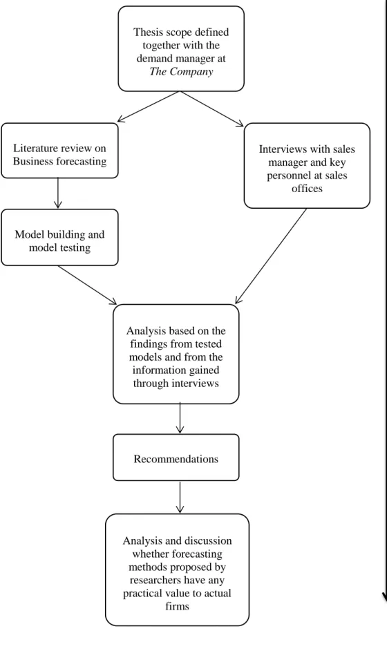
This section provides a description on how the report was conducted. In order to reach the objective of this thesis the methodology was divided into four distinct sections:
A literature review on the subject was conducted in order to gain enough knowledge on the subject to be able to draw valid conclusions when looking at the results of the experiments and from the interviews. Knowledge on the subject was also crucial when setting up experiments, as well as the outline of the interviews (Dalen, 2007, p. 12).
Secondly, we collected data on The Company. The data collected consisted of both quantitative and qualitative data. Examples of quantitative information are sales figures, external order intake and previous forecast made by The Company. Qualitative data was mainly collected through interviews with personnel within the organization.
An effort has been made to “clean” the quantitative data from outliers in order to optimize the third step of the process, which was to apply historical data on different forecasting models presented in the academic literature to see which would have the most potential to increase the forecasting accuracy.
The last section in the methodology was to discuss the empirical findings in relation to the theoretical framework as well as the overall purpose and aim of the thesis.
Scope and general outline of the work conducted within this thesis
The scope of the thesis was discussed at an initial meeting at The Company. It was decided that the thesis would study what the current forecasting process at The Company looks like, and to investigate whether a quantitative forecast based on historical data could improve the current forecasting process. Within the scope, it was also decided that the quantitative method that were to be studied, needed to be simple enough for The Company to implement them without having to hire consultants to do it, or spending much time understanding the underlying theory of the forecasting method. The decision which methods to test were decided jointly by the authors, the demand manager and the data intelligence manager.
Contact was taken with Patrik Jonsson, professor in Operations and Supply Chain Management at the Division of Logistics and Transportations at Chalmers University of Technology. He was of great help much help by proposing books and articles. Prof. Jonsson also explained the methodology behind testing and evaluating different forecasting methods. It is believed that without his help, the result of the thesis would not have been as valid as otherwise.
24
Information on the current forecasting process was mainly gained through interviews with the demand manager, and with sales managers and business controllers at various sales offices in Europe.
To test whether a quantitative forecasting method is a mean to increase forecasting accuracy, an extensive literature review on business forecasting was launched. Information gained from textbooks and articles published in scientific journals were used to construct a number of different quantitative forecasting models in order to identify methods that could increase the accuracy of the forecast at The Company.
The constructed methods were evaluated and the results were later compared to the forecast made by The Company.
Quite early in the process of working with the thesis, an intricate feeling emerged that researchers are studying forecasting models that are too complex to be of any use to actual firms. Deriving from this feeling, the task to investigate whether research on business forecasting has limited practicality started, and became part of the purpose of the thesis. The investigation is strictly based on the normative opinion of the authors.
25
Interviews with sales manager and key personnel at sales
offices Literature review on
Business forecasting
Model building and model testing
Thesis scope defined together with the demand manager at
The Company
Analysis based on the findings from tested models and from the information gained through interviews
Recommendations
Time
Analysis and discussion whether forecasting methods proposed by
researchers have any practical value to actual
firms
26
Literature review
The literature that has been studied lies mainly within the field of business forecasting. Initially, a comprehensive understanding on the subject was reached by reading textbooks. The work of Makridakis et al. (1998), seen by many as one of the best comprehensive introductions to business forecasting (Faria, 2002; Briggs, 1999), has been of great help to understand the basics principles of business forecasting, as well as to provide information on which areas that required further research. Others textbooks studied include Manufacturing, Planning and Control (2009) by Patrik Jonsson and Stig-Arne Mattson and Business Forecasting (2005) by John E. Hanke and Dean W. Wichern
For deepened understanding, scientific articles were studied. The articles were obtained mostly through web-based search engines using key words. Emphasis has been put into studying high-cited articles. The most important journal on forecasting is International Journal of Forecasting with an impact factor of 1.424, and many articles used in the thesis has been published in this journal.
Many of the articles studied within this thesis studies the competitions. M-competitions are three M-competitions held in 1982, 1993 and 2000 where a number of researchers have been led by Spiros Makridakis and Michele Hibon to conduct forecasts on a given set of time series data. The advantages of these competitions are that they focus on empirical validation, which simplified comparison between different forecasting methods.
Data collection
Both quantitative and qualitative data was collected within the thesis. Quantitative data consisted mainly of numerical data such as sales and external order intake of The Company, while qualitative data consisted of data retained through interviews with key personnel at The Company.
3.3.1 Quantitative data
The quantitative data was provided by the demand manager and the data intelligence manager at The Company. This means that the data from The Company might have been manipulated, as we have not been given access to look at the raw data sent in from front-line salespersons. However, it is not likely that the data does not reflect actual sales and order intake as we have identified no strong incentives for the demand manager and the data intelligence manager to provide us with false data.
27 Qualitative data
Qualitative data was collected through a number of interviews held with employees of
The Company. The interviews were conducted through face-to-face meetings with local representatives at sales offices in UK, France and Germany. In UK, the employees that participated in the interview were the UK sales manager and three business controllers. In France the attendees where the District Area Manager (DAM) (responsibilities included France as well as Spain and Italy) and a regional controller, while the participants in Germany where the DAM and a controller.
The interviewees where recommended to us by the demand manager at The Company. They were all familiar with the local process of forecasting, and all of the individuals the demand manager recommended did attend the meetings except for a financial controller in Germany. The DAM explained that his absence would not be a problem, as he and the controller being present were familiar with the process and with his work.
The ambitious for the interviews were for them to be relatively open, characterised by discussions rather than a questioning. The interviews proved to be valuable as they confirmed some of the information obtained in the literature review. The interviews also clarified what capabilities and the resources where available at each sales office, which helped as it highlighted which potential changes that would be realistic and possible.
Despite the open interviews, a questionnaire was constructed that functioned as a template in order to make sure that we didn’t forget to ask question we had discussed in beforehand as being important. The questionnaire was pre-tested during a telephone meeting with the sales manager of the Swedish sales office. The information he provided to us has been used in the thesis, but not as extensively as the data obtained from the face-to-face meetings in UK, France and Germany. The reason for this is that his time was quite limited, thus the information was not very thorough, and partly because we found out that the first draft of the questionnaire was not good enough; the questions we were asking did not provided us with misaligned answers compared to the general scope and aim of the thesis.
3.4.1 Validity in qualitative interviews
Researchers have pointed out issues regarding the validity when using interviews as a source of data (Kvale & Bryman, 2002). According to Dalen (2007), there are four different factors that are related to validity in qualitative interviews:
1. Validity regarding the researcher (and his/her relationship to the phenomena being studied)
28
3. Validity regarding the data (eg: The data obtained does not reflect the reality)
4. Validity regarding (the scientists) interpretation and analytical methods
(different researchers might interpret the data differently, thus drawing different conclusions)
Factor 1 is not believed to be of any relevance to this thesis as the authors have no relationship to The Company, and that the task given to them was to study the company from a theoretical standpoint without much guiding from the company. Factor 2 – 4 is believed to be more serious threats to the validity of the findings. As mentioned before, the demand manager of The Company picked the interviewees, minimizing our control of the sample. Still, the interviewees are believed to be of high relevance to this thesis as they were very familiar with the process of forecasting. The reason why UK, France and Germany were chosen as the countries to visit was both logical and practical. All three countries are large markets and are important to The Company, but there are differences among them. They have different sales organizations and their respective customers behave differently. The difference makes the data provided by them valuable as they cover many of the different types of market behaviour where The Company is present. The practical side of it was that the three countries are located relatively close to Sweden, and also close to each other, making it possible to visit all three countries during one trip at a reasonable cost. There is always a possibility of the raw data being wrong (Dalen, 2007). The interviewees might intentionally give the wrong answer to avoid being criticised (Hanke & Wichern, 2005). The interviewee might also not be certain of the answer, but still answering (e.g. guessing), which also might affects the validity. In the interviews held within this thesis, the benefits of a more accurate forecasting were understood by all participants, increasing the possibility of the answers being correct and honest. In UK and Germany, the time was of no factor and the answers were thorough. The sales office in France had recently implemented a new ERP-system, and the DAM and the controller seemed to be a somewhat stressed, making the interview not as thorough compared to the ones conducted in UK or Germany.
Being novices in the subject, we have tried to use the information given to us during the interviews as they have been told to us. We have avoided interpreting what was told in a way that could affect the validity to much extent.
Experiments
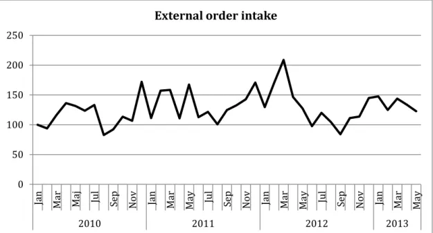
One of the key elements of this thesis was to investigate the possibilities of adding a quantitative time-series forecasting model to the current forecasting process at The Company. A number of different quantitative forecasting methods presented in the
29
academic literature on external order intake between January 2010 and May 2013 have been tested.
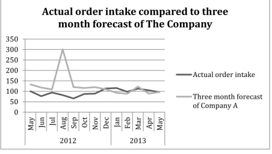
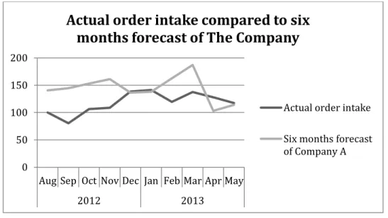
The test was constructed in such a way that historical data was applied to a quantitative model who forecasted value for time periods in the past. This way the forecast from the quantitative model can be compared to known actuals in the past. The test measured the accuracy on three and six months’ time frame, as those intervals was used among the staff at The Company. For a three months forecast, the first month that was forecasted differed depending on the model, but generally the first month forecasted was April 2010, and for a six months forecast the first forecast was usually made for July 2010. The accuracy of each forecast has then been evaluated through a number of different measures to see which performed the best. The quantitative forecasts have also been compared to the forecasts that TheCompany
has made between May 2012 and May 2013 in order to see whether they have any potential to increase the accuracy (there is no data available for forecasting accuracy made by The Company prior to May 2012).
3.5.1 Forecasting methods
Historical data was compiled in MS Excel in order to test the different models and to conclude which model that performed the best. The result of those tests, in combination with information gained through academic literature review and information from the interviews with employees, was the foundation of the discussion and final recommendation to The Company.
The models we chose to test were
3 Months Moving Average (3MA) 5 Months Moving Average (5MA)
Last Year Actual (LYA) (e g. Forecast for July 2011 is set as the actual value of July 2010)
Single Exponential Smoothing (SES)
Adaptive response rate single exponential smoothing (ARRESES) Holt’s method
Holt-Winter’s trend and seasonality measure Holt-Winter’s measure, trend excluded
All of these methods are well known within the field of business forecasting. They are presented in Makridakis et.al. (1998), and they were also used in the M-competitions (Makridakis & Hibon, 2000). The level of difficulty also varies among the different
30
methods, from simple methods such as MA and LYA, to more advanced methods such as Holt-Winter’s trend and seasonality measure.
A number of methods have of course been excluded from this report. The reason why they have been excluded is simply because they were too complex, and also not included in the work of Makridakis et. al. (1998). Examples of methods being deemed as too complex are the ARIMA-models. The guideline from the beginning was to come up with a forecasting method that would be simple to understand for The Company. ARIMA-methods need an understanding of autocorrelation and how to interpret data to change the model according to changes in the data. This is an understanding that The Company does not have in-house, thus it was excluded from the report.
As mentioned earlier in the report, the decision on which forecasting methods to construct and to test was made by the authors, the demand manager and the data intelligence managers in consensus. However, the authors had deeper understanding of different forecasting methods, and the process can be described as the authors presenting different forecasting methods to the demand manager and the data intelligence manager. During the presentation, it was explained how the method should be constructed, and how many variables it contained. The data manager and the demand