Testing Efficient Risk Sharing with Heterogeneous Risk Preferences:
Semi-parametric Tests with an Application to Village Economies
∗Maurizio Mazzocco and Shiv Saini University of Wisconsin-Madison
May 2006 Preliminary
Abstract
Previous tests of efficient risk sharing have assumed that households have identical risk preferences. This assumption is equivalent to the restriction that households can pool their resources, but cannot optimally allocate them according to individual risk preferences. In this paper, we first test the hypothesis of homogeneous risk preferences and reject it. This result implies that previous tests should have rejected efficiency even if households are perfectly sharing risk. We then derive two tests of efficient risk sharing that allow for heterogeneity in risk preferences. Using the two tests we cannot reject efficient risk sharing.
1
Introduction
Efficient risk sharing has been tested in several papers and it is generally rejected. Cochrane (1991), Mace (1991), Altonji, Hayashi, and Kotlikoff (1992), Townsend (1994), Hayashi, Altonji, and Kotlikoff (1996), Ravallion and Chaudhuri (1997), and Ogaki and Zhang (2001) are the main examples. These papers have two features in common. First, efficient risk sharing is tested using only variation in consumption expenditure. Second, it is assumed that households have identical preferences for risk.
∗We are very grateful to Pierre-Andr´e Chiappori, Mariacristina De Nardi, Dennis Kristensen, Rodolfo Manuelli,
Jack Porter, James Walker, and participants at seminars at UCLA, University of Western Ontario, and University of Wisconsin-Milwaukee and at the Conference on Macroeconomics of Imperfect Risk Sharing for helpful comments.
The assumption of homogeneous risk preferences imposes strong restrictions on the risk sharing test. To see this it is helpful to divide intra-household risk sharing into two parts. First, households pool their resources and consequently eliminate the idiosyncratic uncertainty that they are facing. We will refer to this component of risk sharing as income pooling. Second, households insure each other by allocating pooled income according to individual risk preferences. This component of risk sharing will be denoted by the term mutual insurance. A priori the mutual insurance component of risk sharing is at least as important as income pooling. The assumption of homogeneous risk preferences, however, is equivalent to the assumption that the optimal allocation of pooled resources is an insignificant fraction of risk sharing. If in the data this is not the case, a test of efficiency based on homogeneous risk preferences will reject efficiency even if households fully share risk.
This paper makes two main contributions. First, under efficiency we test if risk preferences are homogeneous across households and we reject this hypothesis. Second, we derive two tests of efficient risk sharing that allow for heterogeneous risk preferences. Using variation in consumption expenditure, we cannot reject efficient risk sharing.
The test of homogeneity in risk preferences is based on the following idea. Consider an economy characterized by efficient risk sharing with only two households. If risk preferences are heteroge-neous, the mutual insurance component of risk sharing must be a feature of household behavior. Mutual insurance implies that for some realizations of pooled income household 1’s consumption will be larger than household 2’s, whereas for other realizations household 2 will consume more. As a consequence, household 1’s consumption as a function of aggregate resources will cross the con-sumption function of household 2. Thus, under efficiency if the concon-sumption functions of households 1 and 2 cross, the hypothesis of homogeneous risk preferences is rejected. Using the International Crops Research Institute for the Semi-Arid Tropics (ICRISAT) data on non-durable consumption, leisure, and wages we find strong evidence against the hypothesis that households have identi-cal preferences for risk. This result has two implications. First, previous papers that have used ICRISAT should have rejected efficiency even if households share risk efficiently. Second, any test of efficiency should allow for heterogeneity in risk preferences.
The two tests of efficiency that we propose are based on the following result. We show that if households share risk efficiently, their consumption must be an increasing function of pooled resources. We also show that this restriction is the only testable implication of efficient risk sharing if (i) the only assumptions on the household utility functions are non-satiation and concavity and
(ii) only longitudinal variation in consumption is observed. Any other testable implication is the result of additional assumptions on household preferences. This result contains two testable impli-cations. First, household consumption should increase with pooled resources. Second, household consumption should be a function of pooled income in the sense that for any realization of pooled resources one should never observe two different levels of household consumption. This implies that after controlling for pooled resources, household consumption should not dependent on variables that capture idiosyncratic shocks. We test both implications by allowing for heterogeneous risk preferences.
This paper is one of the first attempts to test efficient risk sharing using the restriction that household consumption should increase with pooled resources. The main advantage of this test is that it does not require the choice of alternative variables, which is sometimes arbitrary and affected by endogeneity in case of nonseparability between consumption and leisure. This implication of efficiency is first tested under the assumption that consumption and leisure are separable. We reject efficient risk sharing in 8 out of 1122 possible cases. We then test the restriction allowing for non-separability between consumption and leisure. In this case we reject the hypothesis that households share risk efficiently in only one case.
The second implication tested in this paper is the standard restriction tested in the efficiency literature. Our test, however, differs from previous ones in two respects. First, households can have different preferences for risk. Second, we use a semi-parametric approach to estimate consumption as a function of pooled resources and other variables. Consequently the choice of the functional form for the consumption functions has smaller effects on the outcome of the tests. The test is implemented using non-labor income as an additional variable first under the assumption of separability between consumption and leisure and then without this assumption. In both cases we cannot reject the hypothesis that non-labor income does not affect household expenditure. This indicates that if risk preferences are allowed to vary across households, there is little or no evidence against efficient risk sharing.1
The paper proceeds as follows. In section 2 we discuss the tests proposed in previous papers. In section 3, we present a model of efficient risk sharing. In section 4, we derive the testable
1Schulhofer-Wohl (2006) also tests efficient risk sharing allowing for heterogeneity in risk preferences. The paper differs in several respects from ours. First, there is no test of heterogeneity in risk preferences. Second, the author uses only the test previously used in the risk sharing literature. Third, the standard risk sharing test is implemented using the PSID.
implications of homogeneity in risk preferences and efficiency. In section 5, the data used in the tests are described. In section 6, we discuss the semi-parametric estimation of the household expenditure function and its derivatives. Section 7 presents the results under the assumption that preferences are separable between consumption and leisure. Section 8 reports the results with non-separable preferences. Section 9 concludes.
2
Tests of Efficient Risk Sharing in the Literature
In this section we discuss the tests of efficiency used in the risk sharing literature. Consider an economy in which the households have different preferences, are endowed with risky incomes, and can share risk efficiently among them. The allocation of risk in this economy can be divided into its income pooling and mutual insurance components. Several papers have tested whether households share risk efficiently in this type of economy. The main examples are Cochrane (1991), Mace (1991), Altonji, Hayashi, and Kotlikoff (1992), Townsend (1994), Hayashi, Altonji, and Kotlikoff (1996), Ravallion and Chaudhuri (1997), and Ogaki and Zhang (2001). The tests used in those papers are valid tests of efficient risk sharing only if mutual insurance is an insignificant part of risk sharing.
To see this consider the following simple example. The example and the related discussion is not meant to diminish the importance of the papers mentioned above. Those paper had and are still having a significant influence in economics that goes beyond the efficiency test. The discussion is meant to point out a crucial deficiency in the proposed tests. The economy is composed of two households living for T periods in an environment with uncertainty. As it is standard in this literature, it is assumed that preferences are separable over time, across states of nature, and between consumption and leisure.2 Each household is characterized by preferences that belong to the Harmonic Absolute Risk Aversion (HARA) class, i.e. ui
c(c) = (ai+c)−γi. The HARA class
includes the most commonly used utility functions, namely the Constant Absolute Risk Aversion (CARA) and the Constant Relative Risk Aversion (CRRA) utility functions.
A necessary and sufficient condition for efficient risk sharing is that the ratio of marginal utilities is constant across states of nature and over time and equal to the ratio of Pareto weights. This
2Hayashi, Altonji, and Kotlikoff (1996) use preferences that are nonseparable in consumption and leisure. The intuition provided in this section applies also to those papers. However, a model with nonseparable preferences allows for more general patters of household consumption. We consider this more general case in the next sections.
implies that for each periodt and for each stateω, µ1u1c ¡ c1t,ω¢=µ2u2c ¡ c2t,ω¢, (1)
where household consumptionc1
t,ω and c2t,ω must satisfy the resource constraint
c1t,ω+c2t,ω =Yt,ω,
withYt,ω equal to pooled resources in periodt and stateω.
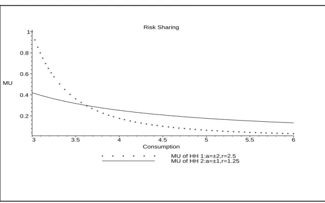
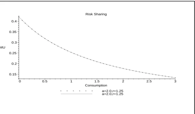
Figure 1 depicts the efficiency condition (1) for different realization ofYt,ω and for the following set of preference parameters: a1= 1,a2 = 2,γ1 = 2.5,γ2= 1.25,µ1 =µ2. This figure can be used to describe the efficient allocation of risk between household 1 and 2. In the example considered here,µ1u1c and µ2u2c cross once. It can be shown that under the assumption of HARA preferences
these two functions can cross zero, one, or two times. We analyze the one-crossing case because it also provides the insight for the zero-crossing and the two-crossings case. Figure 1 is characterized by two regions. The region on the left of the crossing corresponds to adverse realizations of pooled resources. Here the less risk averse household consumes less than half of pooled resources. This allocation of aggregate income can be interpreted as the outcome of the insurance provided by the less risk averse household against adverse realizations. The second region is characterized by good realizations. Here the less risk averse household consumes more than half of pooled resources as a compensation for the insurance provided. The main implication of all this is that the less risk averse household has more volatile consumption paths.
Consider now the same economy except that the two households have identical HARA prefer-ences. This example encompasses the cases considered by Cochrane (1991), Mace (1991), Altonji, Hayashi, and Kotlikoff (1992), Townsend (1994), Ravallion and Chaudhuri (1997), and Ogaki and Zhang (2001).3 Figure 2 depicts the corresponding efficiency condition under the assumption that
3Townsend (1994) reports two sets of results. One set is obtained using the panel of households interviewed by the International Crops Research Institute of the Semi-Arid Tropics (ICRISAT). In this case, it is assumed that all households have identical CARA preferences. The second set of results is obtained by regressing changes in individual consumption on changes in aggregate resources and individual income for each household separately using six or ten observations at a time. In this case, households are characterized by heterogeneous CARA preferences. Note that CARA utility functions are obtained as the limit of a HARA utility function as the curvature parameterγ tends to infinity. Consequently, heterogeneous CARA preferences allow for different subsistence levelsai, but the curvature
parameter cannot differ across households. Using this result it can be shown that this class of preferences does not allow for the mutual insurance component of risk sharing. However it is true that with heterogeneous CARA
the two households have identical Pareto weights. In this case, the two households consumes half of pooled resources for each realization ofYt,ω. Figure 3 describes the same economy except that
µ1 > µ2. In this case the household with higher Pareto weight always receives a larger fraction of aggregate resources. The assumption of identical preferences is therefore equivalent to assuming that in the economy there is no mutual insurance.
To understand the effect of ignoring mutual insurance on the tests used in previous papers, we consider a generalization of the test employed in Mace (1991). The generalization allows for any utility function that belongs to the HARA class as long as households have identical prefer-ences. Consequently, it includes as special cases the tests used in Cochrane (1991), Mace (1991), Altonji, Hayashi, and Kotlikoff (1992), Townsend (1994), Ravallion and Chaudhuri (1997), and Ogaki and Zhang (2001). To simplify the discussion, it is assumed that the there is no observable or unobservable heterogeneity. The generalization of Mace’s test can be written in the following form:4 f¡cit+1¢−f¡cit¢= 1 J J X j=1 ³ f ³ cjt+1 ´ −f ³ cjt ´´ .
wheref(c) =cfor CARA preferences,f(c) = log (c) for CRRA preferences, andf(c) = log (a+c) for HARA preferences and J is the number of households in the economy. According to this equation, under efficiency the first difference of transformed household consumption should be equal to the first difference of aggregate transformed consumption. This implies that the first difference of householdi’s transformed consumption must equal the first difference for every other household in the economy. For instance, for CRRA preferences the consumption growth of householdishould equal consumption growth of every other household in each periodt and stateω.
Now consider an economy in which households have the heterogenous HARA preferences used in figure 1. Suppose that in period t the economy is characterized by an adverse realization of aggregate resources. According to figure 1, in this period the economy is characterized byc2
t < c1t.
Suppose that att+ 1 a good realization of resources prevails. In this case c1t < c2t. This implies that f¡c1t+1¢−f¡c1t¢< 1 2 2 X j=1 ³ f ³ cjt+1 ´ −f ³ cjt ´´ < f¡c2t+1¢−f¡c2t¢,
which contradicts the test used in Mace (1991) and in the other papers.5
preferences the weighted marginal utilities may cross if there is heterogeneity in Pareto weights. But this is only a consequence of different Pareto weights and not of heterogeneity in risk preferences.
4The dependence on the state of nature is suppressed for ease of exposition.
To summarize the assumption of identical preferences is equivalent to the assumption that there is no mutual insurance component of risk sharing, and that one should only focus on income pooling. If in the economies studied in the risk sharing literature risk preferences are heterogeneous and mutual insurance is a significant part of risk sharing, previous papers should have rejected efficiency even if household behavior is fully efficient.
The previous discussion suggests that efficient risk sharing may have been rejected in the past because mutual insurance was not considered. Observe, however, that in previous papers efficient risk sharing was rejected by testing whether changes in individual consumption are explained by changes in individual income even after controlling for changes in aggregate consumption. In the risk sharing literature the coefficient on income is generally statistically significant and positive.6 Can the failure to consider mutual insurance explain this result? The answer to this question is positive if households with lower risk aversion have more volatile income processes.7
To see this note that with heterogeneous preferences household consumption is a household-specific function of aggregate resources. Under HARA preferences the differences in utility func-tions can be summarized by the heterogeneity in curvature parameterγi and subsistence level ai.
Household consumption can therefore be written in the following form:
fi¡cit+1¢=g¡Cta+1, ai, γi
¢ .
wherefi(c) is the function introduced earlier in this section. A first order Taylor expansion around
the averageγi in the economy implies that the consumption function can be written as follows:
fi¡cit+1¢'g¡Cta+1, ai,γ¯ ¢ + (γi−¯γ) ∂γ∂ ig ¡ Cta+1, ai, γi ¢¯¯ ¯ ¯ ¯ γ .
The first difference in household consumption can therefore be written in the following form:
∆fi¡cit+1¢'∆g¡Cta+1, ai,¯γ ¢ + (γi−¯γ) ∂γ∂ i∆g ¡ Cta+1, γi, ai ¢¯¯ ¯ ¯ ¯ γ . (2)
preferences enables one to include in the constant the terms that capture aggregate quantities, 1
γj
logµt+1
µt
in equation (8) in Cochrane (1991). If preferences are heterogeneous these terms become household specific and they are equivalent to a household fixed effect in a panel estimation. Since the main idea in Cochrane (1991) is to use cross-sectional data instead of panel data, it is not possible to control for the household fixed effect. Consequently, Cochrane’s and Mace’s tests are affected by the same problem.
6Ogaki and Zhang (2001) find that the coefficient is positive and significantly different from zero in the ICRISAT for Aurepalle when they allow for a subsistence level and for Shirapur when they set the subsistence level to zero.
Figure 1 indicates that, if the households in this economy have differentγi, ∆fi¡ci t+1
¢
is a decreasing function of γi. Hence, the second term on the right hand side of (2) is positive for the less risk
averse households and negative for the more risk averse households. The efficiency test is generally performed by estimating the following equation:
∆fi¡cit+1¢−∆g¡Cta+1, ai,γ¯¢=α+ξ∆yit+1+²it+1.
for some functions fi(.) andg(.). If the economy is composed of households with heterogeneous
curvature parametersγi that share risk efficiently, the error term²i
t+1 has the following form:
²it+1=−ξ∆yti+1+ (γi−γ¯) ∂γ∂ i∆g ¡ Cta+1, γi, ai ¢¯¯ ¯ ¯ ¯ γ +ηit+1, where E¡ηi t+1|∆yt+1 ¢
= 0. Using the equation defining the error term, the OLS estimate of the income coefficient can be computed as follows:
ˆ ξ = Pn i=1 PT t=1 Ã (γi−γ¯) ∂γ∂ i∆g(C a t, γi, ai) ¯ ¯ ¯ ¯ ¯ γ +ηi t+1 ! ∆yi t+1 Pn i=1 PT t=1 ¡ ∆yi t+1 ¢2
wherey denotes demeaned income. This implies that asymptotically,
E ³ ˆ ξ ´ =V AR¡∆yti+1¢−1Cov à ∆yit+1, (γi−¯γ) ∂γ∂ i ∆g¡Cta+1, γi, ai ¢¯¯ ¯ ¯ ¯ γ ! .
Under the assumption that less risk averse households have more volatile income processes,
Cov à ∆yit+1, (γi−γ¯) ∂γ∂ i∆g(C a t, ai, γi) ¯ ¯ ¯ ¯ ¯ γ ! >0,
which implies that the coefficient on individual income will be on average positive as it was found in previous papers.
Theoretically the failure of considering heterogeneous risk preferences and mutual insurance can explain the rejection of efficiency. Are heterogeneous risk preferences and mutual insurance important features of risk sharing in the data? The rest of the paper is devoted to answering this question by developing tests that allow for risk preferences that vary across households.
3
A Model of Efficient Risk Sharing
In this section we describe the model of efficient risk sharing that will be used to derive the tests. Consider an economy in which households live for τ periods. In each period t, let ωt denote the
realization of all variables in the economy. For a given history of realizations ht = (ω1, ..., ωt), in period t household i is endowed with a wage wi
t(ht) and a total amount of time Tti(ht) that
can be divided between leisure and labor. The aggregate amount of non-labor resources in the economy is denoted byYt(ht), where Yt(ht) may include profits and saving. Letcit(ht) and lit(ht)
be, respectively, consumption and leisure of householdiin period t conditional on the history ht.
Household preferences are assumed to be separable over time and across states of nature. They are allowed to depend on observable and unobservable heterogeneity, which will be denoted by
zi
t(ht) andηti(ht). The corresponding utility functionui
£ ci
t(ht), lit(ht) ;zti(ht), ηit(ht)
¤
is assumed to be strictly increasing, strictly concave, and twice continuously differentiable in consumption and leisure. Households are characterized by a common discount factor β and share the same beliefs over histories of realizations, which are denoted byP(ht).
Efficient risk sharing in this economy can be described using a standard Pareto problem. Let
µi be the Pareto weight assigned to householdi with
Pn
i µi = 1 and suppose for simplicity that
0< µi <1. The efficient allocation of resources is then the solution of the following problem:
max {ci t(ht),lit(ht)} n X i=1 µi τ X t=1 βtX ht P(ht)ui £ cit(ht), lit(ht) ;zti(ht), ηti(ht) ¤ (3) s.t. n X i=1 ¡ cit(ht) +wit(ht)lit(ht) ¢ =Yt(ht) + n X i=1 wti(ht)Tti(ht) for each t,ht, cit(ht)>0, 0≤lit(ht)≤Tti(ht) for eacht,ht,
where the right hand side of the resource constraint is full income in the economy.8
The solution of the Pareto problem (3) can be characterized using three stages. The decom-position of the problem in stages will be helpful in dealing with observable and unobservable heterogeneity in the tests. In the last stage, let ρi
t(ht) be an arbitrary amount of aggregate
re-sources allocated to householdi. Then in each periodtand for each history ht, householdichoose consumption and leisure by solving the following individual problem:
Vi¡ρit(ht) ;wti(ht), zit(ht), ηit(ht) ¢ = max ci t(ht),lit(ht) ui£cit(ht), lit(ht) ;zit(ht), ηit(ht) ¤ (4) s.t. cit(ht) +wit(ht)lti(ht) =ρit(ht) cit(ht)≥0, 0≤lti(ht)≤Tti(ht).
8We model Pareto efficiency using full income because in small economies, for instance in villages, wages are imposed from the outside and are not the outcome of an equilibrium in the economy.
In the second stage, letρi,jt (ht) denote the amount of aggregate resources allocated to household
iand j. In each periodtand for each historyht, householdiand jthen choose the optimalρit(ht)
andρjt(ht) as the solution of the following problem:9
Vi,j ³ ρi,jt ;wti, wjt, zit, ztj, ηti, ηtj ´ = max ρi t,ρ j t µiVi ¡ ρit;wti, zti, ηit¢+µjVj ³ ρjt;wjt, zjt, ηtj ´ (5) s.t. ρit+ρjt =ρi,jt .
Observe that the solution of this problem is only a function of wages and heterogeneity of households
iandj, i.e. ρkt =ρkt ³ ρti,j;wti, wjt, zti, ztj, ηit, ηjt ´ fork=i, j.
This result and this stage are important for the derivation of the tests because, after accounting for
ρi,jt , they will enable us to control for the wages and heterogeneity variables of only two households. Without this stage one would have to control for the wages and heterogeneity variables of all the households in the economy.
In the first stage, aggregate resources available in period t conditional on the history ht are
allocated to each pair of households by solving the following problem:10
V Ã Yt+ n X i=1 witTti;wt, zt, ηt ! = max {ρ2ti−1,2i} n/2 X i=1 V2i−1,2i ³ ρ2ti−1,2i;w2ti−1, w2ti, zt2i−1, z2ti, ηt2i−1, η2ti ´ s.t. n/2 X i=1 ρ2ti−1,2i =Yt+ n X i=1 witTti,
wherewt,zt, and ηt are the vectors of wages and heterogeneity variables.
Under the standard assumptions that preferences are separable over time, across states of nature, and that consumption and leisure of household i are separable from consumption and
9Unless required for expositional clarity, the dependence on the history of realizations will be suppressed in the rest of the paper.
10The Pareto problem can be decomposed in three stages by pairing households in different ways. Here we consider one possible set of pairs under the assumption that there is an even number of households in the economy. Ifn is odd, three households will have to be arranged in one group.
leisure of every other household, it follows that τ X t=1 βtX ht P(ht)V Ã Yt(ht) + n X i=1 wit(ht)Tti(ht) ;wt(ht), zt(ht), ηt(ht) ! = max {ci t(ht),lit(ht)} n X i=1 µi τ X t=1 βtX ht P(ht)ui£cit(ht), lit(ht) ;zti(ht), ηti(ht)¤ s.t. n X i=1 ¡ cit(ht) +wit(ht)lit(ht) ¢ =Yt(ht) + n X i=1 wti(ht)Tti(ht) for each t,ht, cit(ht)≥0, 0≤lit(ht)≤Tti(ht) for eacht,ht,
i.e. the solution of the three-stage problem is equivalent to the original Pareto problem. To provide the intuition underlying this result note that under the assumptions made in this paper, the conditions of the second welfare theorem are fulfilled. As a result the solution of the Pareto problem can be decentralized using transfers.
4
Testable Implications
In this section we derive testable implications of homogeneity in risk preferences and efficient risk-sharing using the second stage of the efficiency problem described in the previous section. The discussion will be divided into two parts. In the first part we will consider an economy where households share risk efficiently and we will derive a restriction that will enable us to test whether risk preferences are homogeneous across households. In the second part of this section we will consider two possible environments. In the first environment, household preferences are separable between consumption and leisure. In the second environment, household preferences are non-separable but for each household there is no variation in real wages across states of nature and over time. We will find necessary and sufficient conditions for efficient risk sharing and show that they are identical in these two environments. To simplify the discussion, we will assume throughout the section that there is no observable or unobservable heterogeneity.
Consider an economy where households share risk efficiently. The testable restriction of homo-geneity in risk preferences is based on the following idea. Suppose that household i and j fully insure each other. As discussed in section 2, if for some realizations of total income householdi
receives a larger amount of pooled resources and for other realizations householdj receives a larger amount, their marginal utilities must cross. If their marginal utilities cross their risk preferences cannot be identical. Consequently, under efficiency if in one periodρi > ρj and in a different period
ρi < ρj, the two households cannot have identical preferences for risk. This idea is formalized in
the following propositions.
Proposition 1 Suppose that householdiandj share risk efficiently. If there exist two realizations
of total incomeρi,j and ρ¯i,j such that
ρi¡ρi,j, wi, wj¢> ρj¡ρi,j, wi, wj¢ and
ρi¡ρ¯i,j, wi, wj¢< ρj¡ρ¯i,j, wi, wj¢,
householdi and household j cannot have identical risk preferences.
Proof. In the appendix.
We will now derive testable implications of efficient risk sharing. Consider an economy where either household preferences are separable between consumption and leisure or real wages can vary across households but for each household they are constant for eachω and for eacht. This is the case considered in previous papers that have tested efficient risk sharing. Mace (1991), Townsend (1994), Altonji et al. (1992), Ravallion and Chaudhuri (1997), and Ogaki and Zhang (2001) assume separability between consumption and leisure. Cochrane (1991) uses a cross-section of households and hence ignores any longitudinal variation in real wages. Hayashi et al. (1996) exploit longitudinal consumption variation after controlling for longitudinal variation in leisure. This is equivalent to using longitudinal variation in consumption after having removed the portion that is explained by longitudinal variation in real wages.
To derive testable implications in this economy, consider households iand j and observe that under efficiency the following two restrictions must be fulfilled. First, after controlling for differences in real wages across households, only pooled income should affect the amount of resources received by the householdsiandj. Hence, for eachρi,j only one value should be observed forρi¡ρi,j, wi, wj¢
andρj¡ρi,j, wi, wj¢. Second, an increase in pooled income should increase the amount of resources
allocated to household i as well as to household j. If one of these restrictions is not satisfied, household behavior is not only affected by changes in pooled income as predicted by efficient risk sharing, but also by idiosyncratic shocks. These two restrictions imply that a necessary condition for efficient risk sharing is thatρi¡ρi,j, wi, wj¢ and ρj¡ρi,j, wi, wj¢are strictly increasing functions of
and concave household utility functions this condition is also sufficient in the following sense. If
ρi¡ρi,j, wi, wj¢andρj¡ρi,j, wi, wj¢are strictly increasing functions ofρi,j, then it is always possible
to find increasing and concave household utility functions and Pareto weights such that efficiency is satisfied. All this implies that if only variation in expenditure is observed, the only testable implication of efficient risk sharing is that the amount of resources allocated to each household are an increasing function of total income. Any other restriction is the outcome of the particular function form selected for household preferences. The following proposition summarizes this result.
Proposition 2 Suppose that the utility functions of household iand j are strictly increasing and
concave. Then, if householdsi and j share risk efficiently,ρi¡ρi,j, wi, wj¢and ρj¡ρi,j, wj, wi¢are
strictly increasing functions of pooled income.
Suppose in addition that preferences are separable between consumption and leisure or wi and
wj are constant. Then, if ρi¡ρi,j, wi, wj¢ and ρj¡ρi,j, wj, wi¢ are strictly increasing functions of
pooled income, there exist utility functions that are strictly increasing and concave such that the two households share risk efficiently.
Proof. In the appendix.
In the remaining sections the results presented here will be used to evaluate whether households in Indian villages share risk efficiently.
5
Estimation of the Expenditure Functions
The tests proposed in this paper require a separate estimate of the expenditure functionρk¡ρi,j, wi, wj;zi, zj, ηi, ηj¢
for each household. With heterogeneous risk preferences, there is no close form solution for the household expenditure function. This implies that a parametric approach would have to rely on approximations of this function.11 To avoid this problem, a semi-parametric approach is used in the estimation. In the rest of the paper we will use the term observable and unobservable heterogeneity to refer to differences inz and η across households, and we will use the term heterogeneity in risk preferences to refer to differences across household utility functions.
The semi-parametric estimator of the expenditure functions used here requires four assump-tions. First, we will assume that observable and unobservable heterogeneity enter the expenditure
11A close form solution exists for heterogeneous CARA preferences. However, all CARA preferences have identical curvature parameters and therefore no heterogeneity in the only feature of risk preferences that is crucial for the insurance component of risk sharing.
functions only as a linear combination of the difference betweenzi andzj, and ηi andηj, i.e. only
di,j =θ i,j
¡
zi−zj¢+ηi−ηj affectsρk. This assumption simplifies significantly the estimation since
all the variation in heterogeneity is captured by the single index di,j. Second, it is assumed that
the unobservable component of heterogeneity does not change over time. Under this assumption, the effect ofηi−ηj can be captured by adding a constant to the vector of observables z.12 As a third assumption, to reduce the variance of the estimates we will impose the restriction that the coefficients on the observable heterogeneity terms are common across households. Lastly, in the estimation we allow for measurement errorsm that are additive in individual expenditure. Under these assumptions, the expenditure function of householdk can be written in the form,
ρkt =gk ³ ρi,jt , wti, wjt, di,jt ´ +mkt, (6) wheredi,jt =θ ³ zi t−ztj ´
+ηi−ηj. Since total expenditureρi,j
t is the sum of individual expenditures,
ρi,jt depends on the error term mk. In the estimation we will consider this dependence using an estimator that allows for endogenous variables. But we will assume that mk is independent of
wages and heterogeneity variables.
There is a large class of preferences that generates the expenditure function (6). For instance, all the utility functions that can be written in the following form belong to that class:
ui¡ci, li, zi, ηi¢=v¡ci, li¢exp¡θzi+ηi¢. (7)
The expenditure functions are estimated as follows. Suppose that the parameters θ on the heterogeneity variables are known. The functiongkcan then be estimated using standard
nonpara-metric methods. To take into account that in general E h mk|ρi,j t , wit, wtj, di,j i = E h mk|ρi,j t i 6 = 0, we use the nonparametric approach developed by Newey, Powell, and Vella (1999). We will briefly describe the method.
Letq be a set of instruments in the sense that the following conditions are satisfied:13
ρi,j =h¡qi,j¢+ui,j, E£ui,j|qi,j¤= 0, and E h mk|ui,j, qi,j i =E h mk|ui,j i .
For a linear functionh, the moment conditions are equivalent to the assumption thatqis orthogonal
12It is straightforward to modify the estimator used in this paper to allow ηi−ηj to vary over time. In this case
we can follow Blundell and Powell (2001) and consider the expectation of the expenditure function overηi−ηj. This
approach, however, requires a larger panel than the one that is available to us.
touand mk. Then, we have that
E h
ρk|ρi,j, wi, wj, di,j, qi,j i
=gk¡ρi,j, wi, wj, di,j¢+E h
mk|ρi,j, wi, wj, di,j, qi,j i
=gk¡ρi,j, wi, wj, di,j¢+E h
mk|ui,j, qi,j i
=gk¡ρi,j, wi, wj, di,j¢+λ¡ui,j¢,
whereλ(u) =E£mk|u¤. Newey et al. (1999) propose to estimate the functiongk in two steps. In
the first step the error termu is estimated nonparametrically as ˆui,j =ρi,j−ˆh¡qi,j¢. In the second
step, the additive regression
ρk=gk¡ρi,j, wi, wj, di,j¢+λ¡ui,j¢+²k, (8)
is estimated using the estimated residuals ˆuin place of the true ones. An estimator of the function
gk can then be recover by isolating the components that do not depend on the residuals u. In
this paper, all the nonparametric estimations are performs using the series estimator suggested by Newey et al. (1999) with polynomials.
The parameters on the heterogeneity variables are not known, but they can be estimated using one of the semi-parametric methods developed for the estimation of single-index models. In this paper we use the semi-parametric least square approach proposed by Ichimura (1993).
6
The Tests
The next three subsections describe the approach used to test homogeneity in risk preferences and efficiency.
6.1 Test of Homogeneous Risk Preferences
The test of homogeneity in risk preferences is based on the result that under efficiency and identical risk preferences the expenditure functions should not cross. We are unaware of any test in the econometric or statistical literature that enables one to test whether two functions cross. For this reason we construct a new test which is based on the following idea.
Consider the difference between householdi’s and household j’s expenditure functions:
ρi−ρj =gi¡ρi,j, wi, wj, di,j¢−gi¡ρi,j, wi, wj, di,j¢+mi,j =gi,j¡ρi,j, wi, wj, di,j¢+mi,j.
For any given realization of wi, wj, di,j, under identical risk preferences gi,j as a function of
maximum of gi,j¡ρi,j¢ multiplied by its minimum should always be positive. Consequently, if
max©gi,jªmin©gi,jªis negative the null is rejected and the two households must have
heteroge-neous preferences.
The test is constructed in two steps using the previous idea. We first estimate the function
gi,j using the method described in the previous section and the corresponding variance using the
estimator proposed by Newey et al. (1999). Denote by ˆgi,j and V AR¡gˆi,j¢the estimates and let
¯ gi,j¡ρi,j¢= gˆ i,j¡ρi,j¢ r V AR ³ ˆ gi,j³ρi,j t ´´,
where we divide by the standard error so that ˆgi,j has the same variance for each ρi,j. The test
statistic is then defined as
ˆ
ξ1 = max ©
¯
gi,jªmin©g¯i,jª.
In the second step, we bootstrap the distribution of ˆξ1 and we reject the null if ˆξ1 is too small, i.e. if ˆ ξ1 s ³ ˆ ξ1 ´ < q∗(0.05), wheres ³ ˆ ξ1 ´
is the standard error of ˆξ1 and q∗(0.05) is the 5-th percentile of the empirical distri-bution.
Two remarks should be discussed. First, we divide ˆgi,j by its standard error to increase the
power of the test. To understand why this transformation increases the power of the test, suppose that we use ˆgi,j instead of ¯gi,j and consider ˆgi,j at four different levels of total expenditure: ρi,j
1 ,
ρi,j2 ,ρi,j3 , and ρi,j4 . Assume that
ˆ
gi,j ³
ρi,j1 ´
= max©gˆi,jª>gˆi,j
³ ρi,j2 ´ >0, and ˆ gi,j ³ ρi,j3 ´
= min©ˆgi,jª<ˆgi,j ³
ρi,j4 ´
<0.
Suppose also that the variance of ˆgi,jatρi,j
1 andρi,j3 is so large that the function at these two points is not statistically different from zero. But the variance at ρi,j2 and ρi,j4 is small enough that ˆgi,j
is statistically positive in the first case and negative in the second case. Then the test would not reject the null even if the alternative is correct. By dividing by the standard error we avoid this problem because ¯gi,j has the same variance at each point.
As a second remark, note that the 5-th percentile can be computed using different methods. Hall (1992) and Horowitz (2002) argue that the percentile-t bootstrap method have better theoretical properties than the standard percentile method. For this reason we follow Hall (1992) and Horowitz (2002) and computeq∗(0.05) as follows. For each bootstrap we compute the bootstrap t-statistics
ˆ ξ∗ 1−ξˆ1 s ³ ˆ ξ∗ 1 ´, where ˆξ∗ 1 and s ³ ˆ ξ∗ 1 ´
are computed using the bootstrap sample and ˆξ∗
1 using the original sample. The 5-th percentile is then calculated using the bootstrap t-statistics.
6.2 Test of Efficiency with Excluded Variables
The first test of efficiency that we perform is the standard test of excluded variables: after control-ling for total expenditure, wages, and heterogeneity, any variable that captures household specific shocks should not enter the expenditure function. The main difference between the test used here and previous tests is that we employ a semi-parametric approach to allow for differences in risk preferences.
The semi-parametric approach is based on the test proposed by Fan and Li (1996). Suppose that the expenditure function of householdidepends on an excluded variableyi. Then the function can be written in the following form:
ρi =gi¡ρi,j, wi, wj, di,j, yi¢+λ¡ui,j¢+²i=fi¡Xi,j, yi¢+²i,
where Xi,j contains ρi,j, wi, wj, di,j, and ui,j, and E£²i|Xi,j, yi¤ = 0. Under the null
hypoth-esis of efficiency fi¡Xi,j, yi¢ = E£ρi|Xi,j, yi¤ = E£ρi|Xi,j¤ = ri¡Xi,j¢, but under the alter-native fi¡Xi,j, yi¢ 6= ri¡Xi,j¢. Let u = ρi −ri¡Xi,j¢. Then, E£ui|Xi,j, yi¤ = fi¡Xi,j, yi¢−
ri¡Xi,j¢ = 0 under the null and E£ui|Xi,j, yi¤ 6= 0 under the alternative. All this implies that
E£uiE£ui|Xi,j, yi¤¤=Eh©E£ui|Xi,j, yi¤ª2i≥0, where the equality holds if and only if the null
hypothesis is correct. Fan an Li propose as a test statistic a sample analog ofEh©E£ui|Xi,j¤ª2i,
with the residuals u being replaced by estimated ones. The proposed sample analog has the fol-lowing form: 1 n X i £ uifX ¤
E£uif¡Xi,j¢|Xi,j, yi¤f¡Xi,j, yi¢,
In this paper we estimate the residuals using the series estimator described in section 5. The densities and the conditional expectation are estimated using a standard kernel estimator. The distribution of the test statistic ˆξ2 is obtained using bootstrap. The null hypothesis is then rejected if ˆξ2 is too large, i.e. if
ˆ ξ2 s ³ ˆ ξ2 ´ > q∗(0.95),
whereq∗(0.95) is the 95-th percentile obtained using the percentile-t bootstrap method. The test will be performed using non-labor income as the excluded variable.
6.3 Test of Efficiency with Increasing Expenditure Functions
The second test of efficiency evaluates whether the household expenditure function is increasing in total resources and rejects efficient risk sharing if part of the function decreases withρi,j. The
test that we use in this paper is a generalization of the monotonicity test introduced by Hall and Heckman (2000) to a model with multiple regressors and endogeneity.
The intuition underlying the test can be described a follows. Consider householdi’s expenditure as a function only ofρi,j and suppose that there is no endogeneity issue. Then,
ρi =g ¡ ρi,j¢+². (9) Let n³ ρi t, ρi,jt ´ ,1≤t≤T o
be data generated by equations (9) and denote by
n³ ¯ ρi t,ρ¯i,jt ´ ,1≤t≤T o
the same data sorted in increasing order of total expenditureρi,j. Consider a subset of the sorted
data n³ ¯ ρi t,ρ¯i,jt ´ , r≤t≤s o
and estimate the slope of a linear regression ofρi on ρi,j. Repeat the
last step for any subset of the sorted data that contains enough information to estimate the slope. Hall and Heckman’s idea is that under the hypothesis that the function g¡ρi,j¢ is increasing, the
minimum over all the estimated slopes should not be negative.
Formally the test statistic is defined as follows. For a given integermthat will be defined later, letr and sbe integers that satisfy 0≤r ≤s−m ≤T −m and let aand b be scalars. Denote by
h¡wi, wj, di,j¢a polynomial in the wages and in the heterogeneity term and byδ¡ui¢a polynomial
in the endogeneity residuals. Define
S(a, b, h, δ|r, s) = s X i=r+1 © ρi−£a+bρi,j+h¡wi, wj, di,j¢+δ¡ui¢¤ª.
least square problem: ³ ˆ a,ˆb,ˆh,ˆλ ´ =argmin S(a, b, h, λ|r, s).
The integerm must therefore be larger than the sum of the order of the polynomials plus 2. The variance matrix of the estimated coefficients is equal to σ2(X0X)−1, where σ2 is the variance of the residuals²of the expenditure equation (8) andX is the matrix of regressors. This implies that the variance of q ˆb
(X0X)−1
b,b
is equal to σ2 where (X0X)−1
b,b is the diagonal element of the inverse
matrix that corresponds to ˆb. The test statistic can then be defined as
ˆ ξ3 = max − ˆb(r, s) q (X0X)−1 b,b : 0≤r ≤s−m≤T−m .
The test rejects the null if ˆξ3 is too large. Note that the integer m plays the role of a smoothing parameter in the sense that larger values ofm reduce the effect of outliers.
The distribution of the test statistic is derived using the bootstrap method suggested by Hall and Heckman (2000). Note that the most difficult nondecreasing function for which to test is a function that is constant inρi,j. Thus, the distribution of ˆξ
3 is obtained under the hypothesis that the function being tested has this feature. In this case we have that
ρi=gi¡k, wi, wj, di,j¢+²i,
for some constant k. Note that λ(u) is not included because for a constant ρi,j there is no en-dogeneity issue. The distribution of the test statistic should then be computed by replacing the previous definition ofS(a, b, h, λ|r, s) with
S(a, b, h, λ|r, s) =
s
X
i=r+1 ©
gi¡k, wi, wj, di,j¢+²i−£a+bρi,j+h¡wi, wj, di,j¢+δ¡ui¢¤ª. (10)
The distribution of ˆξ3 can therefore be derived in three steps. First, for each bootstrap sample we estimate the residuals ²i and the function gi¡k, wi, wj, di,j, yi¢ using the method discussed in section 5. In the second step, we estimate ˆξ3 using the bootstrap sample and (10). In the final step we compute the 95-th percentile of the distribution of ˆξ3 and reject the null if
ˆ ξ3 s ³ ˆ ξ3 ´ > q∗(0.95),
One remark is in order. In the derivation of the distribution of ˆξ3 the order of the polyno-mial h¡wi, wj, di,j¢ is set equal to the order used in the estimation of gi¡k, wi, wj, di,j¢.
Other-wise the choice of the constant for k affects the least square estimate of the coefficient on ρi,j in
S(a, b, h, λ|r, s).
7
Data and Econometric Issues
In the next two subsections we discuss the dataset used in the tests and some econometric issues related to the their implementation.
7.1 The ICRISAT Dataset
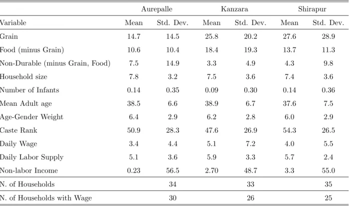
We test homogeneity in risk preferences and efficiency using the Village Level Studies (VLS) started by the International Crops Research Institute for the Semi-Arid Tropics (ICRISAT). This dataset has been chosen for two reasons. First, a good understanding of the effect of idiosyncratic shocks on household welfare is of particular importance in developing countries, where idiosyncratic shocks may have devastating effects on household resources because of the small number of formal markets. Second, several papers in the past have tested efficient risk sharing using this dataset. The results obtained here can therefore be compared with those results.
The ICRISAT started the VLS at six locations in rural India on July 1975. The study added four villages in 1981. In each village 40 households were selected to represent families with different social and economic background. The VLS collected data on production, labor supply, assets, price of goods, monetary, and non-monetary transaction from 1975 to 1985. In addition, the census file contains information on household size, age, education, land holding class (no land, small farm, medium farm and large farm), and caste rankings derived using three different methods. The caste ranking used here is based on Behrman (1988). Townsend (1994) gives a detailed description of the data. We will, therefore, discuss only the issues that are specific to our paper.
The sample used in the estimation is composed of households from only 3 of the 10 villages that were included in the study. These three villages are Aurepalle, Shirapur, and Kanzara. We choose this three villages for two reasons. First, data for these villages are available for the entire sample period. Second, previous studies have focused on these villages.
Monthly household consumption is calculated using the transaction data from the ICRISAT Household Transaction Schedule. The consumption variable is the sum of consumption on grain,
consumption on other food items, namely oil, animal products, fruits and vegetables, and con-sumption on other non-durable goods. The transaction data are collected during each interview. The interview frequency varies. According to the ICRISAT manual, each household should be interviewed at intervals of 3 to 4 weeks. In the data most households are interviewed every month. But there are consecutive interviews that are two weeks apart and consecutive interviews that are two months apart. On average each household has more than 11 interviews each year. The main problem of using the transaction files is that the dates of the interviews differ across households. For example, a household in Aurepalle was interviewed on January 11, February 10, and March 21 in 1980, whereas a different household in the same village was interviewed on January 17, February 13, and March 25 in the same year. This makes it difficult to compare expenditure across different households. To overcome this problem we assume that the rate of consumption is constant between two interviews. Under this assumption we can compute monthly consumption using the consump-tion data from two consecutive interviews. Similarly, the wage and labor supply data are collected at each interview date and then converted into monthly data.
The construction of the wage and labor supply variables for the tests with nonseparable prefer-ences requires a separate discussion. Three different types of employment and wages are recorded by the ICRISAT. The Labor, Draft Animal, and Machinery Utilization Schedule contains informa-tion on hours, days of employment, and wages of individuals entering daily employment outside their own farm. In the Household Transaction Schedule labor income of individuals with regular jobs outside their own farm is recorded, but there is no information on the days and hours of employment. We assume that the data on regular labor income refer to the period covered by the interview and that the individual with the regular job works 8 hours a day for 5 days a week. In the Plot Cultivation Schedule, the ICRISAT collects data on the number of hours supplied by men, women, and children to their own farm and the value of their labor. The value of own labor is imputed by the ICRISAT on the basis of the current village-specific market prices. The information in these three schedules is used to compute monthly household labor supply and wages. Household labor supply is the average number of hours of employment on daily jobs, regular jobs, and jobs on own farm supplied by adult members. Household wages are computed as the average of total labor income earned on any job by adult members divided by the total number of hours. To compute the total time endowmentT and leisure we follow Rosenzweig (1988) and Townsend (1994) and assume that each individual has 26 days per month and 14 hours per day that can be divided between
labor and leisure. The remaining days and hours account for sleep, sickness, and holidays.
The Monthly Price Schedule contains detailed information on monthly prices for each consump-tion item included in the transacconsump-tion files. The price data are used to construct price indices to deflate consumption and wages. To control for household size and age structure, household age-sex weights are constructed following Townsend (1994). The age-sex weights are constructed by adding the following numbers: for adult males, 1.0; for adult females, 0.9; for males aged 13-18, 0.94; for females aged 13-18, 0.83; for children aged 7-12, 0.67; for children aged 4-6, 0.52; for Toddlers 1-3, 0.32; and for infants 0.05. Household consumption is then divided by the weight. The set of demographic variables includes the mean of the ages of household members, their caste, the number of infants, and a constant that captures the unobservable heterogeneity.
The sample covers the period from July 1975 to July 1985 for Aurepalle and from July 1975 to July 1984 for Shirapur and Kanzara. We drop the households that leave the sample before 1985 for Aurepalle and 1984 for Shirapur and Kanzara. This implies that for each household in Aurepalle we have up to 126 observations and for each household in Shirapur and Kanzara up to 114 observation. In all tests, we drop a household if it have fewer than 100 data points.
7.2 Econometric Issues
We estimate the expenditure functions and their differences using the series estimator described in section 5. An important choice is represented by the order of the polynomials. The main variable in the household expenditure function is total expenditureρi,j. It is therefore crucial to allow for
a polynomial in this variable that is flexible enough. We have experimented with polynomials of order between 2 and 5. The outcome of the tests changes substantially when we increase the order from 2 to 3. But the results are stable for polynomials of order greater than 2. The results reported in the paper are for a polynomial of order 3.
The demographic and wage variables are not as important for the outcome of the tests. Since the panel used in the estimation is not long, we have decided to set the order of the polynomial to 1 for all these variables. For the separable case, we have also tested homogeneity in risk preferences and risk sharing with a polynomial of order 2 in the heterogeneity term with similar results. In the nonseparable case an increase in the order of the polynomial to 2 reduces significantly the precision of the estimates since 32 terms plus the terms of the polynomial in the heterogeneity termu must be included.
An increase in the order of the polynomial in u has smaller effects on the precision of the estimates because the interaction betweenuand the other variables is not required in the estimation. We experimented with polynomials of order 1, 2, and 3 with similar findings. The results are reported for a polynomial of order 1.
The set of instruments used to control for endogeneity is composed of lagged rain and lagged total expenditure. The distribution of the test statistics are derived using 500 bootstrap samples. In all the tests the wages and demographic term must be fixed at a particular value. In the tests, these variables are set equal to the household mean. The kernel estimator employed in the efficiency test with excluded variables uses a gaussian kernel. In the efficiency test with increasing expenditure functions, the smoothing parameter is set equal tom.
8
Results With Separable Preferences
In this section, we test homogeneity in risk preferences and efficient risk sharing under the assump-tion that household preferences are separable between consumpassump-tion and leisure. If this restricassump-tion is satisfied, the amount of resources allocated to household i, ρi, corresponds to expenditure on
the consumption good ci and total resources, ρi,j, corresponds to total consumption expenditure
of householdiand j. Homogeneity in risk preferences and efficiency can therefore be tested using only data on consumption.14
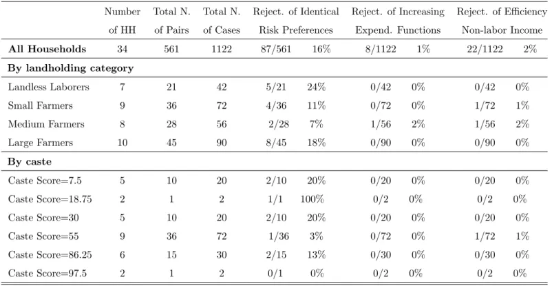
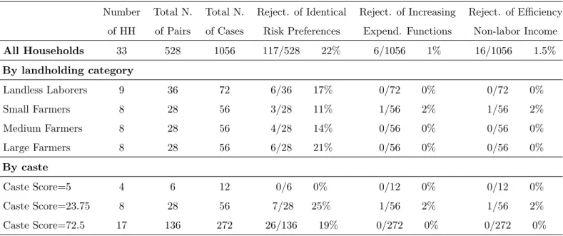
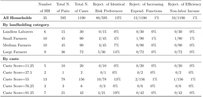
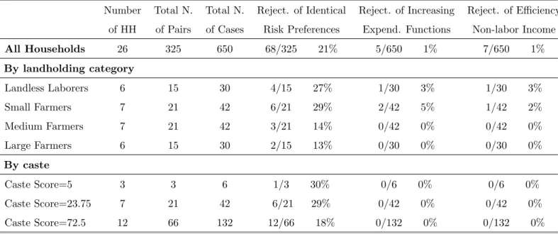
We first test homogeneity in risk preferences. The estimation of the household expenditure functions results indicates that every pair of households can be assigned to one of three different categories: (i) pairs of households whose expenditure functions do not cross; (ii) pairs with ex-penditure functions that cross once; (iii) pairs whose exex-penditure functions cross twice. Figure 6 depicts one pair of households for each category for Aurepalle. The finding that the expenditure functions cross is a first indication that heterogeneity in risk preferences is a significant feature of Indian villages. The outcome of the test of homogeneity in risk preferences discussed in section 6.1 are presented in tables 2-4. Homogeneity in risk preferences is rejected in the three Indian villages. The village with more rejections is Kanzara with 117 cases out of 528, which corresponds to 22% of possible cases. The village with fewer rejections is Shirapur with 80 pairs that reject homogeneity in risk preferences out of 595 possible pairs, which corresponds to 13% of cases. Figure 7 depicts
14The tests can also be implemented using only data on leisure. However, as discussed in Townsend (1994) the ICRISAT leisure and wage data are noisier than the consumption data.
the difference in household expenditures for one of those pairs. It is therefore not surprising that previous papers that have used ICRISAT have rejected efficient risk sharing.
We now focus on the efficiency tests. We first test whether non-labor income affects household expenditure after controlling for pooled resources. We then evaluate whether household expenditure increases with pooled resources.
The outcome of the test of efficiency with excluded variables is presented in columns eight and nine of Tables 2-4. In the three villages efficiency is rejected for a negligible number of households. The village with the largest percentage of rejections is Aurepalle at 2%, with 22 households out of 1122. The village with the lowest percentage of rejections is Shirapur with 1%.
We now proceed to test efficiency using the monotonicity of the expenditure functions. The results of the test are presented in columns six and seven of Table 2-4. The second test of efficiency displays a pattern of rejections that is similar to the excluded variable test. In all villages we reject efficiency for about 1% of households.
These results suggest that if risk preferences are allowed to vary across households, there is very little evidence against efficient risk sharing using the standard testable implication.
9
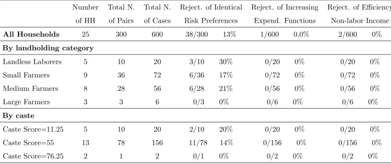
Results With Non-separable Preferences
In this section the tests are implemented by allowing for non-separability between consumption and leisure. In this case, household expenditure differs from the expenditure obtained with separable preferences in two respects. First, the second stage of the Pareto problem implies that household expenditure is also a function of wages, i.e.
ρk=gk¡ρi,j, wi, wj, di,j¢+mk, k=i, j. (11)
This implies that efficiency and heterogeneity in risk preferences can be tested only after the vari-ation produced bydi,j, andwhas been removed. To this end we first estimate semi-parametrically the expenditure functions and their differences. We then fix wages and the heterogeneity term at the household mean and use the changes in ρi,j to perform the tests. A second difference is that
household expenditure ρk is equal to expenditure on consumption ck plus expenditure on leisure
wklk.
We first describe the outcome of the risk preferences test. After controlling for variations in wages, we still find households with expenditure functions that cross one and two times. Figure 10
describes three pairs of households with different crossing patterns. The outcome of the formal test of homogeneity in risk preferences is described in tables 5-7. In the non-separable case 16% of the pairs in Aurepalle, 21% of the pairs in Kanzara, and 13% of the pairs in Shirapur are characterized by expenditure functions that cross.
The results of the efficiency test with excluded variables are reported in the last two columns of table 5-7. In this case, the largest fraction of rejections is in Aurepalle and Kanzara with 1%. Columns six and seven of table 5-7 reports the outcome of the efficiency test with monotone functions. The findings are similar to the excluded variable test.
To summarize, non-separability between consumption and leisure does not change the outcome of the tests. We still find strong evidence against homogeneous risk preferences and little evidence against efficient risk sharing in Indian villages once we allow for different risk preferences across households.
10
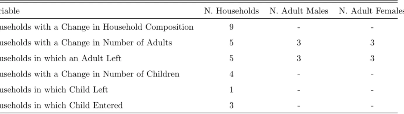
Household Composition and Heterogeneity in Risk Preferences
In this paper we follow the risk sharing literature and we do not allow households to change their composition in response to idiosyncratic and aggregate shocks. The changes in household composition are assumed to be exogenous and they are captures by changes in the age-gender weight discussed in the data section and by changes in observable heterogeneity. If the changes in household composition are in response to shocks, the test of homogeneous risk preferences may capture a different evolution of household composition across households that is not captured by the age-gender weight or observable heterogeneity instead of heterogeneity in risk preferences.In this section we attempt to determine the effect of changes in household composition on the risk preferences test. To that end we test homogeneity in risk preferences by excluding from the sample households that experience a change in the number of members that is not a birth or a death. Table 8 describes the households that are characterized by this type of change. In the data, 9 out of 34 households are characterized by at least one change during the sample period. In 5 of these households one or two adult members left the family during the sample period. In 3 households, one child entered the family and in one household a child left the family during the years 1975-1985.15 The outcome of the risk preferences test for the separable and non-separable
15If we include changes in household composition due to death, the number of households with variation in the number of members increases to 12. Almost all household have at least one birth.