Lumpy investment and variable capacity utilization: firm-level and macroeconomic implications

Faculty of Business, Economics and Social Sciences

Department of Economics

Lumpy investment and variable capacity

utilization: firm-level and macroeconomic

implications

Andreas Bachmann

15-10

September 2015

DISCUSSION PAPERS

Lumpy investment and variable capacity utilization:

firm-level and macroeconomic implications

Andreas Bachmann ∗

University of Bern

September 15, 2015

Abstract

The macroeconomic implications of firms’ lumpy investment behavior are subject to ongoing research. Lumpy investment results from fixed capital adjustment costs which give firms an incentive to reduce the frequency of capital adjustments. However, pre-vious studies have underestimated the lumpiness. Their assumption of constant capital utilization reduces firms’ incentives to undertake large investments as it prevents reserve capacity building. This paper shows that if capacity utilization is allowed to vary, firms optimally undertake larger investments and leave parts of the new capital stock idle for some periods, thereby reducing the frequency of investment activities. Using a dynamic stochastic general equilibrium model with fixed capital adjustment costs, heterogeneous firms, variable utilization, and aggregate technology shocks, I numerically compute firms’ optimal decisions on investment, utilization and labor demand. Compared to the con-stant utilization model, the findings reveal magnified investment lumpiness: Firms adjust capital less frequently, but invest more when they adjust. However, this appears to be of minor macroeconomic relevance: Moments and impulse responses of macroeconomic quantities change in a similar way when variable utilization is introduced in a lumpy or in a frictionless model. New empirical evidence based on firm-level panel data confirms some of the theoretical findings.

JEL Classification: E22, E32, D92

Keywords: lumpy investment, adjustment costs, reserve capacity, utilization, business cycles

∗_{University of Bern, Department of Economics, Schanzeneckstrasse 1, CH-3001 Bern, Switzerland, phone:} +41 31 631 4777, email: [email protected].

1

Introduction

Analyzing the impact of aggregate shocks on aggregate endogenous variables is a major objec-tive of many macroeconomic models. Because aggregate outcomes result from the interaction of individual agents’ choices, macroeconomic dynamics may essentially depend on microeco-nomic frictions and the heterogeneity of ecomicroeco-nomic agents. This has become an important issue in the analysis of investment dynamics because firm-level capital adjustments are char-acterized by substantial frictions and heterogeneity. There are periods of inaction which are occasionally interrupted by large alterations. Such lumpy, i.e., infrequent and large, adjust-ments have been established as a prevalent feature of investment at the establishment level (e.g.,Doms and Dunne,1998,Cooper et al.,1999,Cooper and Haltiwanger,2006, andGourio and Kashyap,2007). This lumpy investment behavior has been widely interpreted as evidence for non-convexities in capital adjustment costs. For example, if capital adjustment is subject to fixed costs, firms are only willing to invest if their capital stock deviates sufficiently from the desired level. Supporting evidence is provided, for example, by Caballero et al. (1995),

Caballero and Engel (1999) and Cooper et al.(1999).

These non-convex adjustment costs and the resulting lumpy investment behavior at the micro level do not necessarily affect macroeconomic dynamics and the impulse responses of aggregate variables. On the one hand, aggregation smooths lumpy investment activities to the extent that they are not synchronized. On the other hand, general equilibrium price move-ments may additionally smooth investment spikes that survive aggregation. Disregarding this second argument, partial equilibrium models suggest that lumpy microeconomic investment is potentially important for aggregate investment (examples include Caballero et al., 1995,

Caballero and Engel,1999,Cooper et al.,1999, andCooper and Haltiwanger,2006). In con-trast, several general equilibrium models find negligible aggregate effects of lumpy investment (e.g., Thomas, 2002, and Khan and Thomas, 2003, 2008). However, this irrelevance result does not generically follow from general equilibrium. To what extent the effect of fixed costs disappear in general equilibrium is a quantitative question that depends on the details of the model calibration (Gourio and Kashyap, 2007). For example, Bachmann et al. (2013) show that lumpy investment can explain a stylized fact of US macroeconomic data, namely the conditional heteroscedasticity of the aggregate investment to capital ratio. This ratio is sub-stantially more responsive to shocks in booms than in recessions. The results of Gourio and Kashyap (2007) are also indicative of lumpiness affecting the impulse responses of aggregate

investment. Bachmann and Ma (2012) andBachmann and Bayer (2014) provide additional examples in which microeconomic lumpiness matters for macroeconomic analysis.

The existing lumpy investment models posit that firms always fully utilize their capital. However, this assumption is delicate in the presence of fixed capital adjustment costs. Firm-level investment and capacity utilization decisions are inherently interrelated. The assumption of constant utilization reduces the firms’ incentives for large investments, resulting in an underestimation of investment lumpiness. In particular, the incentives to build up reserve capacity are attenuated. The following example illustrates this issue. In an environment with long-run technological progress, the firms’ desired capital services increase over time. Absent fixed investment costs, firms can simply adjust their capital stock to the optimal level in each period regardless of whether utilization is variable. In the presence of fixed costs, however, firms have an incentive to reduce the number of capital adjustments. In particular, it may be optimal to invest up to ˜k > k∗, wherek∗ denotes next period’s optimal capital stock absent fixed costs, and to omit investment and the associated fixed costs in the subsequent period. This is the core idea behind lumpy investment: Because of fixed capital adjustment costs, firms have an incentive to invest more than currently needed in order to relieve themselves of the need to readjust too soon. As a consequence, firms prefer rare and large over frequent and small adjustments. However, this key incentive for large investments is attenuated in the existing lumpy investment models by requiring firms to fully utilize their capital. Intuitively, if firms must use their capital stock ˜kin next period’s production, they have an incentive to select ˜k close tok∗. If, in contrast, this assumption of full utilization is dropped, then firms can easily invest up to a capital stock that is considerably larger than k∗. At the same time, they can achieve optimal capital services k∗ by not fully utilizing their large capital stock. To sum up, if forward-looking firms carry out an investment project, they choose the size of the investment big enough such that, once the project is completed, there is some excess or reserve capacity for future growth and no immediate need to undertake the next investment project.

This paper relaxes the delicate assumption of constant capacity utilization, thereby al-lowing for amplified microeconomic investment lumpiness due to reserve capacity building. It contributes to the lumpy investment literature by providing an analysis of (i) how variability in capacity utilization alters firms’ investment decisions and (ii) how, if at all, macroeconomic variables are affected by the enhanced microeconomic lumpiness. For this analysis, I use a

real business cycle (RBC) model with heterogeneous firms, fixed capital adjustment costs and variable utilization. The economy is subject to aggregate productivity shocks. Apart from variability of utilization, the model is closely related to the setup considered by Khan and Thomas (2003). Firms differ in their capital stock and in the current draw of fixed in-vestment costs. They jointly decide on labor demand, utilization, whether to invest at all, and next period’s capital stock (if they invest). The utilization choice is conceptually very different for investing and non-investing firms: It is an intratemporal choice for the former and an intertemporal decision for the latter. The household side, in contrast, is kept simple: Households decide on consumption, labor supply and the amount of shares to buy.

The extension of the lumpy investment model by variable utilization is motivated by at least three additional reasons besides the aforementioned proper consideration of investments in reserve capacity. First, this paper presents new firm-level evidence highlighting the impor-tance of variable utilization for firms’ investment decisions. Using panel data, I show that firm-level capacity utilization has a direct impact on individual firms’ probability of invest-ment. Moreover, there are significant interaction effects with GDP growth. For example, lagged GDP growth only has a positive impact on the investment probability if the utilization rate is sufficiently high. An aggregation exercise demonstrates that forcing firm-level utiliza-tion rates to be constant alters aggregate investment properties across the business cycle. Second, because preferences for smooth consumption restrict the macroeconomic relevance of lumpy investment in general equilibrium, a potentially greater impact of lumpiness might only emerge in models that attenuate the tight link between consumption and investment dynamics. Variable capacity utilization may provide a way to relax this tight link because, in a standard RBC model, it leads to smoother consumption and more volatile investment.1 Third, variable capacity utilization concedes a limited intertemporal choice to firms refraining from paying the fixed adjustment costs. In contrast, many previous studies have assumed that these firms cannot influence the evolution of their capital stock, an assumption that has been criticized.2 In this paper, non-investing firms affect their depreciation rate and, consequently, 1_{An alternative strategy is used byBachmann and Ma(2012), who consider a model with capital goods} heterogeneity to relax the tight link between consumption and investment dynamics and to enhance households’ ability to smooth consumption. Indeed, they find that fixed capital adjustment costs are of macroeconomic relevance. Their results indicate that the response of fixed capital investment to aggregate productivity shocks differs in both magnitude and persistence depending on the presence of fixed capital adjustment costs.

2

For example,Khan and Thomas(2008, p.396) point out that: “. . . as is the convention throughout the literature, there was a stark assumption that nonconvex adjustment costs applied to all capital adjustments irrespective of their size”. Khan and Thomas(2008) address this issue by allowing for low levels of capital adjustment without incurring fixed costs. They assume that the range of investment rates exempt from such

their future capital stock by changing current utilization. In contrast to Khan and Thomas

(2008), their influence on next period’s capital is naturally asymmetric: Non-investing firms cannot increase capital, but reduce its depreciation by lowering utilization.

The results of this paper shed light on individual firms’ investment, utilization and labor decisions in an environment with fixed capital adjustment costs. The findings reveal that variable utilization magnifies lumpiness: Fewer firms invest on average, but the adjusting firms choose a considerably higher capital stock. Moreover, firms with a lot of capital (i.e., firms that have recently invested) choose a utilization rate substantially below the maximum feasible rate. Thus, this paper provides evidence for reserve capacity building which causes enhanced investment lumpiness: Investing firms optimally choose a capital stock that is too large in the short run and partially lies idle. Additional evidence for amplified lumpiness is provided by an analysis of the investment rate distribution, which reveals that if utilization is variable, firm-level investments relative to their capital stock are larger on average, more volatile, more asymmetric and, in particular, feature substantially higher kurtosis.

The variability of utilization also affects firms’ optimal decisions on labor demand and utilization. Additionally, it induces some cyclical differences: First, the target capital level of investing firms increases more strongly with productivity when utilization is variable. Second, the probability of investment fluctuates to a greater extent across the cycle. The latter finding is confirmed by empirical evidence presented in this paper.

Regarding differences in the behavior of investing and non-investing firms, the results indicate that non-investing firms usually choose a substantially lower utilization rate to save capital for future years. Also, their labor demand is slightly lower in many cases.

While this paper’s results establish amplified investment lumpiness at the firm level owing to variable utilization, the macroeconomic consequences of the lumpiness are less clear-cut. Simulation results suggest that, despite the larger investment of those firms that adjust their capital, the means of most macroeconomic variables differ only slightly across the constant and variable utilization model. Regarding the volatility of macroeconomic aggregates, variable utilization has a more pronounced impact. The variables characterizing investment lumpiness (i.e., the target capital of adjusting firms and the fraction of such firms) are more volatile in this paper’s model. The same holds for output, investment, labor, capital, and the investment ratio, whereas consumption becomes less volatile. However, this pattern does not specifically

pertain to the lumpy investment models. Note that allowing for variable capacity utilization also has macroeconomic effects in a model without fixed capital adjustment costs (henceforth labeledfrictionless model). Hence, the important question is whether the enhanced lumpiness caused by variable utilization has an impact beyond the one that can be expected from introducing variable utilization in a frictionless model. The results do not provide evidence in favor of that. The standard deviation of macroeconomic aggregates appears to change in a similar way when variable utilization is introduced in a frictionless or in a lumpy investment model.

A similar conclusion holds for the impulse responses to aggregate technology shocks: The responses of this paper’s model differ considerably from those of the lumpy investment model with constant utilization,3 but are comparable to those of a frictionless model with variable utilization. In particular, the initial responses of output, investment, consumption and em-ployment hardly depend on the existence of fixed capital adjustment costs. However, notable differences pertain to the impulse response functions of capital, utilization and the target cap-ital of investing firms. In this paper’s model, the response of aggregate capcap-ital is larger and more persistent while aggregate utilization initially increases to a smaller extent compared to the frictionless model with variable utilization. The initial response of investing firms’ target capital is even massively larger. Since the response of aggregate investment is similar though, this means that the additional investment in the aftermath of a positive productivity shock is undertaken by few firms which invest a lot rather than all firms that invest a small amount.

The remainder of the paper is structured as follows. Section 2 presents new empirical evidence based on firm-level panel data highlighting the importance of capacity utilization for investment both at the micro and macro level. In section 3, I describe the building blocks of the theoretical model, the competitive equilibrium, the specification and the calibration of the model. The method for the numerical model solution is explained in section 4. The results are discussed in section 5. It presents optimal firm-level decisions on investment, utilization and labor in an environment with variable utilization and fixed capital adjustment costs, and the macroeconomic consequences thereof. Finally, section 6summarizes and concludes.

3_{Inter alia, the amplified lumpiness is apparent in the considerably larger responses of the fraction of} adjusting firms and the target capital of these firms.

2

Empirical Analysis

This section investigates the relevance of variable capacity utilization for both firm-level and aggregate investment. The analysis is based on quarterly firm-level panel data from the KOF Swiss Economic Institute. I use answers to the KOF business tendency survey of the manufacturing industry, a poll of Swiss industrial companies from a wide range of industrial sectors that participate voluntarily.4

The main outcome of interest are two binary indicators about investment. In the sur-vey, firms are asked whether their technical production capacity was (i) increased, (ii) left unchanged, or (iii) decreased in the preceding three months. I use this categorical variable to construct two binary indicators: first, an investment dummy equal to one if production capac-ity was increased and zero if it was left unchanged or decreased and, second, a disinvestment dummy equal to one if production capacity was decreased and zero if it was left unchanged or increased.

The key explanatory variables are lagged firm-level capacity utilization and lagged real GDP growth. Firms are asked to state their average utilization rate of production capacity in the preceding three months. The variable is categorical, ranging from 50% utilization up to 110% in steps of 5 percentage points. Given this rather fine grid of possible answers, I treat the variable as continuous. Real GDP growth rates are obtained from the State Secretariat of Economic Affairs SECO.5

Table 1 shows basic descriptive statistics for my sample. It includes 1824 firms from 2004 Q1 to 2014 Q3 (43 quarters). Not all firms are observed over the entire period. Overall, there are 36328 firm-quarter observations for the investment indicators and 32369 for capacity utilization.

Table 1: Descriptive statistics

Mean SD obs

Investment (yes/no) 13.8% 36328

Disinvestment (yes/no) 4.2% 36328

Capacity utilization 82.3% 14.2 32369

Real GDP growth rate 0.5% 0.6 43

Notes: Mean, standard deviation (SD) and number of observations (obs)

4

For additional information such as sample questionnaires, see http://www.kof.ethz.ch/en/surveys/ business-tendency-surveys/manufactoring/.

5

To investigate how capacity utilization affects investment, I specify a linear panel data model for the investment decision of firmiin periodtwith firm-specific effects and interaction terms as dit= 4 X j=1 βjGDPt−j+ 4 X j=1 γjuit−j+ 4 X j=1 δjGDPt−juit−j +ci+εit, (1)

where dit is the decision on either investment or disinvestment in period t, uit−j denotes

capacity utilization, ci is a firm-specific unobserved effect that may be correlated with the

regressors uit−j, and εit is a time-varying error. Moreover, time dummies are included, but

not shown for readability.6

Different strategies can be used to remove the unobserved effect ci from equation (1). I

use the within transformation, which subtracts the average over time of (1) from the model equation: dit−di·= 4 X j=1 βj(GDPt−j −GDP·) + 4 X j=1 γj(uit−j−ui·) + 4 X j=1 δj(GDPt−juit−j −GDP·ui·) +εit−εi·, (2)

where a dot in the subscript indicates time-averages, e.g., di· = T−1PT_t=1dit. The pooled

OLS estimator of the demeaned equation (2) is called the fixed effects (FE) estimator. Under the assumption of strict exogeneity,

E(εit|GDP1, . . . , GDPT, ui1, . . . , uiT, ci,time dummies) = 0, t= 1, . . . , T, (3)

the FE estimator is consistent and unbiased. Given thatGDP is an aggregate variable whereas

εit is firm-specific, strict exogeneity is likely to hold. However, the firm-specific errorεit may

possibly affect future capacity utilization, rendering u in (2) potentially endogenous.

To solve the potential endogeneity problem associated with FE estimation of (1), I rely

6_{Because the dependent variables are binary, (1) represents a linear probability model. Logit or probit} models are often used to analyze binary choices, but since these models do not easily generalize to the combi-nation of fixed effects and dynamics (as considered in model (4)), I confine the analysis to linear probability models. This type of model has well-known limitations. It implies heteroscedastic errors, which I address by computing heteroscedasticity-robust standard errors. Moreover, estimated probabilities from this model are not restricted to the unit interval. However, because I am interested in estimating mean effects, this issue should not substantially affect the results.

on lagged instruments from the panel. In particular, the first-differenced errorεit−εit−1may

be correlated withuit−1−uit−2, but should be unrelated touit−2 and further lags, which can

therefore be used as instruments. This procedure relies on εit being serially uncorrelated. To

ensure this, I include lagged dependent variables in equation (1) and specify the following linear dynamic panel data model:

dit= p X j=1 αjdit−j + 4 X j=1 βjGDPt−j+ 4 X j=1 γjuit−j+ 4 X j=1 δjGDPt−juit−j+ci+εit, (4)

which additionally includes time dummies. The number of dependent variable lagspis chosen such that εit is serially uncorrelated. p = 1 is sufficient in the model with the investment

dummy as dependent variable whereas p = 2 is needed in the model for the disinvestment dummy.

I estimate (4) using the system GMM estimator proposed by Blundell and Bond (1998), who build on the work ofArellano and Bover(1995). As outlined inArellano and Bond(1991), estimation of (4) may proceed by first-differencing the equation to remove the fixed effect and using dit−2,uit−2 and further lags to instrument ∆dit−1 and ∆uit−1 on the right-hand side.

System GMM augments this so-called difference GMM by additionally using lagged differences as instruments for the level equation.7 Thus, system GMM estimates simultaneously in levels and differences with different instruments for the two equations. The moment conditions are given as follows:

E[dit−l∆εit] = 0, E[uit−l∆εit] = 0, for t≥3, l≥2, (5)

E[∆dit−1(ci+εit)] = 0, E[∆uit−k(ci+εit)] = 0, for t≥3, k= 1, . . . ,4. (6)

I perform the estimation using the Stata command xtabond2 of Roodman(2009b).

The number of instruments is quadratic in the time dimension of the panel because the number of applicable lags in (5) increases withT. As discussed inRoodman(2009a), too many instruments (instrument proliferation) is a common problem in connection with system GMM. It is problematic because many instruments can cause overfitting of endogenous variables and imprecise estimation of the optimal weighting matrix. Because my sample consists of 43 quarters of observations, the empirical analysis based on the system GMM estimator is prone

7

to the problems associated with instrument proliferation. Therefore, I restrict the number of instruments.

I apply two different ways to reduce the number of instruments. The first consists in reducing the moment conditions (5) by considering only a few instead of all available lags. I estimate various model specifications, the largest model using up to the sixth lag as instru-ments. The second way consists in collapsing the instrument set (see Roodman,2009a). The moment conditions (5) and (6) are replaced by

E[dit−l∆εit] = 0, E[uit−l∆εit] = 0, forl≥2, (7)

E[∆dit−1(ci+εit)] = 0, E[∆uit−k(ci+εit)] = 0, fork= 1, . . . ,4, (8)

in which case the instrument count is linear in the time dimension of the panel. Just as (5) and (6), the moment conditions (7) and (8) embody the belief of orthogonality between differenced errors and lagged levels ofdandu, and between errors in levels and lagged differences ofdand

u. However, in contrast to the moment conditions (5) and (6), the estimator only minimizes P

dit−l∆εit and Puit−l∆εit for each l rather than for each l and t separately. Similarly,

P

∆dit−1(ci+εit)andP∆uit−k(ci+εit)are only minimized in total, not separately for each

t. Thus, less information is conveyed by a collapsed instrument set. On the other hand, no lags are actually dropped, which is a potential advantage over the approach of reducing the number of instruments by capping the number of lags used as instruments.

Applying the system GMM estimator involves many specification choices. Therefore, it is important to check the robustness of the results. I use various specifications: Anderson and Hsiao(1982) difference and level estimators, which use only either the most recent lagged difference or lagged level as instruments for the first difference of equation (4), the difference GMM estimator proposed by Arellano and Bond (1991), and the system GMM estimator discussed above with either a restricted number of lags used as instruments or with a collapsed instrument set. Despite some quantitative differences, the results are qualitatively robust to different specifications of the GMM estimator. The aggregate findings (presented in figures1

and 2 below) and the resulting conclusions are even more robust. First stage regressions of level variables on first-differences and of first-differenced variables on lagged levels clearly confirm the strength of the instruments used in the different model specifications.

investment indicator as dependent variable. Table 3 shows the corresponding results for the disinvestment dummy. Columns (1) and (3) contain the estimates for the models without interaction terms. The estimated coefficients are of the expected sign: Both recent GDP growth and utilization have a positive impact on the probability of investment and a negative impact on the probability of disinvestment.

Columns (2) and (4) of tables2and3present the estimates for the models including inter-action terms. The findings show a significant impact of capacity utilization on the probability of investment. Moreover, some of the interaction terms are significant as well, indicating that the impact of lagged GDP growth on the probability of investment or disinvestment hinges on the firm-level utilization rate. For example, according to the results in column (2) of ta-ble 2, the effect of an increase in GDP growth by one percentage point on the probability of investment two quarters later is given by:

∂dit

∂GDPt−2

=−0.0548 + 0.0009uit−2. (9)

Thus, the impact of GDPt−2 on the investment probability is zero at a utilization rate of

60%. For firms with a utilization rate of 100%, however, an increase in GDP growth by one percentage point increases the probability of investment two quarters later by 3.6 percentage points. Thus, lagged GDP growth only has a positive effect on the investment probability if the utilization rate is sufficiently high.

Overall, the findings in tables 2 and 3 show that firm-level investment decisions across the business cycle crucially depend on capacity utilization. Not only does the investment decision directly depend on utilization, but the rate of capacity utilization also influences how firm-level investment responds to aggregate GDP growth.

In the remainder of this section, I assess whether the relevance of variable capacity uti-lization for investment decisions at the firm-level carries over to aggregate quantities. To this end, I compare different aggregate investment and disinvestment time series, which are constructed as follows: The regression results from column (4) in table 2 are used to predict the probability of investment, which is then aggregated across firms using employment-based weights. Moreover, an alternative probability of investment is predicted with capacity uti-lization restricted to be fixed at the firm-specific mean. This alternative probability is also aggregated across firms. The resulting employment-weighted fractions of investing firms are

Table 2: Regression results for investment dummy FE GMM (1) (2) (3) (4) GDPt−1 0.0214*** -0.0375 0.0187*** -0.0328 (0.0073) (0.0259) (0.0072) (0.0483) GDPt−2 0.0215*** -0.0548** 0.0207** -0.0498 (0.0076) (0.0228) (0.0080) (0.0313) GDPt−3 0.0116 0.0162 0.0020 0.0149 (0.0078) (0.0249) (0.0086) (0.0345) GDPt−4 0.0075 -0.0405 0.0195*** -0.0576 (0.0163) (0.0282) (0.0075) (0.0414) uit−1 0.0026*** 0.0023*** 0.0022*** 0.0019*** (0.0003) (0.0004) (0.0004) (0.0005) uit−2 0.0006* 0.0001 0.0004 0.0000 (0.0003) (0.0003) (0.0004) (0.0004) uit−3 0.0007** 0.0008** 0.0009** 0.0010** (0.0003) (0.0004) (0.0004) (0.0004) uit−4 0.0001 -0.0002 0.0002 -0.0003 (0.0003) (0.0003) (0.0004) (0.0005) GDPt−1uit−1 0.0007** 0.0006 (0.0003) (0.0006) GDPt−2uit−2 0.0009*** 0.0008** (0.0003) (0.0004) GDPt−3uit−3 0.0000 -0.0001 (0.0003) (0.0004) GDPt−4uit−4 0.0006** 0.0009* (0.0003) (0.0005) dit−1 0.2021*** 0.2005*** (0.0162) (0.0161) Number of observations 18063 18063 17055 17055 Number of firms 1151 1151 1124 1124

Arellano-Bond test for AR(2): p-value 0.354 0.378

Arellano-Bond test for AR(3): p-value 0.935 0.941

Hansen test: p-value 0.783 0.772

Source: KOF Business Tendency Survey Manufacturing Industry 2004-2014, own calculations.

Notes: All models include year dummies. Cluster-robust standard errors in parantheses. (3) and (4) are estimated by theBlundell and Bond(1998) system GMM estimator with lagged dependent variable and lagged utilization (and interactions) instrumented. The instrument set is collapsed (cf. Roodman,2009a), which results in an instrument count of 228 and 371 for (3) and (4). The third and second last line show thep-values for theArellano and Bond(1991) autocorrelation tests of order 2 and 3. The last line presents thep-value of the over-identification test proposed byHansen(1982).

*p <0.1. **p <0.05

Table 3: Regression results for disinvestment dummy FE GMM (1) (2) (3) (4) GDPt−1 -0.0099** -0.0138 -0.0093** 0.0368 (0.0038) (0.0198) (0.0039) (0.0303) GDPt−2 -0.0224*** -0.0248 -0.0212*** -0.0088 (0.0070) (0.0230) (0.0072) (0.0277) GDPt−3 0.0010 0.0276 0.0139* 0.0626** (0.0064) (0.0204) (0.0078) (0.0247) GDPt−4 -0.0011 -0.0532** -0.0045 -0.0003 (0.0100) (0.0212) (0.0069) (0.0280) uit−1 -0.0013*** -0.0014*** -0.0011*** -0.0008** (0.0003) (0.0003) (0.0003) (0.0003) uit−2 -0.0003 -0.0003 -0.0004 -0.0003 (0.0002) (0.0003) (0.0003) (0.0003) uit−3 0.0003* 0.0005** 0.0000 0.0003 (0.0002) (0.0003) (0.0002) (0.0003) uit−4 0.0004* 0.0001 0.0000 0.0001 (0.0002) (0.0003) (0.0003) (0.0003) GDPt−1uit−1 0.0000 -0.0005 (0.0002) (0.0003) GDPt−2uit−2 0.0000 -0.0002 (0.0003) (0.0003) GDPt−3uit−3 -0.0003 -0.0006** (0.0002) (0.0003) GDPt−4uit−4 0.0006*** 0.0000 (0.0002) (0.0003) dit−1 0.2637*** 0.2625*** (0.0236) (0.0236) dit−2 0.0658*** 0.0643*** (0.0202) (0.0202) Number of observations 18063 18063 16973 16973 Number of firms 1151 1151 1124 1124

Arellano-Bond test for AR(2): p-value 0.346 0.314

Arellano-Bond test for AR(3): p-value 0.437 0.412

Hansen test: p-value 0.550 0.860

Source: KOF Business Tendency Survey Manufacturing Industry 2004-2014, own calculations.

Notes: All models include year dummies. Cluster-robust standard errors in parantheses. (3) and (4) are estimated by theBlundell and Bond(1998) system GMM estimator with lagged dependent variable and lagged utilization (and interactions) instrumented. The instrument set is collapsed (cf. Roodman,2009a), which results in an instrument count of 265 and 408 for (3) and (4). The third and second last line show thep-values for theArellano and Bond(1991) autocorrelation tests of order 2 and 3. The last line presents thep-value of the over-identification test proposed byHansen(1982).

*p <0.1. **p <0.05

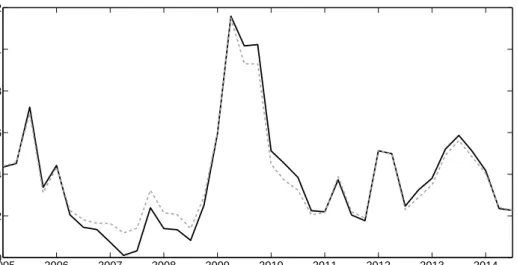
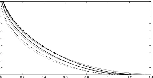
plotted in figure 1.8 The figure reveals that restricting utilization to be constant results in a different fraction of investing firms. The difference is cyclical: The restricted series un-derpredicts investment activity in booms and overpredicts it in periods of low GDP growth. Figure2 shows an analogous analysis for the fraction of firms with negative investment. The prediction of this fraction appears to be too low in recessions and too high in booms if uti-lization is fixed. Figure 3 plots the difference in the predicted fraction of investing firms if utilization is allowed to vary or kept constant. Figure 4 depicts the corresponding difference in the predicted fraction of firms with negative investment. The differences are significant at the one percent level.9

The aggregate results for the fraction of investing firms do hardly depend on the underlying econometric model (FE or system GMM): The difference between the predicted fraction of investing firms when utilization is either variable or forced to be constant is almost identical for both models (cf. figures 3 and 17). Clearly, this difference is cyclical. This also holds for the predicted fraction of firms with negative investment, although the difference between the FE and the system GMM results is more pronounced (cf. figures 4and 18). The results depicted in figures 1 to 4 are robust to the use of alternative instrument sets in the system GMM estimation. 20050 2006 2007 2008 2009 2010 2011 2012 2013 2014 0.05 0.1 0.15 0.2 0.25 0.3

Fraction of investing firms

Figure 1: The fraction of investing firms when capacity utilization is fixed (gray dashed line) or variable (black solid line). The estimation is based on column (4) in table2.

8

AppendixAcontains figures analogous to1to4, but based on the FE (column (2) in the tables2and3) instead of the system GMM results.

9_{This holds for the differences plotted in figures3,4,17and18. Confidence intervals are computed using} the delta method. They are very narrow and therefore not depicted.

20050 2006 2007 2008 2009 2010 2011 2012 2013 2014 0.02 0.04 0.06 0.08 0.1 0.12

Fraction of firms with negative investment

Figure 2: The fraction of firms with negative investment when capacity utilization is fixed (gray dashed line) or variable (black solid line). The estimation is based on column (4) in table3.

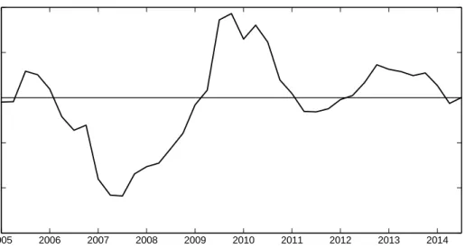
2005 2006 2007 2008 2009 2010 2011 2012 2013 2014 −2.5 −2 −1.5 −1 −0.5 0 0.5 1 1.5 2 2.5 Percentage points

Figure 3: Difference in the predicted fraction of investing firms when utilization is variable or fixed. The difference is based on the GMM model (column (4) in table2).

2005 2006 2007 2008 2009 2010 2011 2012 2013 2014 −1.5 −1 −0.5 0 0.5 1 Percentage points

Figure 4: Difference in the predicted fraction of firms with negative investment when utilization is variable or fixed. The difference is based on the GMM model (column (4) in table3).

Overall, the empirical analysis suggests that capacity utilization is a relevant variable in lumpy investment models. Compared to a fixed capacity utilization, high utilization rates in booms cause a larger fraction of firms to invest and a lower fraction to disinvest, which (depending on the size of the capital adjustment) may have macroeconomic effects. Analo-gously, low utilization rates in recessions cause a smaller fraction of firms to invest and a larger fraction to disinvest. In the light of this empirical evidence, capacity utilization appears to be an important ingredient in models assessing the relevance of lumpy firm-level investment for macroeconomic investment.

3

Theoretical model

I consider an RBC model with variable capacity utilization, heterogeneous firms and capital adjustment costs. Within any period, these capital adjustment costs are fixed at the level of a production unit, but may differ across units. As a consequence, some production units will undertake capital adjustments while others will not, resulting in firm heterogeneity with respect to the capital stock.

The model features long-run growth due to technological progress. Let γ denote the gross growth rate of the economy along the balanced growth path caused by trend growth in productivity. In the following exposition, I consider the detrended model, i.e., all variables measured in units of output are deflated.

Overall, the framework is closely related to the setups considered by Khan and Thomas

(2003,2008), Bachmann et al.(2013) and Bachmann and Bayer(2014). The main departure from these papers is to allow for variable capacity utilization, thereby introducing an intensive margin along which capital input to production can be adjusted. The following sections describe the model in detail.

3.1 Firms

The economy consists of a continuum of production units, henceforth labeled firms.10 Because I do not model firms’ entry and exit decisions, the mass of firms can be normalized to one. At any date, each firm is characterized by its predetermined capital stockkand its fixed cost of investmentκ∈[0, B]. This fixed cost is denominated in hours of labor. Thus, a firm deciding to adjust its capital stock incurs costs of κw, where wdenotes the real wage. In each period,

κ is drawn from a time-invariant distribution G, which is continuous and has support[0, B]. The distribution G is common across firms. The draws from G are independent both over time and across firms.

There is a single commodity in the economy that can be consumed or invested. Each firm produces this commodity using capital services and labor as inputs. Capital services are given by the product of the capital stock k and capacity utilization u. In each period, k is predetermined while u can be adjusted up to an upper boundu¯.11 Labor n can be adjusted without frictions. Each firm’s production is described by the function:

y=zF(ku, n), (10)

which satisfies the following properties:12

F1 >0, F2 >0, F11<0, F22<0, F12≥0.

z denotes exogenous aggregate productivity which is common across all firms. As in Khan

10

Different interpretations of the size of production units are possible. For example,Cooper and Haltiwanger (2006) and Khan and Thomas(2008) assume that the production units in the model correspond to plants, whileBloom(2009) sets the number of productive units per firm at 250 for his simulation.

11_{Specifically, utilization can amount to 100% at most. However, I calibrate the model such that the steady} state utilization rate equals one in the model without capital adjustment costs. Because of this normalization,

¯

u >1andu∈(1,u¯]indicates utilization rates which exceed steady state utilization in the frictionless model. 12_{Functions with subscript numbers represent derivatives of the function with respect to the indicated} arguments.

and Thomas (2003, 2008), I assume that z follows a Markov chain with finite states z ∈

{z1, . . . , zNz},Pr(z

0_=z

j|z=zi) =πji and PN_j=1z πji= 1 for each i= 1, . . . , Nz.13

The aggregate state of the economy is described by(z, µ)whereµdenotes the distribution of capital across firms. This distribution of firm-level capital evolves according to a law of motion Γ which depends on the aggregate state of the economy: µ0 = Γ(z, µ). Γ will be described in more detail below.

Each firm’s capital stock evolves according to:

γk0 = (1−δ(u))k+i. (11)

γ denotes the steady state gross growth rate of capital. Depreciation is an increasing, convex function of utilization, which is a standard way to model the costs associated with higher utilization (cf. King and Rebelo,2000). idenotes investment. i6= 0requires paying the fixed costs of κw.

The firms maximize the expected sum of discounted profits by making a discrete decision about investment and by choosing labor n, utilization u, and next period’s capital stock k0. These decisions are interrelated. The optimal choices of labor and utilization may differ for investing and non-investing firms. This difference is apparent for capacity utilization: For firms that choose to invest, the decision onu is intratemporal and independent of the choice onk0. In contrast, the choice onuis an intertemporal decision for non-investing firms because

udeterminesk0 through equation (11). Thus, unlike inKhan and Thomas(2003),Bachmann et al. (2013) or Bachmann and Bayer(2014), non-investing firms can make an intertemporal decision, albeit the choice set is limited to the attainable values of next period’s capital stock,

k0 ∈[(1−δ(¯u))k/γ,(1−δ(0))k/γ].

Let v1(k, κ;z, µ) represent the expected discounted value of a firm with individual state variableskandκwhen the aggregate state of the economy is(z, µ). The expected value prior to the adjustment cost draw κ amounts to

v0(k;z, µ) =

Z B

0

v1(k, κ;z, µ)G(dκ). (12)

Let dzj(zi, µ) denote the discount factor that firms apply to their future value if aggregate

13_{Throughout this paper’s model description, time subscripts are omitted and next period’s variables are} denoted with a prime.

productivity isziin the current andzj in the next period. With this notation, the optimization

problem of a firm can be stated as dynamic programming problem:

v1(k, κ;z, µ) = max sup u,n [zF(ku, n)−wn+ (1−δ(u))k]−κw + sup k0 −γk0+E[dz0(z, µ)v0(k0;z0, µ0)]; (13) sup u sup n (zF(ku, n)−wn) +E dz0(z, µ)v0 (1−δ(u))k γ ;z 0_{, µ}0 .

The outer maximization represents a binary choice on investing. Let I∗(k, κ;z, µ) ∈ {0,1}

denote the optimal binary choice. The last line in (13) describes the optimization problem of a firm that decides not to adjust its capital stock. Such a firm faces an intratemporal choice on labor n and an intertemporal choice on utilization u, which affects current production

zF(ku, n)and next period’s capitalk0= (1−δ_γ(u))k. The associated policy functions are denoted

by nf_N(k;z, µ) and uN(k;z, µ), respectively.14 Lines two and three in (13) represent the

optimization problem of a firm that decides to adjust its capital stock, thereby incurring fixed costs ofκw. The problem is formulated as if investing firms sell their capital stock remaining after depreciation and purchase γk0. This formulation is equivalent to merely subtracting investment from current profits, but it is more convenient because it reveals that the decisions onk0 on the one hand as well asnanduon the other hand are separable. The optimal choice of uand nis intratemporal and does not depend on the choice on next period’s capital. The associated policy functions are denoted uI(k;z, µ) and nfI(k;z, µ). Similarly, the optimal k0

is independent of the choices on u and n. In fact, (13) reveals that the optimal choice onk0

is also independent of k and κ. Therefore, it does not depend on any firm-specific variable, but only on the aggregate state of the economy. As a result, any firm choosing to undertake capital adjustment will choose the same capital stock, denoted by k∗(z, µ).

There is an equivalent, but simpler representation of the dynamic programming problem in (13) (seeKhan and Thomas,2003,2008). This representation incorporates optimality con-ditions from the households and competitive equilibrium concon-ditions. Therefore, I will proceed by presenting the household sector (section 3.2), characterizing the competitive equilibrium 14_{The superscriptf is used to differentiate labor choices of firms from those of households. The subscript} N indicates non-investing firms. In contrast, subscriptI will indicate investing firms.

(section 3.3) and then analyzing the optimality conditions from the simplified dynamic prob-lem (section 3.4). In section 3.5, I finally present the specification and calibration of the functions and parameters of the model.

3.2 Households

The economy is populated by a continuum of identical households.15 Their wealth is held as (one-period) shares in firms, which are denoted using the measure λ. Thus, the households own the portfolio of firms in the economy. In each period, households choose consumption

C and supply laborN. Moreover, they decide on the amount of new shares λ0(k0) to buy of firms which begin the next period with a capital stock ofk0. Economically, this is a portfolio choice problem with infinitely many assets indexed by k0. The optimization problem is given as follows: W(λ;z, µ) = sup C,N,λ0U(C,1 −N) +βEW(λ0;z0, µ0) (14) s.t. C+ Z K ρ(k0)λ0(dk0)≤wN + Z K v0(k)λ(dk),

with discount factor β <1and where U(C,1−N) satisfies the following properties:

U1 >0, U2 >0, U11<0, U22≤0.

w denotes the real wage,ρ(k0) the price of new shares, and capital is defined onK ⊆R+.

Let p denote the Lagrange multiplier associated with the constraint in the optimization problem (14). The first order conditions for households’ optimal choices are standard and given as follows:

U1(C,1−N) =p, (15)

U2(C,1−N) =pw, (16)

pρ(k0) =βEv0 0(k0)p0, for eachk0 ∈ K. (17)

Let C(λ;z, µ) and Nh(λ;z, µ) denote households’ choice of consumption and labor, respec-tively. Moreover, letΛh(k0, λ;z, µ)denote the amount of shares that households buy of firms

15

which begin the next period with capitalk0.

3.3 Recursive Competitive Equilibrium

A recursive competitive equilibrium is a set of functions

w, d, ρ, v0, v1, k∗, nf_I, nf_N, uI, uN, I∗, W, C, Nh,Λh,Γ

that solve the firms’ problem (13), the households’ problem (14) and clear all markets. In particular, the set of functions satisfies:

(i) Firm optimality: Taking w, d and Γ as given, v0(k;z, µ) and v1(k, κ;z, µ) satisfy (12) and (13) with corresponding policy functions I∗(k, κ;z, µ),n_Nf (k;z, µ),uN(k;z, µ),

nf_I(k;z, µ),uI(k;z, µ) and k∗(z, µ).

(ii) Household optimality: Taking w, ρ, v0 and Γ as given, W(λ;z, µ) satisfies (14) with corresponding policy functions C(λ;z, µ),Nh(λ;z, µ) and Λh(k0, λ;z, µ).

(iii) Asset market clearing: The quantity of “capital k0 shares” bought corresponds to the mass of firms with capital k0, i.e., Λh(k0, µ;z, µ) =µ0(k0) for each k0∈ K.16

(iv) Labor market clearing: Labor supply is equal to labor demand for production and fixed costs of capital adjustment, which is denoted in units of labor:

Nh(µ;z, µ) = Z K Z B 0 nf_N(k;z, µ)(1−I∗(k, κ;z, µ)) +nf_I(k;z, µ)I∗(k, κ;z, µ)G(dκ)µ(dk) + Z K Z B 0 I∗(k, κ;z, µ)κG(dκ)µ(dk). 16

The household sector can be summarized by a representative household. Therefore, the measureλ of shares will coincide with the distribution of firm-level capitalµin equilibrium. Thus, I replaceλbyµin the household’s policy functions.

(v) Goods market clearing: Consumption and gross investment add up to output: C(µ;z, µ) + Z K Z B 0 (γk∗(z, µ)−(1−δ(uI(k;z, µ)))k)I∗(k, κ;z, µ)G(dκ)µ(dk) = Z K Z B 0 zF kuN(k;z, µ), nfN(k;z, µ) (1−I∗(k, κ;z, µ)) +zFkuI(k;z, µ), nfI(k;z, µ) I∗(k, κ;z, µ) ! G(dκ)µ(dk).

(vi) Model consistent dynamics: The evolution of the firm-level capital distribution, µ0 = Γ(z, µ), is induced by the exogenous process forzas well as optimal firm choices affecting next period’s capital, namely k∗(z, µ),I∗(k, κ;z, µ) and uN(k;z, µ):

µ0(k0) = Γ(z, µ) = Z n (k,κ)|k0₌(1−δ(uN(k;z,µ)))k γ andI ∗_{(k,κ;z,µ)=0}o G(dκ)µ(dk) + Z {(k,κ)|k0_=k∗_(z,µ)andI∗_{(k,κ;z,µ)=1}} G(dκ)µ(dk).

The first integral in the above expression integrates over all combinations of k and κ

for which firms optimally choose not to invest and which result in next period’s capital beingk0. The second integral is only relevant fork0 =k∗(z, µ)and zero fork0 6=k∗(z, µ). It integrates over all combinations ofkandκfor which firms optimally choose to invest. This mass of the current capital distribution shifts tok∗(z, µ) in the next period.

3.4 Simplified Dynamic Problem

The firms’ optimization problem can be simplified using equilibrium implications of household utility maximization (see Khan and Thomas,2003,2008). The arising problem is equivalent to the model presented in the previous sections, but consists of a single Bellman equation instead of (13) and (14), which simplifies equilibrium calculation.

The first step of this reformulation consists in finding equilibrium real wages and intertem-poral prices using household optimality and general equilibrium conditions. An expression for the equilibrium real wage is obtained by combining the first order conditions (15) and (16):

w(z, µ) = U2(C,1−N)

U1(C,1−N)

, (18)

market clearing with the household budget constraint leads to the following equation: C+ Z K ρ(k0)µ0(dk0) =wN+ Z K v0(k)µ(dk) =wN + Z K Z B 0 v1(k, κ)G(dκ)µ(dk).

Next, I plug in for v1 and use labor and goods market clearing as well as model consistent dynamics. This results in the relation

Z K ρ(k0)µ0(dk0) = Z KE dz0v0 0(k0)µ0(dk0).

Finally, solving the household first order condition (17) for ρ(k0) and substituting it in the above expression yields:

Z KE βp0 p v 0 0_(k0₎ µ0(dk0) = Z KE dz0v0 0(k0)µ0(dk0).

Thus, the discount factor applied by firms is equal to

dz0(z, µ) = βp

0_(z0_{, µ}0₎

p(z, µ) , (19)

wherep(z, µ) equals marginal utility of consumption.

FollowingKhan and Thomas(2003, 2008), I use the discount factor implied by equation (19) to write the firms’ optimization problem in terms of household utils instead of physical output units:17 V1(k, κ;z, µ) = max sup u,n [zF(ku, n)−wn+ (1−δ(u))k]p−κwp + sup k0 −γk0p+βE[V0(k0;z0, µ0)]; (20) sup u sup n (zF(ku, n)−wn)p+βE V0 (1−δ(u))k γ ;z 0 , µ0 ,

where the price firms use to value their current output is given by p = U1(C,1−N), real

17_{For notational clarity, letV}0 _andV1_{denote the value functions associated with the problem in terms of}

wages are determined by w= U2(C,1−N) U1(C,1−N), and V0(k;z, µ) = Z B 0 V1(k, κ;z, µ)G(dκ). (21)

Optimal labor and capacity utilization choices of an investing firm (nf_I anduI) depend on

the aggregate state (z, µ) and the individual capital stock k. They are characterized by the following first order conditions:

w=zF2(kuI, nfI), (22)

δu(uI) =zF1(kuI, nfI). (23)

The optimal capital choicek∗of investing firms is independent of current capitalkand capital adjustment costsκ and satisfies:

γp=βEV10(k

∗

;z0, µ0). (24)

Thus, all investing firms choose the same capital stock for the next period. The target capital

k∗ depends on the aggregate state(z, µ).

The first order conditions for non-investing firms are given by

w=zF2(kuN, nfN), (25) pzF1(kuN, nf_N) = 1 γδu(uN)βE V₁0 (1−δ(uN))k γ ;z 0 , µ0 . (26)

These conditions determine optimal employment and capacity utilization (nf_N and uN) as a

function of kand (z, µ).

Finally, the binary investment decision is based on the comparison of the expected value of adjusting capital and incurring the fixed costs on the one hand with the expected value of foregoing adjustment on the other hand. The firm invests if

where V_N∗(k;z, µ)≡(zF(kuN, nf_N)−wnf_N)p+βE V0 (1−δ(uN))k γ ;z 0_{, µ}0 , (28) V_I∗(k;z, µ)≡(zF(kuI, nf_I)−wnf_I + (1−δ(uI))k)p−γk∗p+βEV0(k∗;z0, µ0). (29)

It follows that a firm invests if and only if its fixed cost draw κ is below a certain threshold, namely if κ≤κ¯(k;z, µ) = min V_I∗(k;z, µ)−V_N∗(k;z, µ) w(z, µ)p(z, µ) ;B . (30)

This amounts to areservation price orreservation cost strategy, i.e., there is a maximum cost of ¯κ(k;z, µ)w(z, µ)p(z, µ) which a firm with capital k is willing to pay for the possibility to adjust its capital.

Given the investment decision described in (30), the cross-sectional distribution of firm-level capital evolves according to the following law of motion:

µ0(k0) = Γ(z, µ) = Z n k|k0₌(1−δ(uN(k;z,µ)))k γ o(1−G(¯κ(k;z, µ)))µ(dk) + Z K 1{k0 =k∗(z, µ)}G(¯κ(k;z, µ))µ(dk). (31)

1{k0 = k∗(z, µ)} is an indicator function equal to one for k0 = k∗(z, µ) and zero otherwise. Thus, the mass R_KG(¯κ(k;z, µ))µ(dk) of the current capital distribution is shifted to k0 =

k∗(z, µ). For any other value ofk0, only the first line in (31) is relevant.

and labor as follows: C(z, µ) = Z K " zFkuN(k;z, µ), nf_N(k;z, µ) (1−G(¯κ(k;z, µ))) +zFkuI(k;z, µ), nfI(k;z, µ) G(¯κ(k;z, µ)) (32) −(γk∗(z, µ)−(1−δ(uI(k;z, µ)))k)G(¯κ(k;z, µ)) # µ(dk), N(z, µ) = Z K " nf_N(k;z, µ) (1−G(¯κ(k;z, µ))) +nf_I(k;z, µ)G(¯κ(k;z, µ)) + Z ¯κ(k;z,µ) 0 κG(dκ) # µ(dk). (33)

Uniqueness of the goods and labor market equilibrium is likely to hold, but not guaranteed. AppendixCcontains some general considerations on uniqueness in lumpy investment models as well as steady state and simulation results on uniqueness for this paper’s model specification and calibration.

3.5 Specification and Calibration

The specification of preferences and technology closely follows the literature on lumpy invest-ment. The model is calibrated to match annual data from Germany. Unfortunately, I do not have access to a dataset with quantitative firm-level data on both utilization and invest-ment.18 Therefore, I cannot re-calibrate the lumpy investment model for the case of variable utilization. Instead, I choose most parameters according toBachmann and Bayer(2014), who estimate or calculate many parameters directly from German firm-level or national accounts data.

In accordance with the literature on lumpy investment models (includingThomas,2002,

Khan and Thomas, 2003, 2008, Bachmann et al., 2013, and Bachmann and Bayer, 2014), I assume that the firms’ production function takes a Cobb-Douglas form with decreasing returns to scale,

zF(ku, n) =z(ku)θnν, withθ >0, ν >0, θ+ν <1, (34)

18_{The datasets used in previous studies do not include information on utilization while the dataset used in} section2of this paper contains utilization, but only qualitative information on investment.

and that the representative household’s period utility function is additively separable and linear in labor:

U(C,1−N) = log(C) +A(1−N). (35)

This type of utility function results from the standard indivisible labor model in the spirit of Hansen (1985) and Rogerson (1988). In this model, each individual can either work some given positive number of hours or not at all. Hansen (1985) shows that the representative household in such an economy has a utility function as given in (35).

The depreciation function is specified followingRíos-Rull et al.(2012):

δ(ut) =δ0+δ1

u1+1_t /ξ−1. (36)

With δ1 >0 andξ >0, this depreciation function is increasing and convex in ut, a common

way to model the costs of variable capacity utilization (cf. King and Rebelo,2000). Moreover, this specification includes fixed capacity utilization as a special case ifξ →0.

Given the functional forms specified in (34), (35) and (36), some of the optimality condi-tions derived in section3.4 can be simplified as follows:

p= 1 C, (37) w= A p, (38) nf_I = ν 1+ξ(1−θ)_z1+ξ_θξθ_kθ w1+ξ(1−θ)_[δ 1(1 + 1/ξ)]ξθ !_1+ξ(1−θ1_)−ν(1+ξ) , (39) uI= " θzkθ−1_(nf I)ν δ1(1 + 1/ξ) #_1+ξ(1ξ_−θ) , (40) nf_N = νz(kuI)θ w ₁−1ν , (41) uN =       γθpz1−1ν_k θ 1−ν−1_ν ν 1−ν δ1(1 + 1/ξ)βE " V0 1 1−δ0−δ1 u1+1_N /ξ−1k γ ;z0, µ0 !# w1−νν       ξ 1+ξ(1−₁₋θ_ν) . (42)

real wage (38) is determined by the marginal rate of substitution of leisure for consumption. (39) and (40) determine optimal choices of labor and utilization of firms that adjust their capital stock. Labor demand of non-investing firms is characterized by (41). (42) implicitly determines the utilization rate of these firms.

Following the literature (e.g., Thomas,2002, Khan and Thomas, 2003, 2008, Bachmann et al., 2013, and Bachmann and Bayer, 2014), I assume the fixed costs of investment to be drawn from a uniform distribution G(κ) = κ/B. This assumption is not innocuous.19 Nevertheless, I rely on it because this facilitates comparing my findings to those of other studies.

My calibration of the parameters heavily relies onBachmann and Bayer(2014). In partic-ular, the values of the parametersA,B,β,γ,δ0,θandν are identical to their model.20 Since

Bachmann and Bayer (2014) do not consider variable utilization, I rely on other sources for the calibration of u¯ and the depreciation function’s parameters δ1 and ξ. As noted by King

and Rebelo (2000) and Ríos-Rull et al. (2012), little is known about ξ. I use ξ = 1, which approximately corresponds to the point estimate from Basu and Kimball (1997). Following

Ríos-Rull et al. (2012), δ1 is chosen such that the steady state utilization rate equals one in

the model without capital adjustment costs. This normalization simplifies the comparison of this paper’s model with the frictionless model. Given a steady state utilization of one, u¯

is determined using the data from the KOF Swiss Economic Institute analyzed in section 2. Mean firm-level utilization equals 82.3% in the dataset. Maximum feasible utilization is com-puted as u¯ = 100/82.3 = 1.215, 21.5% above the frictionless model’s steady state. Finally, the Markov chain for aggregate productivity is chosen as an approximation to a continuous AR(1) process with Gaussian white noise innovations:

ln(z0) =ρzln(z) +ε0, withε0 ∼ N(0, σ2z),|ρz|<1. (43)

19

Indeed, considering a different distribution,Gourio and Kashyap(2007) find macroeconomic effects result-ing from fixed capital adjustment costs and investment lumpiness at the firm level. Their preferred calibration features a “compressed” distribution, i.e., many firms bunch around two levels of fixed cost. With many firms facing a similarly sized fixed costs, it is possible that an aggregate shock pushes a lot of firms across the threshold from not investing to investing.

20

B, the upper bound of the fixed cost distribution, has been calibrated very differently in the literature. E.g.,Thomas(2002) andKhan and Thomas(2003,2008) choose a substantially lower value forB. Nevertheless, the choice of B = 0.2does not appear to be too large because, in the steady state of this paper’s model, it leads to expenditure on adjustment costs that amount to approximately 4% of investment spending. This is still considerably lower than suggested in Gourio and Kashyap(2007), who report average adjustment costs of roughly 7.5% of investment based on the findings ofCooper and Haltiwanger(2006).

I rely on the discretization procedure inTauchen(1986) with nine grid points. The parameters

ρz andσz are calibrated such that, in a simulation of the model, the first-order

autocorrela-tion and the volatility of aggregate output correspond to those of detrended annual GDP of Germany. Table 4summarizes the parameter choices.

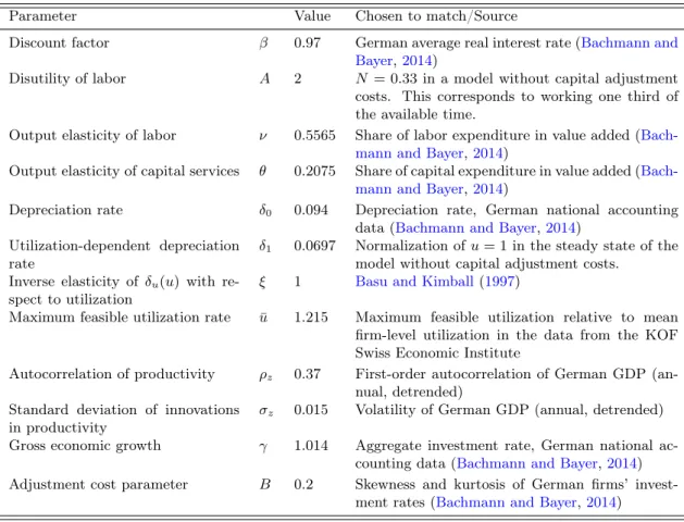
Table 4: Calibration of model parameters

Parameter Value Chosen to match/Source

Discount factor β 0.97 German average real interest rate (Bachmann and Bayer,2014)

Disutility of labor A 2 N = 0.33in a model without capital adjustment costs. This corresponds to working one third of the available time.

Output elasticity of labor ν 0.5565 Share of labor expenditure in value added ( Bach-mann and Bayer,2014)

Output elasticity of capital services θ 0.2075 Share of capital expenditure in value added ( Bach-mann and Bayer,2014)

Depreciation rate δ0 0.094 Depreciation rate, German national accounting

data (Bachmann and Bayer,2014) Utilization-dependent depreciation

rate

δ1 0.0697 Normalization ofu= 1in the steady state of the

model without capital adjustment costs. Inverse elasticity of δu(u) with

re-spect to utilization

ξ 1 Basu and Kimball(1997)

Maximum feasible utilization rate u¯ 1.215 Maximum feasible utilization relative to mean firm-level utilization in the data from the KOF Swiss Economic Institute

Autocorrelation of productivity ρz 0.37 First-order autocorrelation of German GDP (an-nual, detrended)

Standard deviation of innovations in productivity

σz 0.015 Volatility of German GDP (annual, detrended) Gross economic growth γ 1.014 Aggregate investment rate, German national

ac-counting data (Bachmann and Bayer,2014) Adjustment cost parameter B 0.2 Skewness and kurtosis of German firms’

invest-ment rates (Bachmann and Bayer,2014)

4

Model Solution

Solving for the competitive equilibrium described in the previous sections is nontrivial. The aggregate state vector includesµ, the distribution of capital across firms. This distribution is nonstandard: It has point masses because, in each period, the mass of investing firms jumps to the same point of the distribution. To address this issue, the common procedure in the lumpy investment literature consists in assuming that agents base their decisions not on the entire distribution, but only on a set of statistics or moments of the distribution.

the numerical model solution.21 However, alternative methods have been proposed to solve incomplete market models with heterogeneous agents and aggregate risk. Den Haan (2010) provides a comparison. He finds that, overall, the algorithm of Reiter (2010) performs best in terms of accuracy. In particular, this algorithm “clearly performs the best in terms of the accuracy of the individual policy rules and the accuracy of its aggregate law of motion is close to the most accurate aggregate laws of motion”. Although it is not the fastest algorithm, the method ofReiter(2010) still outperforms the Krusell-Smith algorithm in terms of speed. For these reasons, I use the method of Reiter(2010) to solve the model described in this paper.

This algorithm solves the model by backward iteration on a finite grid of points in the aggregate state space. Consistency between the solution of individual firms and the aggre-gate solution is enforced in each backward iteration step. In contrast to the Krusell-Smith algorithm, the solution method of Reiter (2010) does neither rely on a parameterization of the aggregate law of motion nor on simulations of the model. The latter might be a reason for both the better speed and the accuracy of the algorithm, as problems of sampling errors due to model simulations are avoided.

In the remainder of this section, I provide an overview of the method ofReiter(2010) and its application to the lumpy investment model with variable utilization. For more details, I refer to Reiter(2010) and the literature cited therein.

First, a grid for firm-level capital is specified. I assume that capital lies between zero and 1.15.22 100 points within this range are selected, which delivers 99 intervals over which the discrete cross-sectional distribution of capital is defined. Because there is more curvature in the region of low capital, I select smaller intervals in this part of the distribution.

Second, I compute the steady state of the model without aggregate shocks. A steady 21_{Examples includeKhan and Thomas (2003,2008), Bachmann et al. (2013) and Bachmann and Bayer} (2014). They approximate the distributionµby a finite set of its moments and its evolutionΓby a forecasting rule, usually a log-linear rule, that predicts future moments based on current moments ofµand on aggregate productivity. Moreover, a functional form for the equilibrium price is assumed. The numerical solution proceeds in two steps, which are repeated until convergence is achieved. First, conditional on the assumed pricing rule and the conjectured law of motion for the moments of the capital distribution, the dynamic programming problem becomes computable and the firms’ value and policy functions can be solved for by value function iteration. Second, given value and policy functions, the economy is simulated without imposing the presumed equilibrium pricing rule. This simulation generates time series forpand moments ofµ, which are then used to update the assumed forecasting and pricing rules. Subsequently, the procedure returns to the first step and continues until the forecasting and pricing rules converge.

22_{Zero is a natural lower bound. Larger upper bounds than 1.15 were used, but the steady state fraction} of firms with higher capital turned out to be zero. This upper bound is more than 70% larger than the steady state capital stock of 0.66. Note that, in the presence of aggregate shocks, investing firms may choose larger capital stocks than this upper bound. The value function at larger capital levels is computed using extrapolation.

state is reached if the fraction of firms lying in a specific interval of the capital distribution is constant over time, i.e., if the histogram of firm-level capital does not change over time. Solving for the steady state involves the following steps:

(1) Guess the steady state consumptionC. GivenC,pand ware determined by equations (37) and (38).

(2) Solve for the optimal firm decisions by value function iteration.23

(3) Compute the matrix of transition probabilities between the intervals of the capital dis-tribution. If p(D0) and p(D) denote next and current period’s probability distribution over firm-level capital, then the transition matrixT is characterized by

p(D0) =T p(D).

(4) Find the steady state distribution D∗ as the solution to p(D∗) =T p(D∗).

(5) Check whether the steady state distribution implies a consumption level consistent with the initial guess C. If not, restart with a different initial guess.

Third, one needs to specify a set of statistics m of the distribution µwhich replace µ as state variable. Thus, similar to the method of Krusell and Smith(1997,1998), the firms are assumed to base their decisions only on a few statistics m rather than the entire distribu-tion µ. For computational feasibility, this paper uses only the first moment of the capital distribution.24

Forth, a reference distributionDR(z, m) is specified. This is a guess of what the

distribu-tion should approximately look like if the aggregate state is (z, m). FollowingReiter (2010), I use a scaled version of the steady state distribution without shocks as reference distribu-tion. The scale factor is chosen such that the reference distribution exactly satisfies the first moment condition, i.e., EDR(z,m)[k] =m1.

Fifth, a proxy distributionDP(z, m) is chosen. This step selects the distribution that is

closest (in a mean square sense) to the reference distribution and exactly satisfies the moment conditions. Of course, this step was only necessary if m would include more than the first

23

The value and policy functions are solved for at 99 grid points corresponding to the midpointsKj of the intervals specified above.

24_{This practice is quite common in the literature.Bachmann et al.(2013) andBachmann and Bayer(2014),} for example, also rely on the aggregate capital stock only.

moment of the capital distribution because the reference distribution already exactly satisfies

EDR(z,m)[k] =m1.

Sixth, the model is solved by backward iteration. This involves the following steps: (1) Initialize next period’s value function V0(k0;z0, m0) by the steady state value function

for all z0 andm0.

(2) For any point (z, m) in the grid of aggregate states and for any value of z0, find the equilibrium values ofm0. This requires the following substeps:

(2.1) Guessm0 and p. Given p,w is determined by equation (38).

(2.2) Use an interpolation scheme to obtain the value function off the grid form0. I use the shape-preserving quadratic spline of Schumaker(1983) (see also Judd, 1998). This method also provides an algorithm to obtain estimates of the slope of the value function.

(2.3) Compute optimal labor, utilization and capital choices of investing firms starting from the proxy distribution DP(z, m). Equations (39) and (40) yield the

closed-form solution for nf_I and uI as a function ofk,z and w. Given V0 and the guess

for p, (24) determines the optimal capital choicek0.25

(2.4) Compute optimal labor and utilization choices of non-investing firms starting from the proxy distribution DP(z, m). Computations are more involved than for

in-vesting firms. An essential element that speeds up the solution is the use of the endogenous grid point method of Carroll(2006). The basic idea is to formulate a grid for k0 rather than k. Let K_j, j = 1, . . . , nk, denote the grid points for

firm-level capital. Using the firms’ optimality conditions, one can deduce the capital levelsk˜j at which it is optimal to choose a capacity utilization leading tok0j =Kj.

The value function at the endogenous grid points ˜kj can then be computed

with-out actually solving a maximization problem because the grid points are chosen such that k_j0 =Kj is the optimal outcome. Finally, Schumaker splines are used to

obtain the value of non-investing firms at the grid points of the proxy distribution instead of ˜kj.

25_{The next period’s value functionV}0

is known from the previous backward iteration step or, in the first iteration, from the steady state.

(2.5) Substeps (2.3) and (2.4) yield the value of investment and non-investment at the grid points of the proxy distribution. Equation (30) then determines the threshold for the binary investment decision at each of these grid points.

(2.6) Compute aggregate variables. Check whether the resultingpandm0 are consistent with the guess from substep (2.1). If not, restart with a different initial guess. (2.7) From the previous substeps, the value V˜(k;z, m, z0, m0(z, m, z0)) is obtained at

each grid point forkof the proxy distribution. Schumaker splines are then used to compute the value at the original grid pointsK_j.

(3) Update the value function usingV˜(k;z, m, z0, m0(z, m, z0))from the previous step. For each Kh,zand m, the updated value function is given by

V(Kh;z=zi, m) =

X

j

πjiV˜(Kh;z=zi, m, z0=zj, m0(zi, m, z0 =zj)). (44)

Steps (2) and (3) of this backward iteration are repeated until convergence in the value function is achieved. I use the criterion that the absolute difference between the value functions of two consecutive iterations is at most 10−6 _{for all grid points.}

As pointed out by Reiter (2010), computation can be accelerated by not solving for

m0(z, m, z0) in every iteration. After some full iterations consisting of steps (2) and (3),

m0(z, m, z0) is only computed every few iterations with some intermediate “acceleration

iter-ations” which use m0(z, m, z0) of the previous full iteration.

5

Results

This section presents the results from the lumpy investment model with variable capacity utilization, starting with a description of the steady state, followed by a characterization of optimal firm-level decisions on investment, utilization and labor, and closing with a description of the macroeconomic implications thereof. The results of this paper’s model are compared with those of three other models which differ in either or both of the following two dimensions: whether utilization is variable and whether capital adjustment entails fixed costs. Thus, four models are compared: this paper’svariable utilization lumpy investment model (VULIM), the standard lumpy investment model (SLIM) with fixed utilization, a variable utilization fric-tionless model (VUFM) without fixed capital adjustment costs, and the standard frictionless