Dynamic Price Competition
with Price Adjustment Costs
and Product Differentiation
Gianluigi Vernasca
NOTA DI LAVORO 120.2003
DECEMBER 2003
CTN – Coalition Theory Network
Gianluigi Vernasca, Department of Economics, University of Warwick
This paper can be downloaded without charge at: The Fondazione Eni Enrico Mattei Note di Lavoro Series Index: http://www.feem.it/Feem/Pub/Publications/WPapers/default.htm Social Science Research Network Electronic Paper Collection:
http://papers.ssrn.com/abstract_id=XXXXXX
The opinions expressed in this paper do not necessarily reflect the position of Fondazione Eni Enrico Mattei
Dynamic Price Competition with Price Adjustment Costs and Product
Differentiation
Summary
We study a discrete time dynamic game of price competition with spatially differentiated products and price adjustment costs. We characterise the Markov perfect and the open-loop equilibrium of our game. We find that in the steady state Markov perfect equilibrium, given the presence of adjustment costs, equilibrium prices are always higher than prices at the repeated static Nash solution, even though, adjustment costs are not paid in steady state. This is due to intertemporal strategic complementarity in the strategies of the firms and from the fact that the cost of adjusting prices adds credibility to high price equilibrium strategies. On the other hand, the stationary open-loop equilibrium coincides always with the static solution. Furthermore, in contrast to continuous time games, we show that the stationary Markov perfect equilibrium converges to the static Nash equilibrium when adjustment costs tend to zero. Moreover, we obtain the same convergence result when adjustment costs tend to infinity.
Keywords: Price adjustment costs, Difference game, Markov perfect equilibrium, Open-loop equilibrium
JEL: C72, C73, L13
I would like to thank Myrna Wooders for her valuable comments and suggestions. I wish also to thank Paolo Bertoletti, Jonathan Cave, Javier Fronti, Augusto Schianchi for useful conversations, and the participants of seminars at the University of Warwick, the University of Pavia and at the EARIE 2003 Conference in Helsinki. Any mistakes remain my own.
Address for correspondence:
Gianluigi Vernasca Department of Economics University of Warwick Coventry CV4 7AL United Kingdom Phone: + 44 (0) 247652 23479 Fax: + 44 (0) 247652 3032 E-mail: G.Vernasca@warwick.ac.uk
1
Introduction
In this paper we develop a duopolistic dynamic game of price competition, in which products are horizontally di¤erentiated and …rms face adjustment costs every time they change their prices. Imposing adjustment costs creates a time dependent struc-ture in our dynamic game and allows us to develop our model as a discrete time
di¤erential game, or di¤erence game.1 The main objective of our analysis is to study
the e¤ects of the presence of such adjustment costs on the strategic behaviour of …rms under di¤erent assumptions on the ability of the …rms to commit to price paths in advance. In particular, we focus on two di¤erent classes of strategies that have been widely used in the dynamic competition models, Markov and open-loop
strate-gies.2 Markov strategies depend only on payo¤ relevant variables that condense the
direct e¤ect of the past on the current payo¤.3 The use of Markov strategies restrict
equilibrium evaluation solely to subgame perfect equilibria, which have the desirable property of excluding non-credible threats. In contrast, open-loop strategies are func-tions of the initial state of the game and of the calendar time, and typically, are not subgame perfect. Thus, Markov and open-loop strategies correspond to extreme as-sumptions about player’s capacities to make commitments about their future actions. Under the open-loop information pattern, the period of commitment is the same as the planning horizon while under Markovian strategies no commitment is possible.
The role of price stickiness has been analysed in many theoretical models of
busi-ness cycles.4 Very little attention, however, has been paid to strategic incentives
associated with price adjustment costs in dynamic oligopoly models. There are
sev-1Di¤erential games are dynamic games in continuous time, in which the di¤erent stages of the
game are linked through a transition equation that describes the evolution of the state of the model. Furthermore, the transition equation depends on the strategic behaviour of the players. These kind of games are also called “state-space” games. Di¤erence games are the discrete time counterpart of di¤erential games. See Basar and Olsder (1995) for a detailed analysis. See also De Zeeuw and Van Der Ploeg (1991) for a survey on the use of di¤erence games in economics.
2See Fudenberg and Tirole (1991) Ch. 13, for and introduction to Markov and open-loop
equi-libria and on their use in dynamic games. Amir (2001) provides an extensive survey on the use of these strategies in dynamic economic models.
3There is no generally accepted name in di¤erence/di¤erential games theory for such strategies
and for the related equilibrium. Basar and Oldser (1995) use the term “Feedback Nash rium” while Papavassilopoulos and Cruz (1979) use the term “Closed-Loop Memoryless Equilib-rium”. However, after Maskin and Tirole (1988), the terms Markov strategies and Markov Perfect equilibrium has become standard in economic literature.
4Two di¤erent possibilities to model price adjustment costs have been considered in the literature
on business cycles. First, there is a …xed cost per price change due to the physical cost of changing posted prices. These …xed costs are called ”menu costs”. See for example, Akerlof and Yellen (1985) and Mankiw (1985) among the others. Second, there are costs that capture the negative e¤ect of price changes, particularly price increases on the reputation of …rms. These costs are quadratic because reputation of …rms is presumebly more a¤ected by large price changes than by small price changes. See for example, Rotemberg (1982). In our model, we follow the latter approach.
eral examples of di¤erential games of Cournot competition with sticky prices, like Fershtman and Kamien (1987), Piga (2000) and Cellini and Lambertini (2001.a). The main result of these authors is that the subgame perfect equilibrium quantity is always below the static Cournot equilibrium, even if prices adjust instantaneously. This implies that the presence of price rigidity creates a more competitive market outcome. However, in those models, price rigidity is not modelled using adjustment costs, but instead refers to stickiness in the general price level. Thus those models deal only with one state variable, that is, the price level given by the inverse de-mand function, while in our model we have two state variables, the two prices of both …rms. This fact adds considerably to the technical complexity of our problem. The main reason is that dynamic programming su¤ers the “curse of dimensional-ity”, that is the tendency of the state space, and thus computational di¢ culties, to grow exponentially with the number of state variables. As far as adjustment costs are concerned, most of the literature on dynamic competition has instead focused on adjustment costs in quantities. However, the same result described above still hold when these adjustment costs are considered. For example, Reynolds (1989, 1991) and Driskill and McCa¤erty (1989) study a dynamic duopoly with homogenous products and quadratic capacity adjustment costs in continuous time setting. The steady state output in the subgame perfect equilibrium is found to be larger than in the Cournot static game without adjustment costs. The main reason is the presence of intertempo-ral strategic substitutability in the strategic behaviour of the …rms. A larger output of a …rm today leads the …rm being more aggressive tomorrow. The same result seems to hold independently on the kind of competition that is considered, as showed by Jun and Vives (2001) in their model of Bertrand competition with output adjustment costs.5
All the literature described so far shares the common feature of a continuous time setting. An interesting limit result that is common to models of dynamic oligopoly in continuous time is that, as adjustment costs or price stickiness tend to zero, the subgame perfect equilibrium approaches a limit that is di¤erent from the Nash equi-librium of the corresponding static game. Discrete time models of dynamic compe-tition have been less developed, since it appears that the discrete time formulation is less tractable than the continuous time formulation. Discrete time models of dy-namic competition with adjustment costs have been analysed in Maskin and Tirole (1987), Karp and Perlo¤ (1993) and Lapham and Ware (1994) among others. In the …rst case Cournot competition with quantities adjustment costs is considered, but the equilibrium has been characterised only for the case in which adjustment costs approach in…nity. More interesting for our purposes is the model of Lapham and Ware (1994). They show that the taxonomy of strategic incentives developed by Fu-denberg and Tirole (1984) in a two-stage game can be extended to in…nite horizon games with Markov strategies. However, their analysis is limited to the case in which
5This seems to provide a counterpoint to the idea of Kreps and Scheinkman (1983) that quantity
adjustment costs are zero in equilibrium. Nevertheless, they …nd a limit result that contradicts the one of continuous time models. When adjustment costs tend to zero, their steady-state Markov perfect equilibrium converges to the Nash equilibrium of the static game.
In our model we characterize the Markov perfect equilibrium for di¤erent values of adjustment costs and product di¤erentiation. Given the mathematical complexity involved in the analysis, some qualitative results are derived with numerical simu-lation. We …nd that the prices at the steady-state Markov perfect equilibrium are always higher than the prices at the static Nash equilibrium of the corresponding static game but they coincide in two limit cases – when adjustment costs tend to zero and when they tend to in…nity. The economic force behind this result is the presence of intertemporal strategic complementarity: a …rm, may strategically raise price today, and induce high prices from its rival tomorrow. The presence of ad-justment costs enables …rms to increase prices today and signal that they plan to keep prices higher next period. However, the magnitude of this strategic comple-mentarity depends on the level of product di¤erentiation. As products become less di¤erentiated, higher equilibrium prices are sustainable only if adjustment costs are su¢ ciently high. Strategic complementarity is absent in open-loop strategies and the steady-state open-loop equilibrium is in correspondence one-to-one with the static Nash equilibrium. Our analysis is conducted under the assumptions that demand functions are linear function of prices and that pro…t functions and adjustment costs are quadratic and symmetric between …rms. With this structure our model is a linear quadratic game. This kind of game is analytically convenient because the equilibrium strategies are known to be linear in the state variables of the model. Moreover, in some cases linear quadratic models or linear quadratic approximations of non-linear games provide a good representation of oligopolistic behaviour especially around a deterministic steady state.
The paper is organized as follows. In section 2 we describe the model. Section 3 presents the full computation of the Markov perfect equilibrium. In Section 4 we compare the Markov perfect equilibrium with the open-loop equilibrium and then we consider some limit results for these two equilibria. Section 5 concludes.
2
The Model
We start with the derivation of the demand functions. Consider a simple model
of spatial competition a’ la Hotelling in which there is a continuum of consumers
uniformly distributed in the unit interval[0;1];with the position of a …rm representing its ideal product. Consumers incur exogenous ‘transportation costs’ for having to consume one of the available brands instead of their ideal brand. This cost has the form of(1=2s), wheres2(0;1]provides a measure of substitutability between both
products.6 In particular, when the transportation cost tends to zero, products become
close substitutes. In contrast, if1=2s! 1 , a consumer prefers to choose the brand
closest to its ideal point, independent of price. Thus, we can think atsas an indicator
of market power of …rms. Indeed, when products are highly di¤erentiated (sis small),
…rms can increase prices without signi…cantly a¤ecting their own demand.
The utility function at time t of the consumer located at point in the unit
seg-ment, for product i, is a linear functionUt(v; i; s; pit) = v j i Fij
2s pit: The termv
represents the utility that a consumer derives for consuming her ideal product, that
is assumed to be time invariant. Given our speci…cation, the term v represents also
an upper boundary level for the price set.7 If prices plus the exogenous
transporta-tion costs are greater thanv, then no products will be bought by the consumers. In
the following we shall assume that v is su¢ ciently high so that this does not occur.
Finally,Fi 2[0;1]is the location of …rmi;and the term pitre‡ects the negative
im-pact of price of production the utility of consumers. Following standard procedures,
we solve for the demand functions of a consumer ewho is at the point of indi¤erence.
The linear demand function faced by …rm iis simply
yit(pit; pjt) = 1
2 +s(pjt pit) (1)
with i; j = 0;1 and i6=j: If …rms set the same price, both share equally the market.
In our duopoly model the two …rms are symmetric and they are located at each end of the unit interval. There is no uncertainty. Both …rms face …xed quadratic adjustment costs: 12 (pit pit 1)
2
;where 0is a measure of the cost of adjusting
the price level.8 This formulation implies that adjustment costs are minimized when
no adjustment takes place. The per-period pro…t function for …rm i is the following
concave function in its own prices:
it(pit; pjt; pit 1) = pityit(pit; pjt) 1
2 (pit pit 1)
2
(2)
At time t; …rm i decides by how much to change its price it = (pit pit 1), or
equivalently to set the new price level at time t: Thus, using the terminology of the
optimal control theory, prices at time t are the control variables for the …rms, while
prices at timet 1 are the state variables.
Firmimaximizes the following discounted stream of future pro…ts over an in…nite
horizon:
6The formulation of the consumer problem is standard and follows the lines as in Doganouglu
(1999). Di¤erently from his analysis, we do not incorporate possible persistent e¤ects in customer tastes.
7The fact that the set of prices is bounded assures that instantaneous pro…t functions are bounded
as well, which is a su¢ cient condition for dynamic programming to be applicable. See Maskin and Tirole (1988.b).
8We use convex adjustment costs as in Rotemberg (1982). Quadratic price adjustment costs have
been used also by Lapham and Ware (1994) and Jun and Vives (2001) because of their analytical tractability.
i = 1 X t=1 t it(pit; pjt; pit 1) (3)
where 2(0;1)is the time invariant discount factor.9
With this structure, our model is a linear quadratic game. This kind of games is analytically convenient because the equilibrium strategies are known to be linear in the state variables.10
In our model, we mainly focus on strategic behaviour of the …rms based on pure Markov strategies, that is, Markov strategies that are deterministic, in which the past in‡uences current play only through its e¤ect on the current state variables that summarise the direct e¤ect of the past on the current environment. Optimal Markovian strategies have the property that, whatever the initial state and time are, all remaining decisions from that particular initial state and particular time onwards must also constitute optimal strategies. This means that Markov strategies are time-consistent. An equilibrium in Markov strategies is a subgame perfect equilibrium and it is called Markov perfect equilibrium11.
Following Maskin and Tirole (1988), we de…ne a Markov perfect equilibrium using
the game theoretic analogue of dynamic programming12:
De…nition 1 . LetVit(pit 1; pjt 1), withi; j=1,2 andi6=j;be the value of the game
starting at period t where both players play their optimal strategy (peit(pit 1; pjt 1) for
i; j=1,2 and i 6= j). This pair of strategies constitute a Markov Perfect Equilibrium (MPE) if and only if they solve the following dynamic programming problem:
Vit(pit 1; pjt 1) = M ax
pit
[ it(pit; pjt; pit 1)) + Vit+1(pit; pjt)] (4)
The pair of equations in 4) are the Bellman’s equations of our problem that have to hold in equilibrium. Di¤erentiating the right-hand side of the Bellman’s equations 4) with respect the control variable of each …rm, we obtain the following …rst order conditions:
9The presence of a discount factor less than one together with per-period payo¤ functions
uni-formly bounded assures that the objective functions faced by players are continuous at in…nity. Under this condition a Markov perfect equilibrium, at least in mixed strategies, always exist in a game with in…nite horizon. See Fudenberg and Tirole p. 515.
10For a detailed analysis of this point, see Papavassilopoulos, Medanic and Cruz (1979)
11The concept of subgame perfection is much stronger than time consistency, since it requires that
the property of subgame perfection hold at every subgame, not just those along the equilibrium path. On the other hand, dynamic (or ”time”) consistency would require that along the equilibrium path the continuation of the Nash equilibrium strategies remains a Nash equilibrium. For a discussion on the di¤erence between subgame perfection and time consistency see Reinganum and Stokey (1985).
12By de…nition, Markov strategies are feedback rules. Furthermore, it is well known that dynamic
programming produces feedback equilibria by its very construction , thus, it represents a natural tool to analyse Markov perfect equilibria.
@ it(pit; pjt; pit 1)
@pit
+ @Vit+1(pit; pjt)
@pit
= 0 (5)
Given the linear quadratic nature, the …rst order conditions of each player com-pletely characterize the Markov perfect equilibrium. To solve this system of equations,
we need to guess a functional form for the unknown value functions Vi( ): However,
we know that equilibrium strategies in linear quadratic games are linear functions of the state variables and value functions are quadratic. Then, we guess the following functional form for the value functions:13
Vit+1(pit; pjt) = ai+bipit+cipjt+
di 2p
2
it+eipitpjt+fip2jt for i; j = 1;2 and i6=j (6)
where the parameters ai; bi; ci; di; ei and fi are unknown parameters. Equation 6)
hold for everyt:
We are not interested in solving for all these parameters since we are analysing only the derivatives of the value functions that are given by:
@Vit+1(pit; pjt) @pit =bi+dipit+eipjt for i; j = 1;2and i6=j (7.1) @Vit+1(pit; pjt) @pjt =ci+eipit+fipjt for i; j = 1;2 and i6=j (7.2)
where the coe¢ cients bi; ci; di; ei and fi are the parameters of interest that are to be
determined by the method of undetermined coe¢ cients (See Appendix). A solution for those coe¢ cients, if it exists, will be a function of the structural parameters of
the model given by s; and : Substituting the relevant derivatives of the payo¤
functions and equations 7.1) and 7.2) into 5), we can obtain a solution for the current prices (pit; pjt) as a linear function of the state variables (pit 1; pjt 1). This solution
is given by the following pair of linear Markov strategies:
e
pit =Fi+Ripjt 1+Mipit 1 for i; j = 1;2 and i6=j (8)
where the coe¢ cients Fi; Ri andMi are functions directly and indirectly, through
the unknown parameters of the derivatives given by 7.1) and 7.2), of the structural
parameters of the model (s; and ): (See Appendix).
We can substitute optimal strategies given by 8), after taking into account for symmetry, into the Bellman’s equations 4), and then di¤erentiating 4) for the state
variables (pjt 1; pit 1 ). Using the …rst order conditions 5) to apply the Envelope
theorem, we obtain the following system of four Euler equations:
13Since the mathematical analysis involved is standard, we follow the same procedure as in Lapham
@Vit @pit 1 = @ it @pit 1 + @ it @pejt + @Vit+1 @pejt @pejt @pit 1 for i; j = 1;2 and i6=j (9.1) @Vit @pjt 1 = @ it @pjt 1 + @ it @epjt + @Vit+1 @pejt @epjt @pjt 1 for i; j = 1;2and i6=j (9.2)
where the pro…t functions are given by it(epit(pit 1; pjt 1);pejt(pit 1; pjt 1); pit 1):
Using equations 7.1) and 7.2) in the above Euler equations, and using the method of undetermined coe¢ cients, we obtain ten non-linear equations in ten unknowns parameters ai; bi; ci; di; ei and fi for i = 1;2 (system A3) in the Appendix): If a
solution for these parameters exists, then the linear Markov perfect equilibrium given by 8) exists as well. Given the fact that we have to deal with ten non-linear equations, to simplify the mathematical tractability of the model, we restrict our analysis to a
symmetric Markov perfect equilibrium.14 This implies that from equations 7.1) and
7.2) we have b1 = b2 = b; c1 = c2 =c; d1 = d2 = d; e1 = e2 = e and f1 = f2 = f:
Thus, Markov strategies are also symmetric, that is, F1 = F2 = F; R1 = R2 = R
and M1 = M2 = M: Suppose that a solution for the unknown parameters exists,
and denote this solution with b ; c ; d ; e and f : Using symmetry in the Markov
strategies, and using the de…nitions given in the Appendix for the coe¢ cients F; R
and M, we can solve for the symmetric steady state level of the system of …rst order
di¤erence equations given by 8): pmpei = 1
2
1 + 2 b
s (d +e ) fori= 1;2 (10)
where we assume s6= (d +e ). The equilibrium in 10) is the steady-state linear
Markov perfect equilibrium of our model. Note that when s tends to in…nity the
equilibrium prices tend to zero. In the next section we will show how to derive a
solution for the unknown parameters b ; c ; d ; e and f . Then, we will consider in
details the properties that the equilibrium given by 10) exhibits.
3
Computation and Properties of the Markov
Per-fect Equilibrium
In this section we compute more in detail the linear Markov perfect equilibrium of our model. We start with the derivation of the Nash equilibrium of the static game
14Strategic symmetric behaviour by …rms is a standard assumption in the literature on dynamic
competition. See for example, Jun and Vives (2001), Driskill and McA¤erty (1989) and Doganouglu (1999) among the others. This assumption can be seen as a natural consequence of the fact that …rms face a symmetric dynamic problem. However, we are aware that the presence of ten non-linear equations implies that many equilibria, symmetric and not, can arise from our model.
associated with our model without adjustment costs.15 This particular equilibrium represents a useful benchmark that can be compared with the Markov perfect and the open-loop equilibria of the model and it will be useful when will study the convergence
properties of such equilibria when adjustment costs tend to zero. Assuming = 0;
the symmetric static equilibrium of the repeated game without adjustment costs, denoted by ps; is given by:
ps = 1
2s (11)
As we might expect, without adjustment costs, prices in equilibrium are functions of the measure of substitutability between the two goods. As for the Markov
per-fect equilibrium, when goods are perper-fectly homogeneous (s tends to in…nity) static
equilibrium prices are zero as in the classical Bertrand model.
In order to derive the properties of the Markov perfect equilibrium given by 10) we
need to …nd a solution for the parameters of the value functionsb ; c ; d ; e and f :
Despite the tractability of linear quadratic games, given the analytical di¢ culty to deal with a highly non-linear system of implicit functions, most of the results that we
are going to present are obtained using numerical methods.16 Numerical techniques
are often used in dynamic games in state-space form, as in Judd (1990) or Karp and Perlo¤ (1993). The presence of nonlinearity implies that we must expect many
so-lutions for the unknown parameters, and thus, multiple Markov perfect equilibiria.17
In order to reduce this multiplicity, we concentrate our analysis to symmetric Markov perfect equilibria that are asymptotically stable as in Driskill and McCa¤erty (1989) and Jun and Vives (2001). An asymptotically stable equilibrium is one where the equilibrium prices converge to a …nite stationary level for every feasible initial
condi-tion.18 The symmetric optimal Markov strategies are given by:
e
pit =F +Rpjt 1+M pit 1 for i; j = 1;2and i6=j (12)
From these strategies we can derive the conditions for stability of the symmetric linear Markov perfect equilibrium:
Proposition 1 Assuming in 12) that (2s+ d) 6= (s+ e); then, this pair of strategies de…nes a stable equilibrium, if and only if, the eigenvalues of the symmetric
15This particular equilibrium is important because it represents a subgame perfect equilibrium of
the in…nite repeated game without adjustment costs associated with our model.
16In particular, we use the Newton’s method for nonlinear systems. For an introduction to the
Newton’s method, see Cheney and Kincaid (1999), Ch.3.
17Unfortunately, in literature, there are no general results on the uniqueness of Markov perfect
equilibria in dynamic games. An interesting exception is Lokwood (1996) that provides su¢ cient conditions for uniqueness of Markov perfect equilibria in a¢ ne-quadratic di¤erential games with one state variable.
18Given the lack of a transversality condition in the dynamic problem stated in De…nition 1, we
focus on asymptotically stable equilibria also because in this case we know that these equilibria will ful…l the tranversality condition even implicitly.
matrix A= M R
R M are in module less than one. This implies that conditions for the stability of the system given by 12) are: (d e)< 3s and (d+e)< s:
The result in Proposition 1 is derived from the theory of dynamic systems in
discrete time.19 The condition that(2s+ d)
6
= (s+ e)assures that the parameters
of the Markov strategies 12) are well de…ned (see Appendix). Thus, when we look for a solution of the system A3) de…ned in the Appendix, this solution should respect the conditions in Proposition 1. Moreover, we consider only real solutions for the unknown parameters, and we consider only solutions that are locally isolated, or
locally stable.20 In addition, we impose that at that solution, equilibrium prices
cannot be negative. Thus, we construct an asymptotically stable Markov perfect equilibrium numerically, instead of analytically as in Drisckill and McCa¤erty (1989) and Jun and Vives (2001).
We now focus on the properties of our Markov perfect equilibrium when adjust-ment costs are positive and …nite. We solve the system A3) in the Appendix for
given values of the transportation cost (s), the discount factor ( ); and the measure
of adjustment costs ( ):21 Given the stability conditions stated above, we obtain a
unique solution for the parametersb; c; d; eand f and thus, a unique Markov perfect
equilibrium, for each set of values of the structural parameters of the model (s; and
)22: Given the di¢ cult economic interpretation for these parameters, a sample of
results is given in the Appendix. Here we report the implications of those solutions
for the coe¢ cients of the symmetric Markov strategiesF; M andR:We are interested
in particular on the coe¢ cientR that represents the e¤ect of one …rm’s today choice
on the rival’s choice tomorrow.
Proposition 2 For a plausible range of the structural parameters of the model s; and , we have the following results at the stable solutions of the system A3):
1) the coe¢ cients of the Markov strategies are always positive;
2) R is …rst increasing and then decreasing in : The higher s the higher is the persistence of the increasing phase;
3) R is decreasing in s when adjustment costs are small. When adjustment costs become higher, R …rst increases and then decreases in s: The higher ; the higher is the persistence of the increasung phase.
19Drisckill and McCa¤erty (1989) and Jun and Vives (2001) construct an asymptotically stable
Markov equilibrium using similar conditions for di¤erential equations, called Routh-Hurwitz condi-tions. For the case of a2 2system of di¤erence equations, these conditions imply thatjdet(A)j<1
andjdet(A) + 1j< tr(A);wheretr is the trace of matrix A.
20In practice, we want that at one particular solution, if we perturb that solution, the system of
implicit functions A3) must remain close to zero.
21Most of our results are based on a value of close to 1, a value that we take from the numerical
analysis of Karp and Perlo¤ (1993).
22Driskill and McCa¤erty (1989) and Jun and Vives (2001), using a similar framework as ours, have
4) we have always M > R, however, the di¤erence (M R) is decreasing in s;
5) the coe¢ cient M is increasing in and decreasing in s;
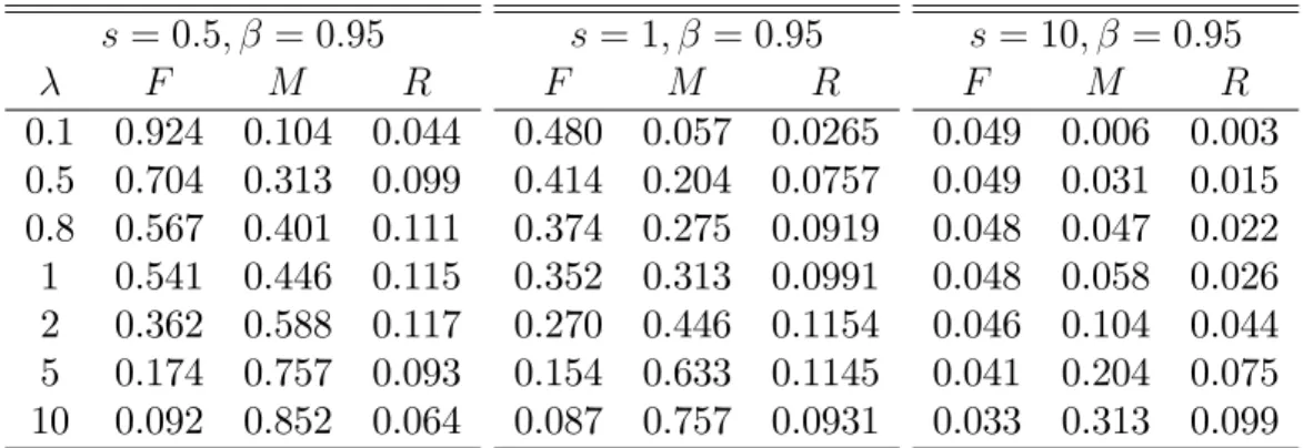
The statements in Proposition 2 are summarised in the following table, in which we report a sample of the results of our numerical analysis made on system A3.
Table 1. Numerical values for the coe¢ cients of Markov strategies. s = 0:5; = 0:95 F M R 0.1 0.924 0.104 0.044 0.5 0.704 0.313 0.099 0.8 0.567 0.401 0.111 1 0.541 0.446 0.115 2 0.362 0.588 0.117 5 0.174 0.757 0.093 10 0.092 0.852 0.064 s = 1; = 0:95 F M R 0.480 0.057 0.0265 0.414 0.204 0.0757 0.374 0.275 0.0919 0.352 0.313 0.0991 0.270 0.446 0.1154 0.154 0.633 0.1145 0.087 0.757 0.0931 s= 10; = 0:95 F M R 0.049 0.006 0.003 0.049 0.031 0.015 0.048 0.047 0.022 0.048 0.058 0.026 0.046 0.104 0.044 0.041 0.204 0.075 0.033 0.313 0.099
In Proposition 2, we have identi…ed the strategic behaviour of …rms when adjust-ment costs are positive and …nite. Not surprisingly, we have that the optimal price choice of a …rm is an increasing function in the rival’s price and this e¤ect is captured
by the coe¢ cientR: Thus, the strategic behaviour of the …rms in our model, is
char-acterised by intertemporal strategic complementarity. Furthermore, the size of the
e¤ect of strategic complementarity as a function of follows a bell-shaped curve. For
small adjustment costs, it increases, while, when adjustment costs become higher, it
decreases until it reaches zero as approaches in…nity. However, results 2) and 3) in
the above Proposition say that this relationship depends on the measure of product
di¤erentiation s: When s is high, competition between …rms becomes …ercer, since
small changes in prices can have huge e¤ects on consumer’s demand. In this case, to sustain a credible strategy of increasing prices it is necessary to have a relatively
higher level of adjustment costs than in the case in which s is small and …rms have
higher market power. Finally, result 4) in Proposition 2) says that as s increases,
…rms tend to assign a relatively higher weight to the rival’s price in their strategic behaviour than in the case in which products are more di¤erentiated. From Propo-sition 2, we can identify the e¤ects of positive adjustment costs on the steady-state Markov perfect equilibrium of our model. The main result is stated in the following Proposition:
Proposition 3 When adjustment costs are positive and …nite, prices at the sym-metric steady state Markov perfect equilibrium are always higher than prices in the equilibrium of the repeated static game. This is true, even though, no adjustment costs are paid in the steady state.
The equilibrium values of the Markov perfect and the corresponding static Nash equilibrium for the same sample used in Table 1 are reported in the following table.
Table 2. Comparison between the symmetric Markov perfect and the counterpart static Nash equilibrium.
s= 0:5; = 0:95 pmpe ps 0.1 1.086 1 0.5 1.199 1 0.8 1.225 1 1 1.234 1 2 1.233 1 5 1.168 1 10 1.106 1 s= 1; = 0:95 pmpe ps 0.525 0.5 0.575 0.5 0.592 0.5 0.599 0.5 0.615 0.5 0.609 0.5 0.582 0.5 s= 10; = 0:95 pmpe ps 0.0503 0.05 0.0513 0.05 0.0521 0.05 0.0525 0.05 0.0543 0.05 0.0570 0.05 0.0573 0.05
From Proposition 3 we can say that in our dynamic game, the presence of adjust-ment costs and the hypothesis of Markov strategies create a strategic incentive for the …rms to deviate from the equilibrium of the repeated static game even if adjustment costs are not paid in steady state. The result is a less competitive behaviour by the …rms in the Markov equilibrium than in the static case. The economic force behind this result is the presence of intertemporal strategic complementarity that we have analysed above. A …rm by pricing high today will induce high prices from the rival tomorrow, and the cost of adjusting prices lends credibility to this strategy, since it is costly to deviate from that strategy. The result in Proposition 3) contrasts with the one found in dynamic competition models with sticky prices, where general price stickiness creates a more competitive outcome in the subgame perfect equilibrium than in the static Nash equilibrium. The main reason is that in our model, price rigidity is modelled directly in the cost functions of the …rms and there is a credi-bility e¤ect associated with adjustment costs that can sustain high equilibrium price strategies, while, this credibility e¤ect is absent with general price stickiness. We
can notice that as products become close substitutes (s increases), the higher is the
level of adjustment costs the higher is the di¤erence between pmpeand psrelatively
to the case where s is small. The intuition is the same as the one described above
to explain results 2) and 3) of Proposition 2). When s is high, …rms have a strong
incentive to reduce their prices of a small amount in order to capture additional de-mand. Large adjustment costs can o¤set this incentive because the credibility of a high price equilibrium strategy will be stronger. Obviously, we know already from Proposition 2) that this credibility e¤ect is not increasing monotonically with ,
be-cause as adjustment costs become extremely high, the coe¢ cientR tends to zero. We
shall analyse this aspect in more detail when we will consider the properties of the Markov perfect equilibrium in the limit game. The result in Proposition 3) states that when adjustment costs are positive, …rms are better o¤ in the steady state Markov perfect equilibrium than in the static Nash equilibrium of the repeated game. Thus, the presence of positive adjustment costs can induce a tacit collusive behaviour by
products are perfect substitute, we already know that the Markov perfect equilibrium
given by 10) converges to the static Nash equilibrium independently of the value of :
Moreover, in this case, both equilibria are equal to zero and we fall into the classical ”Bertrand paradox”.
3.1
Markov Perfect Equilibrium in the Limit Game
We now consider the properties of the Markov perfect equilibrium of our model in di¤erent limit cases. Di¤erently from previous section, the results we are going to show are obtained analytically. We start our analysis evaluating the steady state Markov perfect equilibrium given by 10) in two limit cases, when adjustment costs
tend to zero ( ! 0); and when they are in…nite ( ! 1): This allows us to de…ne
the convergence properties of the steady-state Markov perfect equilibrium given by 10) toward the static Nash equilibrium 11), that, as we know from the introduction, is an important issue for the literature on dynamic competition. In order to describe the behaviour of the equilibrium in 10) in the two limit games, we need to evaluate the system A3) in the Appendix in the two extreme assumptions on the adjustment
costs parameter : The results for our limit games are the following:
Proposition 4 When adjustment costs tends to zero ( !0);the symmetric solution for the unknown parameters is the following: b = c = d = e = f = 0; and the steady-state Markov perfect equilibrium corresponds with the static Nash equilibrium of the repeated game. When adjustment costs tend to in…nity ( ! 1), the symmetric solution for the unknown parameters is: b = 1
2; c= 0; d = 2s; e =s; f = 0;and
the steady-state Markov perfect equilibrium converges to the static Nash equilibrium given by 10).
Proof (see Appendix). The convergence of the steady state Markov perfect equilib-rium toward the static Nash equilibequilib-rium when adjustment costs tend to zero con…rms the result found in Lapham and Ware (1994), and it contradicts the results found in continuous time models of dynamic competition. In our discrete time model, as in Lapham and Ware (1994), the discontinuity found in continuous time models, when adjustment costs tend to zero, disappears. This result is supported by the numerical analysis developed by Karp and Perlo¤ (1993), that gives also a possible explana-tion of why discrete and continuous time behave di¤erently in the limit case of zero adjustment costs. In their model, they show that the steady-state Markov perfect
equilibrium becomes more sensitive to when we pass from discrete time to
continu-ous time. On the other hand, the second result is common in discrete and continucontinu-ous time models, like in Maskin and Tirole (1987) and Reynolds (1991). The economic intuition behind this result is that: when adjustment costs become very large, the extra costs to change prices strategically outweight the bene…ts, thus, …rms are in-duced to behave nonstrategically and the steady-state subgame perfect equilibrium converges to the static solution. Of course, the case with in…nite adjustment costs
is not very practical, especially for our purpose, since we are dealing with price
ad-justment costs that are normally associated with a small value of : However, this
limit result is important because it shows that our value functions are continuous
at in…nity23. Finally, we consider what happens to the steady state Markov perfect
equilibrium when tends to zero, that is, when only present matters for …rms.
Fer-shtman and Kamien (1987), using a continuous time model with sticky prices, found that when only present matters for …rms their stationary Markov perfect equilibrium converges to the competitive outcome. On the other hand, Driskill and McCa¤erty (1989), using a similar model but with adjustment costs in quantities, found that the Markov perfect equilibrium converges to the static Nash equilibrium of the repeated game without adjustment costs. In our model, we have the following result:
Proposition 5 As ; the discount factor, tends to zero, the steady state Markov perfect equilibrium given by 10) tends to the static Nash equilibrium of the repeated game without adjustment costs.
The proof of this Proposition can be easily seen taking the limit of the Markov
perfect equilibrium in 10) for !0: In this case, it is simple to see that the result is
the static Nash equilibrium given by 11).
As we might expect, if future does not matter for …rms, the result is the equilibrium of the one shot game. We obtain a result similar to the one of Driskill and McCa¤erty (1989), however, if we allow products to be homogeneous our equilibrium converges to the competitive outcome as in Fershtman and Kamien (1989), that, in our case, implies equilibrium prices equal to zero.
4
The Open-Loop Equilibrium
In this section we will analyse what are the e¤ects of adjustment costs on equilibrium price if we force …rms to behave using open-loop strategies. While Markov strate-gies are feedback rules, open-loop stratestrate-gies are trajectory, or path, stratestrate-gies. In particular, open-loop strategies are functions of the initial state of the game (that is known a priori) and of the calendar time. Markov perfect and open-loop strategies correspond to extreme assumptions about player’s capacities to make commitments about their future actions. Under the open-loop information pattern, the period of commitment is the same as the planning horizon, that in our case, is in…nite. That is, at the beginning of the game, each player must make a binding commitment about the actions it will take at all future dates. Then, in general terms, a set of open-loop strategies constitutes a Nash equilibrium if, for each player, the path to which they are committed is an optimal response to the paths to which the other players have
committed themselves. An open-loop strategy for player i is an in…nite sequence
23See Jensen and Lokwood (1998) for an analysis of discontinuity of value functions in dynamic
poli (pi0; pj0; t) = fpi1; pi2; :::; pit; :::g 2 <1,specifying the price level at every period
t over an in…nite horizon as a function of the initial price levels (pi0; pj0) and the
calendar time. Formally, we de…ne an open-loop equilibrium in the following way:
De…nition 2 A pair of open-loop strategies (pol
1; pol2) constitutes an open-loop
equi-librium of our game if and only if the following inequalities are satis…ed for each player:
i(poli ; p ol
j ) i(pi; polj ) with i; j = 1;2 and i6=j
Typically these equilibria are not subgame perfect by de…nition, then, they may or not may be ”time consistent”. There are examples of dynamic games in which
open-loop equilibria are subgame perfect24, but in general when closed-loop strategies
are feasible, subgame perfect equilibria will typically not be in open-loop strategies. In order to solve for the steady state open-loop equilibrium, we need to use the Pontryagin’s maximum principle of the optimal control theory, since it can be shown that there is a close relationship between derivation of an open-loop equilibrium and
solving jointly di¤erent optimal control problems, one for each player25.
Proposition 6 The steady-state open-loop equilibrium is in correspondence one-to-one with the Nash equilibrium of the counterpart static game.
Proof. We need to solve a joint optimal control problem for both …rms. The Hamiltonians are26:
Hi = t it(pit; pjt; pit 1)+ ii(t)(pit pit 1)+ ij(t)(pjt pjt 1) with i; j = 1;2 and i6=j
(13) The corresponding necessary conditions for an open-loop solution are:
@Hi @pit = t@ it(pit; pjt; pit 1) @pit + ii(t) = 0 (14.1) ii(t) ii(t 1) = @Hi @pit 1 = t@ it(pit; pjt; pit 1) @pit 1 + ii(t) (14.2) ij(t) ij(t 1) = @Hi @pjt 1 = ij(t) (14.3)
24Cellini and Lambertini (2001.b) show that in a di¤erential oligopoly game with capital
accu-mulation, Markov perfect and open-loop equilibria are the same if the dynamic of the accumulation takes the forma’ la Nerlove-Arrow ora’ la Ramsey.
25For a detailed analysis, see Basar and Olsder (1995), Ch.6.
26A formalization of the Maximum Principle in discrete time can be found in Leonard and Van
in steady state we have ii(t) = ii(t 1), ij(t) = ij(t 1), pit = pit 1 and
pjt = pjt 1: Thus, from the last two conditions we obtain ii(t) = ij(t) = 0: Using
these results, we can see that in steady state, the initial problem reduces to the static maximization problem (@ it(pit;pjt)
@pit = 0). Q.E.D.
Thus, there is a direct correspondence between the steady state open-loop and the static Nash equilibrium of our model. In a stationary open-loop equilibrium there are no strategic incentives to deviate from the static outcome of the model without adjustment costs. The main reason is that open-loop strategies are independent on state variables and then, there is no way to a¤ect rival’s choice tomorrow changing strategy today as in Markov strategies. The same result has been found by Driskill and McCa¤erty (1989) and Jun and Vives (2001) using di¤erent models but it di¤ers from the one in Fershtman and Kamien (1987) and Cellini and Lambertini (2001.a), since in their models, the open-loop solution implies higher output than the static solution, and they coincide only when the price level can adjust instantaneously. This di¤erence is mainly due to the di¤erent speci…cation of the transition law attached to the costate variables in the Hamiltonian system. In our model, as in Driskill and McCa¤erty(1989) and Jun and Vives (2001), this transition law is simply the
de…nition of …rst di¤erence in prices,27 while in Fershtman and Kamien (1987) and
Cellini and Lambertini (2001.a), this transition law is the di¤erence between current price level and the price on the demand function for each level of output. Finally, from a regulation point of view, if it could be possible to force …rms to behave according to open-loop strategies it would be possible to increase the level of competition in equilibrium also with the presence of positive adjustment costs.
5
Conclusion
In this paper we have developed a dynamic duopoly model of price competition over an in…nite horizon, with symmetric and convex price adjustment costs and spatially di¤erentiated products. We have concentrated our analysis on the strategic interac-tion between …rms in a linear quadratic di¤erence game using two di¤erent equilib-rium concepts: Markov perfect equilibequilib-rium, that has the property of being subgame perfect, and the open-loop equilibrium, that is normally not subgame perfect. Given the existence of adjustment costs in prices, in the steady state Markov perfect equilib-rium there is a strategic incentive for …rms to deviate from the repeated static Nash solution even if no adjustment costs are paid in equilibrium. In particular, we have shown that the equilibrium prices in steady state are higher in the stationary Markov equilibrium than in the counterpart static Nash solution without adjustment costs.
The economic force behind this result is the presence of intertemporal strategic complementarity. A …rm by pricing high today will induce high prices from the rival
27Obviously, in Driskill and McCa¤erty (1989) and Jun and Vives (2001) the transition law is the
tomorrow. Moreover, the presence of adjustment costs leads to credibility in strate-gies that imply higher prices in equilibrium, for each …rm, than in the case of static Nash equilibrium. This implies that …rms are always better o¤ when adjustment costs are positive and they behave according to Markov strategies and that the pres-ence of these adjustment costs can sustain tacit collusive behaviour. However, this is true only if products are not homogeneous. If products are perfect substitutes, the steady state Markov perfect equilibrium always coincide with the static Nash equi-librium of the repeated game without adjustment costs and we fall into the classical ”Bertrand paradox”. The incentive to deviate from the static equilibrium is absent once we consider open-loop strategies. Indeed, the stationary open-loop equilibrium of our model is always in correspondence one-to-one with the Nash equilibrium of the static game. In addition, we have shown that when adjustment costs tend to zero or to in…nity, the limit of our Markov perfect equilibrium converges to the static Nash equilibrium. The former result, con…rmed by Lapham and Ware (1994), seems to be peculiar of discrete time models, since in continuous time models there is a discontinuity in the limit of the Markov perfect equilibrium as adjustment costs tend to zero. A number of extensions can be made in our analysis. Linear quadratic games do not perform well when uncertainty is considered. These particular models allow for speci…c shocks in the transition equation but they cannot deal, for instance, with shocks to the demand function. A natural extension of our analysis could be to relax the hypothesis of linearity of the strategies to allow for demand uncertainty. Another possible extension could be the analysis of the e¤ects of asymmetric adjustment costs between …rms, since this could give rise to a possible set of asymmetric steady state outcomes.
Appendix
In this section we derive the equations for the unknown parameters of the value functionsbi; ci; di; eiandfithat are to solved to compute a Markov perfect equilibrium
in our model. We start with the solution of the two …rst0order conditions given by 5) in the paper. Using the derivatives of the value functions 7.1) and 7.2) into 5) and calculating the relevant derivatives of the payo¤ functions, we obtain the following system of equations:
pit =Ai+Bipjt+Cipit 1; for i; j = 1;2and i6=j: (A1)
where the coe¢ cients Ai; Bi and Ci have the following functional form:
Ai = 1 2 + bi (2s+ di) ; Bi = (s+ ei) (2s+ di) ; Ci = (2s+ di)
and where we assume that 2s+ 6= di:
We can solve the system A.1) for pit as a function of the state variablespit 1 and
pjt 1, for i; j = 1;2 and i 6= j: The solution is the pair of linear Markov strategies
given by 8) in the paper that we report here for simplicity of exposition:
e pit =Fi+Ripjt 1+Mipit 1 for i; j = 1;2 and i6=j where Fi = Ai 1 Bi ; Ri = BiCi (1 B2 i) ; Mi = Ci (1 B2 i)
; for i; j = 1;2 and i6=j (A2)
and where we assume Bi 6= 1; that implies that (2s+ d)6= (s+ e):
Using 7) into the Euler equations 9), and then using 8), we can obtain four
equations that depend only on the state variables, pit 1; with i = 1;2: Rearranging
and matching the coe¢ cients associated with the state variables as well as for the various constant terms, we obtain the following non-linear system of ten implicit equations in ten unknowns, bi; ci; di; ei and fi :
0 =s(Rj Mi)Fi bi+Mj 1 2 s(Fi Fj) (Mi 1)Fi+ Rj[Fi(s+ei+fi) +ci] 0 =s(Mj Ri)Fi ci+ 1 2Rj (Fj j) + Ri 1 2 Fi(2s+ +di) +Fj(s+ei) +bi
0 =s(Rj Mi)Mi di sMj[Mj Rj] (Mi 1)2+ Rj[Mi(s+ei) +fiRj]
0 =s(Rj Mi)Ri ei sMj[Ri Mj] (Mi 1)Ri+ Rj[Rj(s+ei) +fiMi]
0 =s(Ri Mj)Ri fi sRi(Ri Mj) R2i + Ri[Mj(s+ei) Ri(2s+ d1)]
(A3)
where for all the equations we have thati; j = 1;2andi6=j:Imposing symmetry,
that is b1 =b2 =b; c1 =c2 =c; d1 =d2 =d; e1 =e2 =e, f1 =f2 =f; F1 =F2 =F;
R1 =R2 =R and M1 =M2 =M; implies that the steady state associated with the
system 8) in the paper is given by:
pmpei = F
1 (M +R) (A4)
and substituting the de…nitions for the coe¢ cients F; R and M given above, we
…nd equation 10) in the paper.
We use numerical techniques to solve the system A3). To solve system A3), we …rst
de…ne di¤erent set of values for the structural parameters of the model,(s; and ):
We evaluate the system A3) for these values and then we look for the corresponding
solution for the parameters b; c; d; e and f using the Newton algorithm. Using the
restrictions described in the paper we are able to obtain a unique solution for any
set of values of the structural parameters. In our analysis the value of is …xed to
0:95 as in Karp and Perlo¤ (1993). The parameters s and varies from 0 to 1000
with di¤erent length of variation. A sample of the results is reported in the following tables:
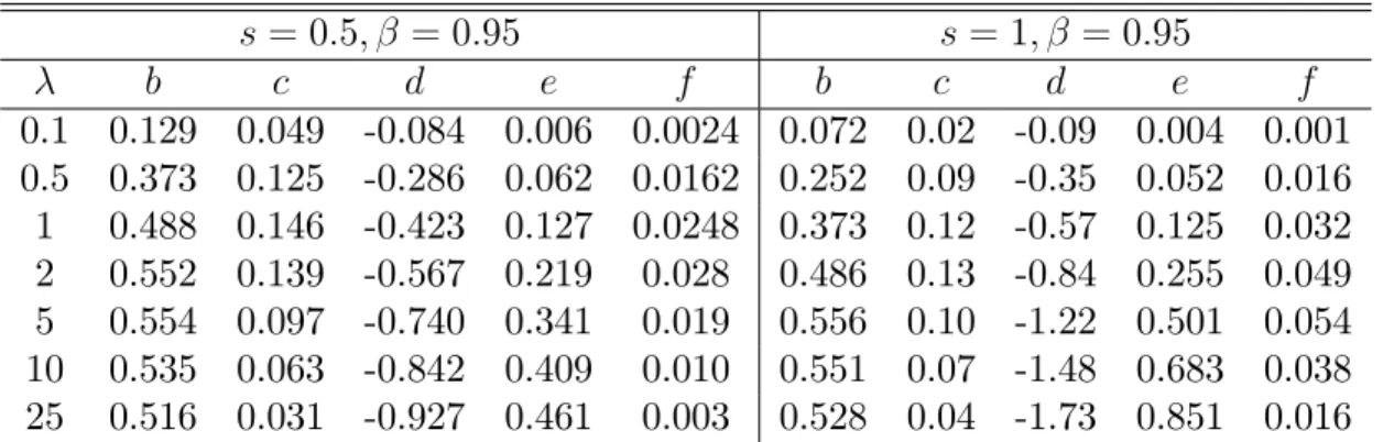
Table A1). Solution for the parameters b; c; d; eand f given values for s; and
s= 0:5; = 0:95 s= 1; = 0:95 b c d e f b c d e f 0.1 0.129 0.049 -0.084 0.006 0.0024 0.072 0.02 -0.09 0.004 0.001 0.5 0.373 0.125 -0.286 0.062 0.0162 0.252 0.09 -0.35 0.052 0.016 1 0.488 0.146 -0.423 0.127 0.0248 0.373 0.12 -0.57 0.125 0.032 2 0.552 0.139 -0.567 0.219 0.028 0.486 0.13 -0.84 0.255 0.049 5 0.554 0.097 -0.740 0.341 0.019 0.556 0.10 -1.22 0.501 0.054 10 0.535 0.063 -0.842 0.409 0.010 0.551 0.07 -1.48 0.683 0.038 25 0.516 0.031 -0.927 0.461 0.003 0.528 0.04 -1.73 0.851 0.016
s= 10; = 0:95 s= 100; = 0:95 b c d e f b c d e f 0.1 0.008 0.003 -0.09 0.0005 0.0002 0.0008 0.0003 -0.09 0.00005 0.00002 0.5 0.038 0.015 -0.47 0.0118 0.0046 0.0041 0.0016 -0.49 0.0013 0.0005 1 0.072 0.027 -0.90 0.0416 0.0159 0.0081 0.0032 -0.98 0.0053 0.0021 2 0.12 0.045 -1.68 0.134 0.0487 0.016 0.0063 -1.95 0.0206 0.0082 5 0.24 0.028 -3.53 0.526 0.165 0.0383 0.0118 -4.75 0.118 0.0465 10 0.33 -0.19 -5.72 1.254 0.325 0.071 -0.014 -9.09 0.416 0.159 25 0.30 -1.45 -8.28 3.100 0.536 0.104 -0.816 -20.3 1.913 0.676
Proof of Proposition 4. First of all, we impose symmetry in the system A3).
Then, we consider the case in which !0:Evaluating the termCat = 0we clearly
obtain that C( =0) = 0, and using this fact into the de…nitions of R and M, we have
that R( =0) = 0; M( =0)= 0: Thus, irrespective of the value ofF; using R( =0) = 0;
M( =0) = 0 into system A3) we have: b = c = d = e = f = 0: Furthermore,
as in Lapham and Ware (1994), the Jacobian matrix associated with that system
is an identity matrix, and thus, non singular. This implies, that at close to zero,
the solution for the unknown parameters is a continuous function of : Substituting
b = d = e = 0 into 10) in the paper, we see that the Markov perfect equilibrium
becomes equal to 21s;that is the static Nash equilibrium given by 11). Now consider
the case in which ! 1:Taking the limit for ! 1of the coe¢ cientsA; B andC,
we obtain lim
!1A = 0; lim!1B = 0 and lim!1C = 1: Applying the well known rules for
limits, we have that lim
!1F = 0; lim!1R = 0 and lim!1M = 1: Thus, taking the limit
for ! 1 of the implicit functions in the system A3) gives the following results for
the unknown parameters: b = 1=2; c = 0; d = 2s ; e = s and f = 0: Again,
substituting this fact into the Markov perfect equilibrium given by 10) we can see that it coincides with the static Nash equilibrium 11). Obviously, we can obtain the
same limit result for the Markov perfect equilibrium, taking the limit for ! 1 of
A4) and applying the Hospital’s rule.
References
[1] Akerlof, G. and J. Yellen (1985), “Can Small Deviations from Rationality Make
Signi…cant Di¤erences to Economic Equilibria?”, American Economic Review
75, pp. 708-721.
[2] Amir, R. (2001), “Stochastic Games in Economics and Related Fields: an
[3] Basar, T. and G.J. Olsder (1995), Dynamic Noncooperative Game Theory, Aca-denic Press: New York.
[4] Cellini, R. and L. Lambertini (2001.a), “Dynamic Oligopoly with Sticky Prices: Closed-Loop, Feedback and Open-Loop Solutions”, Working Paper, Diparti-mento di Scienze Economiche, Universita’degli Studi di Bologna.
[5] Cellini, R. and L. Lambertini (2001.b), “Di¤erential oligopoly Games where the Closed-Loop Memoryless and the Open-Loop Equilibria Coincide”, Working Pa-per, Dipartimento di Scienze Economiche, Universita’degli Studi di Bologna. [6] Cheney W. and D. Kincaid (1999), Numerical Mathematics and Computing,
Brooks/Cole Publishing, Paci…c Grove, CA.
[7] Doganouglu, T. (1999), “Dynamic Price Competition with Persistent Consumer Tastes”, University of Bonn, mimeo.
[8] Driskill R.A. and S. McCa¤erty (1989), “Dynamic Duopoly with Adjustment
Costs: A Di¤erential Game Approach”, Journal of Economic Theory, vol. 49,
pp. 324-338.
[9] Fershtman, C. and M. Kamien (1987), “Dynamic Duopolistic Competition with
Sticky Prices”, Econometrica, vol. 55, no. 5, pp. 1151-1164.
[10] Fudenberg, D. and J. Tirole (1984), “The Fat-Cat E¤ect, the Puppy-Dog ploy,
and the Lean and Hungry Look”,American Economic Review, Papers and
Pro-ceedings 74, pp. 361-389.
[11] Fudenberg, D. and J. Tirole (1991), Game Theory, The MIT Press: Cambridge, MA.
[12] Jensen, H. and B. Lokwood (1998), “A Note on Discontinuous Value Functions
and Strategies in A¢ ne-Quadratic Di¤erential Games”, Economic Letters 61,
pp. 301-306.
[13] Judd, K.L. (1989), “Cournot vs. Bertrand: A Dynamic Resolution”, University of Stanford, mimeo.
[14] Jun, B. and X. Vives (2001), “Incentives in Dynamic Duopoly”, CEPR
Discus-sion Paper, n. 2899 .
[15] Karp, L. and J. Perlo¤ (1993), “Open-loop and Feedback Models of Dynamic
Oligopoly”, International Journal of Industrial Organization, vol. 11, pp.
[16] Kreps, D. and J. Scheinkman (1983), “Quantity Precommitment and Bertrand
Competition Yield Cournot Outcomes”, Bell Journal of Economics, vol.14,
pp.326-337.
[17] Lapham, B. and R. Ware (1994), “Markov Puppy Dogs and Related Animals”, International Journal of Industrial Organization, vol. 12, pp. 569-593.
[18] Leonard D. and N. Van Long (1998), Optimal Control Theory and Static Opti-mization in Economics, Cambridge University Press: Cambridge, UK.
[19] Lockwood, B. (1996), “Uniqueness of Markov Perfect Equilibrium in In…nite
Time A¢ ne-Quadratic Di¤erential Games”, Journal of Economics Dynamics
and Control, vol.20, pp. 751-765.
[20] Mankiw, G. (1985), “Small Menu Costs and Large Business Cycles:
Macroeco-nomic Model of Monopoly”,Quarterly Journal of Economics 100, pp. 529-539.
[21] Maskin, E. and J. Tirole (1987), “A Theory of Dynamic Oligopoly III”,European
Economic Review 31, pp. 947-968.
[22] Maskin, E. and J. Tirole (1988), “A Theory of Dynamic Oligopoly, II: Price
Competition, Kinked Demand Curves, and Edgeworth Cycles”, Econometrica,
vol.56, no. 3, pp. 571-599.
[23] Maskin, E. and J. Tirole (2001), “Markov Perfect Equilibrium: I. Observable
Actions”, Journal of Economic Theory, vol.100, pp. 191-219.
[24] Papavassilopoulos G.P., J.V. Medanic, and J.B. Cruz (1979), “On the Exis-tence of Nash Strategies and Solutions to Coupled Riccati Equations in
Linear-Quadratic Games”, Journal of Optimization Theory and Applications, vol.28,
no. 1, pp.49-76.
[25] Piga, C. (2000), “Competition in a Duopoly with Sticky Prices and Advertising”, International Journal of Industrial Organization 18, pp. 595-614.
[26] Reinganum, J. and N. Stokey (1985), “Olygopoly Extraction of a Common Prop-erty Natural Resource: The Importance of the Period of Commitment in
Dy-namic Games”, International Economic Review, vol. 26, pp. 161-173.
[27] Reynolds, S.S. (1991), “Dynamic Oligopoly with capacity Adjustment Costs”, Journal of Economic Dynamics and Control, vol. 15, no. 3, pp. 491-514.
[28] Rotemberg, J.J. (1982), “Sticky Prices in the United States”,Journal of Political
[29] Slade, M.E. (1999), “Sticky Prices in a Dynamic Oligopoly: An Investigation
of (s; S ) Thresholds”, International Journal of Industrial Organization, vol. 17,
pp. 477-511.
[30] Tirole, J. (1988), The Theory of Industrial Organization, MIT Press: Cambridge, MA.
[31] Zeeuw,A. and J. Van der Ploeg (1991), “Di¤erence Games and Policy Evaluation:
NOTE DI LAVORO DELLA FONDAZIONE ENI ENRICO MATTEI Fondazione Eni Enrico Mattei Working Paper Series
Our working papers are available on the Internet at the following addresses:
http://www.feem.it/Feem/Pub/Publications/WPapers/default.html http://papers.ssrn.com
SUST 1.2002 K. TANO, M.D. FAMINOW, M. KAMUANGA and B. SWALLOW: Using Conjoint Analysis to Estimate Farmers’ Preferences for Cattle Traits in West Africa
ETA 2.2002 Efrem CASTELNUOVO and Paolo SURICO: What Does Monetary Policy Reveal about Central Bank’s Preferences?
WAT 3.2002 Duncan KNOWLER and Edward BARBIER: The Economics of a “Mixed Blessing” Effect: A Case Study of the Black Sea
CLIM 4.2002 Andreas LöSCHEL: Technological Change in Economic Models of Environmental Policy: A Survey VOL 5.2002 Carlo CARRARO and Carmen MARCHIORI: Stable Coalitions
CLIM 6.2002 Marzio GALEOTTI, Alessandro LANZA and Matteo MANERA: Rockets and Feathers Revisited: An International Comparison on European Gasoline Markets
ETA 7.2002 Effrosyni DIAMANTOUDI and Eftichios S. SARTZETAKIS: Stable International Environmental Agreements: An Analytical Approach
KNOW 8.2002 Alain DESDOIGTS: Neoclassical Convergence Versus Technological Catch-up: A Contribution for Reaching a Consensus
NRM 9.2002 Giuseppe DI VITA: Renewable Resources and Waste Recycling
KNOW 10.2002 Giorgio BRUNELLO: Is Training More Frequent when Wage Compression is Higher? Evidence from 11 European Countries
ETA 11.2002 Mordecai KURZ, Hehui JIN and Maurizio MOTOLESE: Endogenous Fluctuations and the Role of Monetary Policy
KNOW 12.2002 Reyer GERLAGH and Marjan W. HOFKES: Escaping Lock-in: The Scope for a Transition towards Sustainable Growth?
NRM 13.2002 Michele MORETTO and Paolo ROSATO: The Use of Common Property Resources: A Dynamic Model CLIM 14.2002 Philippe QUIRION: Macroeconomic Effects of an Energy Saving Policy in the Public Sector
CLIM 15.2002 Roberto ROSON: Dynamic and Distributional Effects of Environmental Revenue Recycling Schemes: Simulations with a General Equilibrium Model of the Italian Economy
CLIM 16.2002 Francesco RICCI (l): Environmental Policy Growth when Inputs are Differentiated in Pollution Intensity ETA 17.2002 Alberto PETRUCCI: Devaluation (Levels versus Rates) and Balance of Payments in a Cash-in-Advance
Economy Coalition
Theory Network
18.2002 László Á. KÓCZY (liv): The Core in the Presence of Externalities Coalition
Theory Network
19.2002 Steven J. BRAMS, Michael A. JONES and D. Marc KILGOUR (liv): Single-Peakedness and Disconnected Coalitions
Coalition Theory Network
20.2002 Guillaume HAERINGER (liv): On the Stability of Cooperation Structures
NRM 21.2002 Fausto CAVALLARO and Luigi CIRAOLO: Economic and Environmental Sustainability: A Dynamic Approach in Insular Systems
CLIM 22.2002 Barbara BUCHNER, Carlo CARRARO, Igor CERSOSIMO and Carmen MARCHIORI: Back to Kyoto? US Participation and the Linkage between R&D and Climate Cooperation
CLIM 23.2002 Andreas LÖSCHEL and ZhongXIANG ZHANG: The Economic and Environmental Implications of the US Repudiation of the Kyoto Protocol and the Subsequent Deals in Bonn and Marrakech
ETA 24.2002 Marzio GALEOTTI, Louis J. MACCINI and Fabio SCHIANTARELLI: Inventories, Employment and Hours CLIM 25.2002 Hannes EGLI: Are Cross-Country Studies of the Environmental Kuznets Curve Misleading? New Evidence from
Time Series Data for Germany
ETA 26.2002 Adam B. JAFFE, Richard G. NEWELL and Robert N. STAVINS: Environmental Policy and Technological Change
SUST 27.2002 Joseph C. COOPER and Giovanni SIGNORELLO: Farmer Premiums for the Voluntary Adoption of Conservation Plans
NRM 31.2002 Carlo GIUPPONI and Paolo ROSATO: Multi-Criteria Analysis and Decision-Support for Water Management at the Catchment Scale: An Application to Diffuse Pollution Control in the Venice Lagoon
NRM 32.2002 Robert N. STAVINS: National Environmental Policy During the Clinton Years
KNOW 33.2002 A. SOUBEYRAN and H. STAHN : Do Investments in Specialized Knowledge Lead to Composite Good Industries?
KNOW 34.2002 G. BRUNELLO, M.L. PARISI and Daniela SONEDDA: Labor Taxes, Wage Setting and the Relative Wage Effect
CLIM 35.2002 C. BOEMARE and P. QUIRION (lv): Implementing Greenhouse Gas Trading in Europe: Lessons from Economic Theory and International Experiences
CLIM 36.2002 T.TIETENBERG (lv): The Tradable Permits Approach to Protecting the Commons: What Have We Learned? CLIM 37.2002 K. REHDANZ and R.J.S. TOL (lv): On National and International Trade in Greenhouse Gas Emission Permits CLIM 38.2002 C. FISCHER (lv): Multinational Taxation and International Emissions Trading
SUST 39.2002 G. SIGNORELLO and G. PAPPALARDO: Farm Animal Biodiversity Conservation Activities in Europe under the Framework of Agenda 2000
NRM 40.2002 S .M. CAVANAGH, W. M. HANEMANN and R. N. STAVINS: Muffled Price Signals: Household Water Demand under Increasing-Block Prices
NRM 41.2002 A. J. PLANTINGA, R. N. LUBOWSKI and R. N. STAVINS: The Effects of Potential Land Development on Agricultural Land Prices
CLIM 42.2002 C. OHL (lvi): Inducing Environmental Co-operation by the Design of Emission Permits
CLIM 43.2002 J. EYCKMANS, D. VAN REGEMORTER and V. VAN STEENBERGHE (lvi): Is Kyoto Fatally Flawed? An Analysis with MacGEM
CLIM 44.2002 A. ANTOCI and S. BORGHESI (lvi): Working Too Much in a Polluted World: A North-South Evolutionary Model
ETA 45.2002 P. G. FREDRIKSSON, Johan A. LIST and Daniel MILLIMET (lvi): Chasing the Smokestack: Strategic Policymaking with Multiple Instruments
ETA 46.2002 Z. YU (lvi): A Theory of Strategic Vertical DFI and the Missing Pollution-Haven Effect SUST 47.2002 Y. H. FARZIN: Can an Exhaustible Resource Economy Be Sustainable?
SUST 48.2002 Y. H. FARZIN: Sustainability and Hamiltonian Value
KNOW 49.2002 C. PIGA and M. VIVARELLI: Cooperation in R&D and Sample Selection Coalition
Theory Network
50.2002 M. SERTEL and A. SLINKO (liv): Ranking Committees, Words or Multisets Coalition
Theory Network
51.2002 Sergio CURRARINI (liv): Stable Organizations with Externalities ETA 52.2002 Robert N. STAVINS: Experience with Market-Based Policy Instruments
ETA 53.2002 C.C. JAEGER, M. LEIMBACH, C. CARRARO, K. HASSELMANN, J.C. HOURCADE, A. KEELER and R. KLEIN (liii): Integrated Assessment Modeling: Modules for Cooperation
CLIM 54.2002 Scott BARRETT (liii): Towards a Better Climate Treaty
ETA 55.2002 Richard G. NEWELL and Robert N. STAVINS: Cost Heterogeneity and the Potential Savings from Market-Based Policies
SUST 56.2002 Paolo ROSATO and Edi DEFRANCESCO: Individual Travel Cost Method and Flow Fixed Costs
SUST 57.2002 Vladimir KOTOV and Elena NIKITINA (lvii): Reorganisation of Environmental Policy in Russia: The Decade of Success and Failures in Implementation of Perspective Quests
SUST 58.2002 Vladimir KOTOV (lvii): Policy in Transition: New Framework for Russia’s Climate Policy
SUST 59.2002 Fanny MISSFELDT and Arturo VILLAVICENCO (lvii): How Can Economies in Transition Pursue Emissions Trading or Joint Implementation?
VOL 60.2002 Giovanni DI BARTOLOMEO, Jacob ENGWERDA, Joseph PLASMANS and Bas VAN AARLE: Staying Together or Breaking Apart: Policy-Makers’ Endogenous Coalitions Formation in the European Economic and Monetary Union
ETA 61.2002 Robert N. STAVINS, Alexander F.WAGNER and Gernot WAGNER: Interpreting Sustainability in Economic Terms: Dynamic Efficiency Plus Intergenerational Equity
PRIV 62.2002 Carlo CAPUANO: Demand Growth, Entry and Collusion Sustainability
PRIV 63.2002 Federico MUNARI and Raffaele ORIANI: Privatization and R&D Performance: An Empirical Analysis Based on Tobin’s Q
PRIV 64.2002 Federico MUNARI and Maurizio SOBRERO: The Effects of Privatization on R&D Investments and Patent Productivity
SUST 65.2002 Orley ASHENFELTER and Michael GREENSTONE: Using Mandated Speed Limits to Measure the Value of a Statistical Life
ETA 66.2002 Paolo SURICO: US Monetary Policy Rules: the Case for Asymmetric Preferences
PRIV 67.2002 Rinaldo BRAU and Massimo FLORIO: Privatisations as Price Reforms: Evaluating Consumers’ Welfare Changes in the U.K.
CLIM 68.2002 Barbara K. BUCHNER and Roberto ROSON: Conflicting Perspectives in Trade and Environmental Negotiations CLIM 69.2002 Philippe QUIRION: Complying with the Kyoto Protocol under Uncertainty: Taxes or Tradable Permits? SUST 70.2002 Anna ALBERINI, Patrizia RIGANTI and Alberto LONGO: Can People Value the Aesthetic and Use Services of