Essays on Environmental and Natural Resource Economics
by
Evan Matthew Herrnstadt
A dissertation submitted in partial fulfillment of the requirements for the degree of
Doctor of Philosophy (Economics)
in the University of Michigan 2015
Doctoral Committee:
Associate Professor Ryan Mayer Kellogg, Chair Associate Professor Jeremy Fox
Assistant Professor Catherine Hausman
©Evan Matthew Herrnstadt
ACKNOWLEDGEMENTS
Thanks are owed to my committee members Ryan Kellogg, Jeremy Fox, Catherine Hausman, and Erich Muehlegger (with whom I co-authored the sec-ond chapter of this dissertation) for consistent support and feedback; to Dan Ackerberg, Varanya Chaubey, Aaron Flaaen, Joe Golden, Max Kapustin, Jason Kerwin, Justin Ladner, Eric Lewis, Johannes Norling, Karen Stockley, Richard Sweeney, Ophira Vishkin, James Wang, and seminar participants at the Uni-versity of Michigan, Resources for the Future, the UniUni-versity of Delaware, and the University of Massachusetts-Amherst for valuable comments; to Mark Anderson, Donovan Asselin, and Doug Heym at the Michigan DNR; and to Phillip Minerick for his insights into the bidding and logging process. Much of the analysis in the first and third chapters was performed on the Univer-sity of Michigan Flux High Performance Computing Cluster. I gratefully ac-knowledge funding from the Joseph L. Fisher Dissertation Fellowship from Resources for the Future and from the Michigan Institute for Teaching and Research in Economics.
TABLE OF CONTENTS
DEDICATION . . . ii
ACKNOWLEDGEMENTS . . . iii
LIST OF FIGURES . . . vi
LIST OF TABLES . . . viii
LIST OF APPENDICES . . . ix
ABSTRACT . . . x
CHAPTER 1. Conservation Versus Competition? Environmental Objectives in Government Con-tracting . . . 1
1.1 Abstract . . . 1
1.2 Introduction . . . 2
1.3 Policy and Empirical Setting . . . 6
1.3.1 Environmental Objectives and Fostering Competition . . . 6
1.3.2 Timber Contracts and Seasonal Restrictions . . . 7
1.4 Features of the DNR Contract Data . . . 10
1.4.1 Contract Characteristics and Auction Outcomes . . . 10
1.4.2 Seasonal Restrictions . . . 12
1.5 The Effect of Restrictions on Equilibrium Bidding . . . 12
1.5.1 Main Specification . . . 13
1.5.2 Robustness: Identification from Multiple Restriction Types . . . 15
1.5.3 Importance of the Participation Margin . . . 16
1.6 A Structural Model of DNR Timber Auctions . . . 17
1.6.1 Main Assumptions . . . 17
1.6.2 Potential Effects of Seasonal Restrictions on Bids . . . 19
1.6.3 Parameterizing the Model . . . 22
1.6.4 Empirical Implementation of the Model . . . 24
1.7 Results of the Structural Estimation . . . 27
1.7.1 Parameter Estimates and Model Fit . . . 27
1.7.2 Effect of Restrictions on Agent Payoffs . . . 28
1.7.3 Optimal Reserve Prices. . . 30
1.7.5 Policy Implications . . . 33
1.8 Conclusion . . . 34
1.9 Figures . . . 37
1.10 Tables . . . 59
2. Weather, Salience of Climate Change, and Congressional Voting . . . 68
2.1 Abstract . . . 68
2.2 Introduction . . . 68
2.3 Methodology . . . 72
2.3.1 Data. . . 72
2.3.2 Empirical Approach . . . 74
2.4 Weather and Search Intensity Results . . . 77
2.5 Weather, Search Intensity and Voting Behavior. . . 80
2.6 Conclusion . . . 90
2.7 Figures . . . 91
2.8 Tables . . . 94
3. Seller Commitment and the Empirical Analysis of First-Price Auctions . . . 99
3.1 Abstract . . . 99
3.2 Introduction . . . 100
3.3 Model Setup and Equilibrium. . . 104
3.3.1 Model . . . 104
3.3.2 Proof of Cutoff Equilibrium . . . 105
3.4 Identification . . . 108
3.4.1 Nonparametric Identification . . . 109
3.4.2 The Importance of EstimatingFω . . . 111
3.4.3 A Semiparametric Approach . . . 113
3.5 Monte Carlo Simulation. . . 113
3.6 Application: Auctions for DNR Timber Contracts . . . 115
3.6.1 DNR Timber Auctions and the Reserve Price Policy . . . 115
3.6.2 Is the Model Appropriate? . . . 117
3.7 Incorporating Unobserved Auction Heterogeneity . . . 119
3.8 Conclusion and Future Work . . . 121
3.9 Figures . . . 123
3.10 Tables . . . 129
Appendices . . . 133
LIST OF FIGURES
FIGURE
1.1 Sample seasonal restriction . . . 37
1.2 Sales per quarter, by peninsula . . . 37
1.3 Michigan DNR Forest Management Units . . . 38
1.4 Distribution of months of restrictions . . . 39
1.5 Log winning bid . . . 40
1.6 Number of bidders . . . 41
1.7 Participation rate . . . 42
1.8 Log winning bid, controlling for potential bidders . . . 43
1.9 Log winning bid, controlling for restriction categories . . . 44
1.10 Number of bidders, controlling for restriction categories . . . 45
1.11 Log winning bid, controlling for number of bidders . . . 46
1.12 Moments of value distributions at mean X values . . . 47
1.13 Distribution of auction-specific valuation parameters . . . 48
1.14 Comparing winning bids in all auctions receiving bids . . . 49
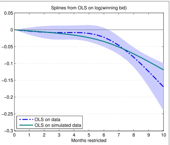
1.15 Splines from log winning bid regressions . . . 50
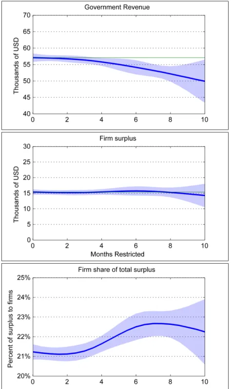
1.16 Mean auction outcomes, by level of seasonal restrictions . . . 51
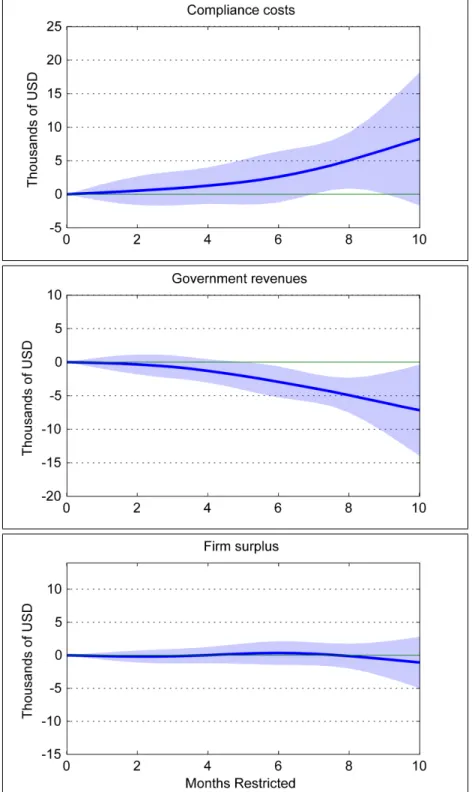
1.17 Changes in mean auction outcomes, by level of seasonal restrictions . . . 52
1.18 Relative changes in surplus . . . 53
1.19 Relative impact of restrictions under different reserve price regimes,v0 = 0 . . . 54
1.20 Relative impact of restrictions under different reserve price regimes,v0 =Robs . . . . 55
1.21 Revenues across reserve price regimes,v0 = 0 . . . 56
1.22 Revenues across reserve price regimes,v0 =Robs . . . 57
1.23 Decomposition of equilibrium bid effect: Mechanisms . . . 58
2.1 Average temperature deviations, 1974-2011 . . . 91
2.2 Plot of residuals: Colorado, Oct. 2006-Apr. 2007 . . . 92
2.3 All climate-related searches compared to skeptical searches . . . 92
2.4 Environmental vote share for LCV-tracked votes . . . 93
2.5 Estimated effect of search on voting by member’s overall LCV score . . . 93
3.1 Performance of Naive Estimator ofF1 . . . 123
3.2 Monte Carlo Estimates ofFω . . . 124
3.3 Monte Carlo Estimates ofF2 (Untruncated) . . . 125
3.4 Monte Carlo Estimates ofF2 (Truncated at true or mean estimatedv∗) . . . 126
3.6 Time gap between first and second round . . . 128
A.1 Average months of restrictions, by season . . . 138
A.2 Restrictions in various seasons, by total months restricted. . . 139
A.3 Marginal effect of an additional month in a given season . . . 140
A.4 Number of sales appraised by each forester . . . 141
A.5 Distribution of instrumental variable . . . 141
A.6 Distribution of instrumental variable, demeaned within MU . . . 142
A.7 Distribution of instrumental variable, standardized within MU . . . 142
B.1 Missing observations, 2004-2007 . . . 148
B.2 Missing observations, 2008-2011 . . . 149
LIST OF TABLES
TABLE
1.1 Major restriction categories . . . 59
1.2 Summary statistics . . . 60
1.3 DNR Cost Factor Criteria . . . 60
1.4 Linear regressions, log winning bid . . . 61
1.5 Linear regressions, number of bidders . . . 62
1.6 Pairwise combinations of restrictions . . . 63
1.7 Linear regressions controlling for restriction categories . . . 64
1.8 Estimated structural parameters . . . 65
1.9 Model fit: sample moments . . . 65
1.10 Model fit: Winning bid OLS . . . 66
1.11 Mean outcomes considering optimal reserve prices,v0 = 0 . . . 66
1.12 Mean outcomes considering optimal reserve prices,v0 =Robs . . . 67
1.13 Decomposition schematic: Mechanisms . . . 67
2.1 Descriptive Statistics, Full Sample . . . 94
2.2 Weather correlations . . . 94
2.3 Effect of weather deviations on search intensity . . . 95
2.4 Environmental Votes, Local Weather and Search Intensity . . . 96
2.5 ACU Votes, Local Weather and Search Intensity . . . 97
2.6 Environmental Votes and Search Intensity, by Representative Characteristics . . . 97
2.7 Environmental Votes and Search Intensity, by Vote Characteristics . . . 98
3.1 Parameterization of Monte Carlo . . . 129
3.2 Monte Carlo Results . . . 129
3.3 DNR Regressions. . . 130
3.4 Round-by-Round Contracting Outcomes . . . 131
3.5 Exploring unobserved heterogeneity assumptions . . . 132
A.1 Linear regressions, effects of different seasons . . . 143
A.2 TSLS regressions . . . 144
B.1 Robustness to Missing Data . . . 151
B.2 Robustness to Balanced Panel 2007-2011 . . . 152
B.3 Regressions by Month . . . 153
B.4 Sensitivity to the Inclusion of Various Fixed Effects. . . 154
LIST OF APPENDICES
APPENDIX
A. Appendices for Chapter 1 . . . 133
B. Appendices for Chapter 2 . . . 145
ABSTRACT
Essays on Environmental and Natural Resource Economics by
Evan Matthew Herrnstadt
Chair: Ryan M. Kellogg
This dissertation addresses issues in the economics of the environment and natural resources. The first chapter pertains to the inclusion of environmental objectives into contracts between the government and private firms. In particular, it considers the possibility that conservation restric-tions may undermine the goal of fostering competition among private logging firms in timber auctions. Empirically, the policy is costly but is found to be borne primarily by the state without substantial competitive distortions. Importantly, that state can reduce the impact of the policy on revenues by setting reserve prices optimally.
The second chapter is joint work with Professor Erich Muehlegger. We use data on Google search activity related to climate change and shocks to local weather to demonstrate that unusual weather increases the salience of climate change as an issue. Further, we find that recent weather shocks have a significant effect on Congressional votes pertaining to environmental regulation.
The third chapter makes a methodological contribution to the analysis of auction data. Many auctions have a reserve price, below which the seller simply keeps the object of interest. However, it is typically taken for granted that the object will not be re-auctioned later. Empirical researchers
should account for the fact that bidders may respond to this possibility. I present a simple model of repeat auctions, discuss what information can be identified from bidding data, and provide a Monte Carlo simulation of an estimator that addresses this issue. Finally, I examine data on repeat auctions of logging contracts to see whether bidding behavior is consistent with the model. These data could provide a context in which to estimate the model and analyze counterfactual auction policies.
CHAPTER 1.
Conservation Versus Competition? Environmental
Objectives in Government Contracting
1.1
Abstract
Government contracts with private firms increasingly incorporate environmental objectives or pref-erences for sustainable products and producers. At the same time, the government often solicits competitive bids to reduce the rents captured by the firms due to private information. In this paper, I show how environmental objectives can influence equilibrium contract bids through changes to firm costs, strategic bidding behavior, and bidder participation decisions. Using data from Michi-gan state logging contracts, I find that conservation objectives reduce bidder participation in the contract auctions by up to 35 percent and depress winning bids by up to 17 percent. To disentangle compliance costs from logger margins, I estimate a structural model of the auctions. Simulations based on the estimates imply that the policy imposes economically and statistically significant compliance costs. Loggers are able to completely pass these costs on to the government because compliance costs do not substantially affect the dispersion of private values. However, the use of optimal reserve prices partially mitigates the revenue disparity between more- and less-restricted contracts. Finally, loggers capture a larger share of total auction surplus for restricted contracts, indicating that the policy undermines the state’s ability to harness competition to capture surplus.
1.2
Introduction
Increasingly, governments are leveraging the scale and scope of their contracts with private firms to reduce the environmental impact of large projects and purchases. At the same time, contracts issued by the government are often awarded to firms through competitive bidding to increase rev-enues (in the case of a sale) or reduce costs (in the case of a purchase). While the pursuit of environmental objectives will likely impose additional costs on the firms, the economic incidence of these costs will be determined by the intensity of competitive pressure among bidders. Indeed, previous work has recognized that the pursuit of social objectives in government auctions, such as small-business preferences or bids based on estimated contract completion time, can distort com-petition and affect government revenues, bidder surplus, and efficiency.1 Unlike these policies that
typically modify the rules of the allocation mechanism, environmental objectives often affect the value of the contract itself. However, such objectives can still undermine or bolster competition.
In this paper, I estimate the effect of environmental objectives on competitive pressure in auc-tions for natural resource extraction contracts. In particular, I analyze competition for timber con-tracts auctioned by the State of Michigan Department of Natural Resources (DNR) in the presence of varying seasonal operating restrictions. The restrictions are implemented to mitigate the im-pacts of logging in the state forests on the surrounding ecology and recreational use. I identify a large, negative effect on equilibrium bids and logger participation by exploiting the structure of the seasonal restrictions and a rich set of controls.2 To quantify the relative importance of the cost of complying with the restrictions versus that of weakened competition, I estimate a structural model of the DNR-administered first-price timber auctions. The bidders’ value distribution is parameter-ized so that it depends flexibly on the seasonal restrictions. I find that most of the effect on bids is driven by lower valuations, and that the loggers are able to pass nearly the full cost of compliance
1Examples of this literature include Marion (2007); Krasnokutskaya and Seim (2011); Athey, Coey, and Levin (2013); and Bajari and Lewis (2011).
2Throughout the paper, I refer to all potential bidders as “loggers” for narrative simplicity. In several other papers that model timber auctions (Athey, Levin, and Seira, 2011; Roberts and Sweeting, 2013), the authors distinguish between loggers and mills. Conversations with DNR employees suggest that there are few large-scale mills operating in this market.
through to the DNR.
The reduced-form analysis demonstrates that environmental objectives have a negative effect on bids and auction participation and suggests that differential competition could play an important role. Specifically, I estimate that the winning bid is 17 percent lower for the most-restricted timber contracts and that these contracts receive 35 percent fewer bids above the reserve price. However, these effects are highly nonlinear; if the contract is restricted for fewer than 5 months, the bids are not significantly different from bids for the unrestricted contracts. Moreover, these estimates are robust to controlling for the underlying reasons for the restrictions, which mitigates concerns about omitted variable bias. Finally, controlling for the number of participating bidders accounts for half of the effect of restrictions on the winning bid, which suggests that the participation margin matters, but is not driving the entire effect of restrictions.
Although the reduced-form analysis of equilibrium bids estimates the effect of restrictions on government revenue, it cannot generally reveal how costly the restrictions are or who bears the economic burden of these costs. If the restrictions cause logger valuations for a contract to become more dispersed, loggers will be more insulated from competition and the winning bidder’s equilib-rium surplus will increase. In contrast, if the restrictions compress the distribution of valuations, loggers will expect more intense competition and the winning bidder’s equilibrium surplus will decrease.
To disentangle these effects, I specify a model of the DNR’s first-price auctions and analyze the three channels through which restrictions result in lower bids. First, the bidders’ values could be lower, directly resulting in reduced bids. Second, the bidders would further depress their bids if they face less competition locally because of increased dispersion in private values. Third, firms may change their decision to participate in the auction altogether.
I structurally estimate the auction model and find that compliance with stringent environmental objectives is costly. These costs are almost completely borne by the government. Compliance costs are very close to zero for contracts that are restricted for less than 4 months. However, restrictions covering 10 months of the year create compliance costs amounting to 15 percent of the government
revenue or 54 percent of the firm surplus from an unrestricted sale. Even when the sale is restricted for only 6 months, the compliance costs amount to 5 percent of government revenue or 17 percent of firm surplus. I find that loggers are able to depress their bids enough to fully pass through the compliance costs to the state. The change in average firm surplus is precisely estimated and very close to zero for most levels of restrictions. I also find that setting optimal reserve prices can close some of the revenue gap between more- and less-restricted sales.
The full passthrough finding is driven by two factors. First, I assume that the DNR is perfectly inelastic to expected bids in supplying timber contracts. This assumption is supported by the timing of and institutional criteria driving the timber harvest process. Second, my estimates suggest that compliance costs do not affect the dispersion of contract values. Thus, firms face a similar “local” distribution of opponents. These mechanisms are related to those discussed by Fabra and Reguant (2014), who estimate full pass-through of carbon permit costs in the wholesale Spanish electricity market.
A different way to evaluate the effect of restrictions on auction competition is to calculate the share of total surplus (government revenue plus firm surplus) captured by loggers. I find that for an average contract, loggers capture a 5.2 to 6.6 percent larger share of surplus for more restricted sales relative to unrestricted sales; the difference is statistically significantly different from zero. This indicates that the restrictions do undermine the competitive performance of the timber auc-tions, even though thelevelof firm surplus falls slightly.
To better understand the relative importance of various mechanisms, I decompose the effect of restrictions on bids. Holding bidding strategies fixed for a logger with a given valuation, I find that lower valuations due to restrictions directly account for 73 to 82 percent of the decrease in bids. Allowing loggers to revise their bidding strategies and participation decisions in response to their opponents’ now-lower valuations accounts for the remaining 18 to 27 percent. This decom-position shows that the change in winning bids reflects a substantial adjustment by loggers to the compliance costs of their competitors.
used in a variety of settings. For example, drilling for oil and gas on government-issued leases is seasonally restricted, both onshore and offshore, for a variety of environmental reasons. Past and existing ozone regulations have often had seasonal components, such as the NOx Budget Program/SIP call and various gasoline content requirements. Finally, seasonal restrictions also arise frequently in the context of regulated fisheries to prevent adverse effects on non-target species. Furthermore, environmental objectives are increasingly embedded in a wide variety of govern-ment contracting settings. While the Competition in Contracting Act of 1984 sets out conditions and exceptions regarding free and open bidding on federal contracts, various statutes allow the federal government to relax the Act’s requirements to pursue goals related to the environment and sustainability. For instance, the Obama Administration has issued a series of executive orders that promote consideration of environmental factors in federal procurement. In addition, the Gen-eral Services Administration is considering incorporating bidders’ greenhouse gas emissions as a criterion in the federal procurement process. Finally, the planning and completion of contracted projects (e.g., highway construction) may be subject to broader environmental regulation, such as the National Environmental Protection Act, the Clean Air Act, and the Clean Water Act.
Governments should be aware that environmental objectives can distort the competitive struc-ture of the contracting process, rendering simple policy predictions and evaluations inaccurate. Strategic firm responses can be an important consideration when evaluating the impacts of various environmental policies (Busse and Keohane, 2007; Brown, Hastings, Mansur, and Villas-Boas, 2008; Ryan, 2012). An ex ante prediction of future bids based on estimated compliance costs assumes exact one-to-one pass-through, which does not have to be the case. Conversely, an ex post regulatory cost calculation from a simple comparison of bids with and without the environ-mental policy ignores the potential impact of changing firm margins. An understanding of the competitiveness of the market is crucial for an accurate evaluation.
I organize the remainder of the paper as follows: In Section 2, I describe the market for logging contracts in Michigan and outline the role of seasonal operating restrictions. In Section 3, I describe the contract data and discuss my measure of seasonal restrictions. In Section 4, I establish
reduced-form effects of the restrictions on equilibrium bid outcomes. In Section 5, I develop and explain the implementation of the structural model. In Section 6, I present the structural parameter estimates, discuss the magnitude of compliance costs and the incidence of the seasonal restrictions, consider an optimal reserve price policy that depends on the restrictions, and decompose the reduced-form effect to shine light on the importance of various mechanisms at play. Section 7 concludes the paper.
1.3
Policy and Empirical Setting
To provide context for the empirical analysis, I describe the widespread inclusion of environmental objectives in government contracting. I also outline my specific context: Michigan DNR logging contract auctions. These contracts include seasonal operating restrictions that protect the ecologi-cal integrity of the forest and promote multiple uses, but may impose costs on loggers by reducing scheduling flexibility.
1.3.1
Environmental Objectives and Fostering Competition
Governments rely heavily on goods and services outsourced from private firms. When they contract with such firms, there is an information asymmetry: the firms have better information about their own productivity levels, costs, or values for the contract. The government often uses a competitive bidding process to extract this information; however, firms will still capture some information rents. One indicator of the competitiveness of this process is the share of total surplus that the firm manages to capture in information rents.
Although government contracting is generally carried out with a priority of fostering compe-tition, environmental responsibility is one competing concern. In the federal context, the Compe-tition in Contracting Act of 1984 states that contracts are to be awarded through “full and open competition”, with potential exceptions for small business set-asides, an urgent and compelling need, a service with a sole supplier, small purchases, or other reasons authorized in statute.
Envi-ronmental preferences and objectives are justified under a number of statutes across a wide variety of contracting settings. While the competitive impact of the small business exception has been well-studied (Marion, 2007; Krasnokutskaya and Seim, 2011; Athey, Coey, and Levin, 2013), en-vironmental objectives have not.3
Such environmental objectives are becoming more pervasive: many federal government agen-cies have established broad “Green Procurement Programs” to comply with a variety of relevant executive orders and congressional acts (Manuel and Halchin, 2013). Some agencies have ex-pressed concerns that these practices will considerably shorten the list of acceptable contractors or products (United States Department of Defense, 2008). An important, and not easily measured, component of evaluating these programs is whether they affect the competitive performance of the bidding process in terms of the division of surplus. I analyze conservation and multiuse require-ments in Michigan state forest logging contracts to illustrate the possible effects of environmental objectives on competition for government contracts.
1.3.2
Timber Contracts and Seasonal Restrictions
The Michigan DNR is mandated with maintaining the ecological integrity and promoting the recre-ational use of the state forests, while supporting the timber and timber products industry by auc-tioning logging contracts.4 These logging contracts often include clauses that disallow operations during certain times of the year during which the forests are ecologically-sensitive or subject to high recreational demand. The restrictions are known prior to the competitive bidding process. Loggers claim that these restrictions can be quite costly to their operations and affect their bids.
The DNR tracks the condition of the Michigan state forest system on an ongoing basis. Foresters survey each forest compartment (roughly 2000 acres) every 10 years. This survey includes
infor-3Aral, Beil, and Wassenhove (2014) theoretically analyze a company that decides whether to audit possible suppli-ers for sustainable practices prior to a private procurement auction. Smith, von Haefen, and Zhu (1999) compare the cost per mile of highway construction in states with a higher or lower likelihood of triggering federal environmental and cultural preservation review requirements.
4This mandate is similar in spirit to the federal Multiple Use-Sustained Yield Act governing the mission of the U.S. Forest Service.
mation about the basic mix, density, and health of the compartment to be used in a statewide timber inventory. Each year, the foresters determine which stands of trees will be contracted for harvest using a combination of inventory and aerial data. According to conversations with DNR officials, the timber is chosen for harvest to pursue forest-management goals. That is, trees are harvested to maintain proper age balance, density, and disease and pest resistance. Once a stand of trees is selected for commercial harvest, the DNR sends a forester out to the stand to obtain more precise measurements of the timber to be harvested. In the process, the forester may determine that there are grounds for seasonal operating restrictions. For instance, if the ground is particularly wet in the summer, operations may not be allowed during that time of year to prevent damage to the forest’s root structure.
Once the survey is completed, the DNR holds an auction for the obligation to harvest the timber. A contract is made public, including any seasonal restrictions. There is usually a 4-6 week bidding period before the bid opening date. During the interim, loggers often conduct a “cruise” of the sale to get a first-hand look at the area in which the harvest will take place. The auctions are sealed-bid first-price auctions with public reserve prices. The sealed-bids, sealed-bidder identities, and number of sealed-bids submitted are considered confidential until the results are made fully public at the bid opening. The highest bidder wins the contract, pays a down payment, and is obligated to harvest the specified timber before a contract deadline. Failure to fulfill the contract terms results in a financial penalty and possible exclusion from future sales.5
Seasonal operating restrictions are added to timber contracts to help protect the ecological integrity and recreational accessibility of the state forests while they are harvested. To this end, the contracts will often specify certain dates during which the loggers cannot operate on the sale. There are a number of reasons that a sale might be restricted in such a way; Table 1.1 provides the frequency with which the main reasons are cited. Many of these restrictions are related to environmental conservation and resource management. For instance, many sales are restricted in the spring/summer due to “bark slip”. From April through July, tree bark tends to loosen from the
trunk. Thus, it is easy to damage trees when cutting and hauling nearby timber. An example of such a contract clause is displayed in Figure1.1. Another example is the presence of an endangered bird, which would require operations to cease during nesting season. There are also restrictions related to the multiuse mandate of the state forest system: areas with popular snowmobile trails are sometimes restricted during winter months, while an area with a large deer population might be restricted during hunting season.
There is some existing empirical evidence that such restrictions influence a logger’s bidding decision for a given contract. Using data from Minnesota state forest auctions, Brown, Kilgore, Coggins, and Blinn (2012) find that sales that allow harvesting activity during the summer or fall garner winning bids that are 7 percent higher. Taking a different approach, Brown, Kilgore, Coggins, Blinn, and Pfender (2010) surveyed loggers and DNR foresters in Michigan, Minnesota, and Wisconsin. Loggers cited seasonal restrictions as the most important factor for determining their bids, aside from the volume and type of timber included in the contract.
Conversations with Michigan loggers and DNR foresters suggest that these restrictions are costly primarily because they impose scheduling constraints. Loggers attempt to keep their equip-ment running year-round for three main reasons. First, many loggers have quotas and contracts with sawmills and pulpmills that they need to meet at some frequency. Second, logging can be quite capital-intensive, and consistent revenues are needed to stay up-to-date on loan payments. Third, loggers simply want to provide consistent employment for their workers. This desire to schedule jobs throughout the year leads to a difficult scheduling problem.6 The scheduling
prob-lem becomes more complicated when the sales are seasonally restricted. Essentially, a restricted sale embodies less option value than one that can be cut at any time of year.
These types of restrictions would be less costly if there was a well-functioning short-term equipment rental market. However, a survey of loggers located in the Eastern half of the Upper Peninsula and the Northern Lower Peninsula suggests that rental activity is limited. In 2009, firms used self-owned equipment for an average of 89 percent of their total operations. An average of
19 percent of operations was performed using subcontracted equipment, but this question was only answered by about half of the respondents and the minimum response was 1 percent. Assuming that the non-responding firms did not subcontract at all, 10 percent of total operations used some subcontracted equipment. Although the share is non-negligible, it is small. Furthermore, the cost of the restrictions is likely related to unexpected shocks. Such short-run rentals would be even more difficult to transact.
1.4
Features of the DNR Contract Data
In this section, I outline the key outcomes and covariates from the contract data. I also construct a measure of seasonal restrictions, which shows that there is considerable variation in the number of months for which a contract is restricted. I will use this variation to estimate a flexible relationship between restriction intensity and bidding behavior, private values, and participation costs.
1.4.1
Contract Characteristics and Auction Outcomes
I obtained the contract text and auction outcomes for all Michigan state commercial timber sales from April 2004 - March 2013. The data include extensive information about the contract and auction outcomes, such as all bids, bidder identities, reserve prices, DNR volume estimates of each product-species combination in the sale, acreage, DNR cost factor estimates, and precise sale location. To scale bids and reserve prices in a way that makes sales more comparable, I re-express bids and reserve prices in dollars per thousand board feet (MBF).7 Reserve prices are set using a formula based on recent prices paid for the same species in the same state forest.
Table1.2presents a summary of the sample auctions. Of the 5207 sample auctions, 457 receive zero bids. Conditional on receiving at least one bid, the mean sale receives a winning bid of $92.2/MBF; in total dollar terms, the DNR earns $66,000 in revenue from the average contract
7For reference, 1 MBF of lumber would be a stack of boards that is 10 feet long, 4 feet wide, and just over 2 feet tall. To convert pulpwood, which is measured in cords, to MBF, I use a conversion rate of 2 cords per MBF (Mackes, 2004). I include controls for the composition of the sale in all specifications.
transaction.8 The mean reserve price is $61.6/MBF, or roughly $43,000. The median number of bidders is 3, and the mean is 3.9, reflecting a long right tail (the maximum number of bidders in a single auction is 19). I measure potential bidders by identifying the set of loggers that are active in similar auctions. Specifically, I define a potential bidder to be any logger who bids for a state forest contract in the same calendar quarter and DNR management unit as the contract of interest.9 This
definition seems reasonable: 87 percent of bidders in a given auction bid in at least one other state timber auction in the same calendar quarter-management unit. There are a mean of 18 potential bidders for the contracts, and the participation rate in a typical auction is approximately 20 percent. The value of a contract will vary based on the type of timber required to be harvested and the attributes of the harvest site itself. The average sale is about 83 percent pulpwood by volume. Pulpwood comes from smaller-diameter trees and parts of trees and is sold to make paper products. Sawlogs, which are used to make lumber and utility poles, account for the other 17 percent. There is considerable variation in the sample, both in terms of the proportion of pulpwood versus sawlogs and the proportion of softwood (such as pine) versus hardwood (such as walnut). The cost factor variable captures attributes such as wetness, slope, and distance to a road. It is generated by the forester appraising the sale on the ground, and is used to help inform the appraisal/reserve price.
I restrict the sample slightly to exclude especially unusual sales. I exclude sales with reserve prices less than $20/MBF or greater than $250/MBF or areas less than 20 acres or greater than 640 acres. These roughly represent the 1st and 99th percentiles of these variables. I also drop all salvage sales, which specifically market fire-, wind-, or pest-damaged timber. Figure1.2presents the number of sample auctions that took place each quarter in the Lower and Upper Peninsulas. Clearly there is some cyclicality in both peninsulas – there are generally more sales held in spring and summer than in winter and fall. Given that the median contract lasts nearly 2.5 years, season of the auction itself should not play a large role in the value of the contract. Still, I include quarter-of-year dummy variables in my primary specification to control for this pattern and find that it does
8All dollar figures are deflated to 2009 USD.
9A management unit is usually a 2 to 3 county area: see Figure1.3for a map. This general approach is similar to existing work that analyzes entry in timber auctions, such as Roberts and Sweeting (2013) and Athey, Coey, and Levin (2013).
not have a large effect on my results.
1.4.2
Seasonal Restrictions
The DNR does not maintain a database variable that indicates when harvesting operations are allowed. However, the information is written into the contract that describes the sale to potential bidders. Thus, I analyzed all relevant contract clauses and constructed such a variable. Specifically, I calculated the number of months that a sale is restricted.10 This variable captures the first-order
driver of lost option value: the number of months during which a sale is inaccessible.11
There is considerable variation in the average number of months for which a sale is restricted. Among sales with any restrictions, the median is 3 months, which reflects that many sales are restricted for a single season. However, there are 536 contracts (10.2 percent of the full sample) that are restricted for 6 or more months. Figure1.4displays the conditional distribution of restrictions. The spike at the 2-3 month bin reflects that the most common restriction (bark slip) generally lasts between 2 and 3 months, from mid-April to mid-July.
1.5
The Effect of Restrictions on Equilibrium Bidding
In this section, I show that seasonal restrictions have a negative effect on equilibrium bidding and participation. First, I estimate the effect of seasonal restrictions on winning bids and the number of bidders participating in an auction, controlling for a rich vector of auction characteristics. Second, I demonstrate robustness of this base specification to omitted variables by exploiting the structure of the seasonal restrictions. Third, I establish suggestive evidence that some of the effect on bids is driven by changes in competition.
10Sales are divided into “payment units”, which may be subject to different restrictions. For each calendar month, I determine the fraction of the month that each payment unit is restricted. Then I calculate the average across payment units, weighting them by appraisal value.
11One concern with this measure is that if a contract takes a few weeks to fulfill, then a short window of availability is essentially a restriction. Less than 1 percent of contracts have any windows between restrictions that last for 15 days or less. Treating these windows as restrictions or omitting such sales from the analysis entirely has no effect on the results. In Appendix A, I also consider seasonality as a possible mechanism.
1.5.1
Main Specification
I estimate a large, negative effect of restrictions on bids and participation. When the restrictions are allowed to enter nonlinearly into the regression, I find that the effects are concentrated among the more-restricted sales.
The main specification is given by:
Outcomea=h(M onthsRestricteda) +βXa+εa
whereOutcomeais the number of bidders or the logarithm of the winning bid per MBF in auction
a,h(·)is a function of the number of months for which a contract is restricted, andXais a vector of
controls. These controls contain standard characteristics used in previous work on timber auctions, such as the Herfindal-Hirschman Index of the value of the species in the sale, the size of the sale in acres, and the mix of sawlogs (lumber) versus pulpwood (a paper input).12 A particularly important and new control variable is a cost index developed by the DNR. This index is meant to capture otherwise difficult-to-capture characteristics, such as the topography of the land, the soil conditions, road and construction requirements, the distance to the nearest road and mill, and an assessment of the timber quality. Importantly, seasonal restrictions are not directly accounted for in these cost factors. Table1.3 further describes the criteria used in developing the cost factors. Note that this variable is defined such that a larger value corresponds to alesscostly sale.
Although seasonal restrictions may be correlated with other determinants of a contract’s value, I address much of the omitted variable problem with a comprehensive set of controls and proxies. For example, if a wet stand of timber is more likely to be restricted to preserve the root structure of the stand, but loggers also find working in wet areas more costly due to higher equipment main-tenance costs, this would introduce negative bias into the treatment effect. Most of these concerns can be eliminated by controlling for observable auction characteristics. The DNR-calculated cost index is a particularly crucial control variable for this reason. In Section1.5.2, I also leverage the
structure of the restrictions. In particular, contracts are frequently restricted for multiple reasons, which allows me to control for the underlying basis for the restrictions.
When I specify h(·) as a linear function of the months of restrictions, I find that restrictions have a significant negative effect on the logarithm of winning bids and the number of bidders (see Tables1.4and1.5, respectively).13 The effect of an additional month of restriction is quite robust
across different sets of controls and location, quarter-of-year, and year fixed effects. I focus on Column 4 as my preferred specification for both the reduced-form and structural estimates. This specification indicates that that the most-restricted contracts attract 8 percent less revenue and 0.8 fewer bidders out of an average of 3.9.
Although the linear functional form implies that the additional effect of each month of restric-tions is the same, estimates from a more flexible specification suggest that the state should be primarily concerned about losing revenues due to the most stringent restrictions. When I specify
h(·)as a restricted cubic spline with knots at 0, 3, 6, and 10 months of restrictions, the effects are strikingly different from the linear effect.14 Figures 1.5 and 1.6 present the cumulative effect of
restrictions as the number of months increases from zero to 10 (the maximum in the sample) on the logarithm of the winning bid and the number of bidders, respectively.15 The first four months of restrictions have zero marginal effect on winning bids, while the average marginal effect over restriction months 5-10 is about 4 percent per month. In contrast, the linear specification implies that each additional month of restrictions is associated with a 0.8 percent decline in the winning bid. For a contract that is restricted for 10 months, the effect is quite large: it receives 1.5 fewer bids (the mean is 3.9) and a winning bid that is 17 percent lower relative to an unrestricted contract. The effect on the number of bidders suggests that the differences in winning bids might be driven by differences in market thickness. Suppose that seasonal restrictions are more prevalent in areas with fewer active loggers. Then we would expect more restricted sales to attract a different number of bidders and level of bids even without a causal effect of restriction on bidding behavior.
13As contracts in the same area around the same time are likely to be subject to similar shocks, I calculate clustered standard errors at the county-by-year level.
14The results are robust to other similar sets of knots.
Figure 1.7 shows that a lower share of potential bidders actually participate in auctions for the more-restricted sales. Furthermore, in Figure1.8 I replicate the regression in Figure 1.5, except that I control for a flexible polynomial of the number of potential bidders. The treatment effect does not change appreciably, indicating that the reduced-form results are not driven by differential market thickness.
1.5.2
Robustness: Identification from Multiple Restriction Types
To this point, the identification assumption has been that, conditional on control variables, the re-strictions only affect values directly through the scheduling constraint and are also uncorrelated with other unobserved determinants of bids. Given that the restrictions do not require specific procedures during the time that the sale is accessible, this seems reasonable. To further address potential omitted variable bias, I exploit the fact that a single contract could be restricted for mul-tiple unrelated reasons. Specifically, I control for the rationales behind the restrictions with a set of dummy variables.16 The new weaker identification assumption is that theinteractionsbetween
restriction categories do not directly affect logger valuations and are uncorrelated with other un-observed determinants of bids, conditional on controls. Indeed, conversations with DNR foresters and industry participants suggest that these interaction effects are zero or at most second-order.
Because multiple regulation types “stack” on top of each other, I can include restriction-type dummies to control for restriction-specific unobservables, leaving only idiosyncratic variation and the (potential) effect of interactions between restriction types. The regression equation is now:
Outcomea=h(M onthsRestricteda) +βXa+ X
γarIar+εa
whereIr
a is an indicator variable equal to one if contractais restricted for reasonr.
In practice, this identification strategy requires combinations of different restriction categories
16One possible alternative identification strategy would be to exploit the arbitrary assignment of foresters to different sales and use DNR foresters’ idiosyncratic tendencies as an instrumental variable. This approach is discussed in Appendix B. Unfortunately, there is not sufficient variation in this instrument to identify the treatment effect.
in the data, which is satisfied in this context. Table1.6presents the number of sales characterized by each pairwise combination of restriction categories. There are 32 unique pairwise combinations of restrictions, and 28 percent of the contracts in the sample are restricted for at least two reasons. This abundance of combined restrictions should allow me to reliably apply the identification strat-egy.
If unobserved factors correlated with individual restriction types are driving the equilibrium treatment effects, these estimates should shrink toward zero when I control for restriction type. Of course, if the restriction categories are positively correlated withvaluableunobserved contract characteristics, then the estimates would be larger in magnitude. The linear specifications are presented in Table 1.7: the treatment effect does increase slightly. In Figure 1.9, I estimate a spline specification with the restriction categories. The magnitude of the treatment effect actually increases a small amount: for the most restricted sales, the effect on winning bids is 19 percent, compared with 17 percent in Figure1.5. The effect on the number of bidders in Figure1.10is also slightly different from the base spline specification in Figure1.6. In both cases, the difference is well within the 95 percent confidence interval, and I take this as evidence that the reduced-form estimates are robust to omitted variable bias.
1.5.3
Importance of the Participation Margin
Given the significant effect of restrictions on the number of bidders, I estimate the effect of re-strictions on the winning bid, but control for the number of participating bidders. In the presence of a binding reserve, a change in the unobserved distribution of values will directly supress partic-ipation because fewer bidders will draw values above the threshold necessary to justify bidding. Figure1.11 presents the estimated restriction spline: although there is still a significant negative impact, accounting for the number of bidders accounts for roughly half of the restriction treatment effect. This result underlines the importance of directly modeling the reserve price and estimating participation costs.
1.6
A Structural Model of DNR Timber Auctions
The reduced-form effects establish that bids are affected by seasonal restrictions; however, such an approach cannot recover compliance costs, surplus, and incidence of the costs. To that end, I specify a structural model of a first-price auction with costly participation based on Samuelson (1985). I describe the various channels through which restrictions could affect bidding behavior, parameterize the model such that these channels can be estimated, and outline the actual estimation procedure. The model allows me to estimate the extent to which the equilibrium bid effects are driven by lower valuations versus weakened competition.
1.6.1
Main Assumptions
To introduce the basic components of the structural model, I specify a model of a first-price auction with endogenous participation and characterize the equilibrium.
The model is a first-price auction with costly participation; the equilibrium is a participation rule combined with a bid function. There are N potential bidders that draw independent private values (IPV) vi from a common distribution F(v). Given this draw, each bidder decides whether
to undertake a costly bid-preparation process, which costs K. Participants then submit bids in a first-price auction with public reserve priceR, without observing the other potential bidders’ par-ticipation decisions. I restrict my analysis to symmetric perfect Bayesian Nash Equilibria. Given my assumptions, the equilibrium is characterized by a cutoff typev∗(N, R)and equilibrium bid-ding functionb(v;N, R).17 That is, a potential bidder with valuationvwill incur the bid preparation cost and submit a bidb(v)if and only ifv ≥v∗.
A key informational assumption is that bidders learn their valuations before making the partic-ipation decision. This information structure (Samuelson, 1985) implies that the types entering the auction will represent draws from an advantageously selected portion of the value distribution. The main alternative in the literature is a model with no selection (Levin and Smith, 1994), in which
firms know only the distributionF(v)when they pay their entry cost. In terms of entry, a marginal firm and an inframarginal firm draw their private values from the same distribution.
I choose the selective entry model for two reasons. First, in my setting loggers tend to bid only on nearby tracts of timber and have often been working in the same small area for years. This suggests that firms probably have a fairly precise signal about their private value prior to incurring any sunk cost. Second, the selective entry model is preferred by Li and Zheng (2012), who formally test the selective and non-selective entry models against one another using Michigan DNR timber auctions and find that that the selective entry model is a much better fit for the data.18 The choice of entry model has important consequences for the model’s implications, and the validity of the structural estimates.19 The difference between the models can be understood be considering a policy that subsidizes entry. In expectation, this policy will induce some marginal firms to bid that would not have otherwise done so. In the selective entry model, these marginal firms will have lower private values than those that would have entered without the subsidy. In contrast, the non-selective entry model implies that the marginal entrant will have the average value of the existing participants in expectation.
The entry model will also affect the structural estimation of the private value distribution. If the non-selective entry model is estimated and there is actually selection in the entry process, firm value estimates will be too high and underdispersed because the bids are assumed to be repre-sentative draws of the unconditional (on entry) value distribution. This could lead to misleading estimates of firm surplus.
The model does not allow for dynamic considerations, such as contract backlog. Most stud-ies that have estimated dynamic procurement auctions have done so in the context of highway construction (Jofre-Bonet and Pesendorfer, 2003; Balat, 2013; Groeger, 2014). In their setting, constructing a backlog measure is reasonable: most comparable jobs are observed as state or
fed-18A third option is the affiliated signal model introduced empirically by Roberts and Sweeting (2013). In this model, firms receive a noisy signal of their value and decide whether to pay a cost to reveal their true valuation: the S and LS models are limiting cases. Roberts and Sweeting find that participation in U.S. Forest Service auctions is moderately (but not perfectly) selective.
eral projects and the contracts must generally be completed by the end of the year. In my setting, state forest contracts represent only a quarter of total timber cut in Michigan; private and federal forestland compose the balance. Firms located in the Upper Peninsula may also bid on jobs in Wis-consin. Further, DNR contracts last for 2 to 3 years and I am unable to obtain the true completion date. Thus, any inventory measure I could construct based solely on state forest auctions would be uninformative.
1.6.2
Potential Effects of Seasonal Restrictions on Bids
I present a closed-form expression for the equilibrium described in the previous subsection and describe in detail the three channels through which restrictions could affect bidding: the value effect, the competition effect, and the participation threshold effect. I will quantify the relative importance of these three channels using the structural model. While I apply this model to high-bid first-price auctions in the Michigan timber market, the basic intuition can be extended directly to any contract allocated using an auction mechanism. The implications for identifying compliance costs and changes in firm surplus solely from equilibrium transaction prices will still apply as long as the expected firm information rents can be affected by the policy.
To simplify the explanation of the various channels, I start with a model of costless participa-tion. In this model, there areN potential bidders, who will always bid if their valuation is above the reserve price,R. In this case, Holt (1980) and Riley and Samuelson (1981) derived a closed-form solution for the equilibrium bidding function, which I adapt into an expression for the expected winning bid: Evw[bi(vw;F−i(·;r)] = Z ¯v R vw− Rvw R F−i(u;r) N−1du F−i(vw;r)N−1 | {z } markdown fN(vw;r)dvw
where FN(v;r) and fN(v;r)) are the distribution and density, respectively, of the highest value
draw (vw) among the N bidders. F
−i(v;r)is the distribution from which a bidder expects their
This equilibrium assumes bidder symmetry, i.e., thatF−i(v;r)N =FN(v;r). However, I make
the distinction between a bidder’s own and opponents’ distributions to allow a clear decomposition of the change in the expected winning bid with respect to restrictions. There are two main ways that a change in restrictions could change the equilibrium bid vector: the value effect and the competition effect. These are evident from the derivative with respect to the restrictions:
dEvw[bi(vw;F−i(·;r)] dr = Value Effect z }| { Z v¯ R vw d dr[fN(v w ;r)]dvw | {z } Compliance Cost − Z ¯v R Rvw R F−i(u;r) N−1du F−i(vw;r)N−1 d dr[fN(v w ;r)]dvw − Z v¯ R d dr Rvw R F−i(u;r) N−1du F−i(vw;r)N−1 fN(vw;r)dvw | {z } Competition Effect
Value Effect A change in the distribution of the highest valuation, FN, due to restrictions will
affect the expected winning bid. Even without any change in the markdowns associated with a given valuation, the expected winning bid would be different. This difference is the mechanical ef-fect of changing the mix of private values without allowing firms to re-optimize their bid functions accordingly.
This expression demonstrates that a simple comparison of bids cannot identify compliance costs or pass-through without further assumptions. The compliance costs are the cost to society due to the policy; without costly participation, this is simply the change in the expected highest value draw. In the expression above, this is the first bracketed term. However, even without changes in the bid function, the expected markdown associated with the winning bid will change because different values are associated with different markdowns along the bid function. This is the extent to which compliance costs would be passed through even if loggers did not realize their competitors also face compliance costs.
compliance costs and changes in markdowns cannot be estimated using reduced form relationships between bids and restrictions. Second, the value effect only corresponds exactly to the compliance cost if bidders happen to fully pass costs through along the relevant interval of the bid function.
Competition Effect There is also a direct effect on the expected winning bid due to a change in the distribution of a bidder’s competitors. In describing the competition effect, I hold the winning value distribution fixed, and allow the bid strategy to change in response to the change in F−i.
The markdown term, conditional on a private value, is affected by a change in the distribution of opposing bidders. The numerator of the competition effect roughly corresponds to the expected margin between a given level ofvwand the second-highest value, conditional onvwbeing the high-est value. That is, if the dispersion of the distribution changes in the neighborhood of the bidder’s value, this margin will change for a givenvw. This is a change in the intensity of competition that is
“local” to the bidder within the value distribution. The denominator is the probability that a given value will win the contract. This is less intuitive: the incentive compatibility constraint means that a high-value firm’s markdown is disciplined by the possibility that a lower-valued bidder will want to bid like them.
Altogether, an effect on competition can arise even in the absence of endogenous participation. However, endogenous participation fits the setting and reduced-form evidence more convincingly and allows for an additional mechanism.
Participation Threshold Effect Incorporating a bid preparation cost complicates the equilib-rium bidding function and reveals a new channel through which restrictions can affect bidding behavior. Because bidders are symmetric, the expected winning bid can still be expressed in closed form given the marginal type v∗, which is an implicit function of K and the distribution of opposing bidders,F−i(v;r)(Hubbard and Paarsch, 2009):
Evw[bi(vw;F−i(·;r)] = Z v¯ v∗ vw− Rvw v∗ F−i(u;r)N−1du F−i(vw;r)N−1 − F−i(v ∗;r)N−1 F−i(vw;r)N−1 (v∗−R) fN(vw;r)dvw K(r) = (v∗−R)[F−i(v∗;r)]N−1
The reserve priceRhas been replaced in the second term of the bid function by the threshold type
v∗ in the closed-form bid function. This reflects the fact that the participation cost,K, discourages bidders with valuations very close to the reserve price from participating.
The zero-profit condition in the second equation determines the relationship between restric-tions and participation behavior. The marginal type v∗ will vary with restrictions because the expected payoffs to a participating bidder with a given value draw will change. These changes will arise because restrictions could affect the distribution of opponents, F−i(·;r), or the cost of
participation,K(r).
Endogenous changes in participation throughv∗will create a feedback effect that may partially counteract the competition effect. Intuitively, if the expected mix of opposing bidders is weaker than before, some types that barely decided not to participate before will now find it worthwhile to submit a bid. In contrast, if the restrictions increase the cost of participation, then loggers will require a higher value draw to justify bidding.
This change inv∗ effects markdowns through the second and third terms. There will be a new group of terms in the derivative of the expected winning bid corresponding to the effect of r on
v∗.20 A different type will now be bidding the reserve price, so the equilibrium bids associated with types abovev∗must also change in response.
1.6.3
Parameterizing the Model
I take a parametric approach to estimation similar to Roberts and Sweeting (2013), which allows me to incorporate rich observed and unobserved auction heterogeneity. The observed
ity is analogous to the controls in the reduced form section and allows me to isolate the effect of seasonal restrictions, while the unobserved heterogeneity plays an important role in obtaining realistic bidder margins.
The objects of interest are closely related to the intensity of competition within an auction. Therefore, it is important that I allow for auction-specific unobserved heterogeneity. To understand this, suppose that all auctions appear identical to the econometrician and that the variance of value draws within an auction is quite small. Then bidders will want to bid close to their valuations in equilibrium because they expect their competitors to have very similar valuations. However, if the auctions differ in an unobservable way that is known to the bidders, their bids will vary considerable across auctions. When I pool data across these ostensibly identical auctions, my model and estimates will imply that the value distribution has a relatively large variance. Thus, in simulations, bidder markdowns and profits would be overestimated.21
To avoid these issues, I assume the parameters characterizing auction aare drawn from distri-butions based on observable characteristics and an auction-specific random effect. Each auction
ais characterized by a vector of observable characteristicsXa, a participation costKa and a
dis-tribution of bidder valuesFa ∼ T LN(µa, σa,0,¯v). T LN(·)is a lognormal distribution truncated
above atv¯.22
The random effects are assumed to be uncorrelated with the observable characteristics, which is consistent with the reduced-form discussion above. Specifically, I assume the following distri-butions forθa={µa, σa, Ka}, conditional onΓ ={β,h,ω}:
µa∼N(βµXa+hµ(M onthsRestricteda), ωµ)
σa∼W eibull(exp[βσXa+hσ(M onthsRestricteda)], ωσ)
Ka∼W eibull(exp[βKXa+hK(M onthsRestricteda)], ωK),
21Krasnokutskaya (2009) details this argument further and presents nonparametric identification results in an envi-ronment without selective entry.
where Xa are observable auction characteristics. The distributions forσ andK must have
non-negative support. I specify these parameters using a Weibull distribution, which is bounded below at zero and can take on a variety of shapes. For simplicity, I only allow the scale parameter to vary withXaandh(·); the shape parameter is common to all types of auctions.
Given the discussion in the previous subsection and the reduced-form evidence, the restrictions could nonlinearly affect auction outcomes. I will allow the months of seasonal restrictions to en-ter all three distributions as a restricted cubic spline, mirroring the regressions already presented. Despite the parametric assumptions, this flexibility within the distribution should help capture the true effects of regulation on auction outcomes and readily allow the decomposition of the equilib-rium effects. In practice, I estimate the structural model with the vector of covariates included in Column (4) of Table 1.4 and Figure1.5. The X vector includes all of these covariates. I again specifyh(·)as a restricted cubic spline in months of restrictions.
Informally, identification of the parameters comes from a combination of the data and the distributional assumptions.23 The parameters of the value distribution are identified by the
covari-ances of the observed auction characteristics, including seasonal restrictions, with features of the bid data. In particular, the level of the observed bids, the distances among the bids, and the dis-tance from bids to the reserve price are informative. The participation costs are identified by the probability of bidder participation. The number of potential bidders, which is determined in the long run and assumed exogenous to a given auction, provides additional variation. The unobserved heterogeneity is identified by the distributional assumptions and the variation in bidding patterns among observably similar auctions.
1.6.4
Empirical Implementation of the Model
Given the parametric assumptions and the equilibrium bid functions, I derive the likelihood of a vector of parameters conditional on the observed auction data and describe the Maximum
Simu-23Xu (2013) considers nonparametric identification and estimation of the selective entry model, but does not ac-commodate unobserved heterogeneity.
lated Likelihood (MSL) estimator. Simulating the equilibrium is computationally non-trivial, so I use importance sampling to reduce the computational burden.
I observe vectors of bids and participation decisions; however, the goal of the structural esti-mation is to recover the latent distributions of bidder values and auction participation costs. The equilibrium of the auction implies an inverse-bid function that maps bids and participation deci-sions into valuations, given a value distribution and participation costs. Thus, I can calculate the likelihood of observing a given vector of bids and participation decisions conditional on auction-specific variables,θ={µ, σ, K}.24
To accommodate the unobserved heterogeneity in θ, I simulate the integral representing the likelihood of observing a given vector of bids and bidder participation decisions given a guess of the parameter vectorΓ. I maximize the log-likelihood function with respect toΓ:
max Γ 1 A X a La where La =log Z `a(θ|ba)p(θ|Γ, Xa)dθ ≈log 1 S S X s=1 ˜ `a(θas|ba, Xa) !
wherebais a vector of bids and participation decisions observed in auctiona,Ais the number of
auctions in my sample, andθasis drawn from the densityp(θ|Xa,Γ).25 It is well-known that MSL
is consistent only when the number of draws grows sufficiently quickly relative to the sample size. To minimize this concern, I use 1000 simulation draws per observation.
Although I can express the equilibrium bid function in closed form, traditional Monte Carlo simulation is still computationally burdensome. Each evaluation of the likelihood for the full dataset requires solving for theinversebid function for hundreds of thousands of auctions for each guess ofΓ, which takes a non-trivial amount of computing power and time. Therefore, I adopt an importance sampling approach: Ackerberg (2009) outlines the technique and demonstrates a
num-24A derivation of the bid density is available in Appendix C.
25These likelihoods are conditional on the number of potential bidders (N) and the reserve price (R). However,N andRdo not enter the importance sampling process because there are no parameters that explicitly depend on them. Thus, I suppress them for notational clarity.
ber of applications in empirical industrial organization, including structural estimation of auctions. Such an approach has been successfully used to estimate similar auction models by Roberts and Sweeting (2013); Bhattacharya, Roberts, and Sweeting (2014); and Gentry and Stroup (2014).
Importance sampling involves a change of variables in the integral above:
Z ˜ `a(θ|ba, Xa) p(θ|Γ, Xa) g(θ|Xa) g(θ|Xa)dθ ≈ 1 S S X s=1 ˜ `a(θas|ba, Xa) p(θ|Γ, Xa) g(θ|Xa)
whereθas are now drawn from an initial importance sampling distribution,g(θ|X). As the guess
of the parameter vectorΓchanges, the likelihood that a given simulation would have been drawn changes throughp(θ|Γ, X). However, no other terms are affected. Essentially, for a given param-eter guess, I re-weight the pool of simulation draws by p(gθ(θ|Γ|X,X)) to match the density defined by that guess. For instance, if a given simulation was an unlikely draw fromg(θ|X), but a very likely draw fromp(θ|Γ, X), this simulation would receive a large weight. This specification allows me to incorporate substantial auction heterogeneity without needing to solve hundreds of thousands of auctions for every candidate parameter vector. Instead, I simply solve for the appropriate vector of weights, which is an inexpensive operation and has an easily-calculated gradient.
The initial importance sampling densitiesg(θ|X)are:
µ∼Uniform(0,6)
σ ∼Uniform(0.01,2)
K ∼Uniform(0,4)
The intervals are chosen to include all sets of auction parameters that are reasonable upon inspec-tion of the bid data. I obtain similar results when the initial importance sampling distribuinspec-tions are normal (forµ) and Weibull (forσandK) distributions based on OLS regressions of the bid data. I simulate a new set of auctions based on these first-stage estimates and re-estimate the model. This two-step procedure can help reduce simulation error, as noted in the literature (Ackerberg, 2009).
1.7
Results of the Structural Estimation
In this section, I simulate auctions using the estimated structural parameters. The model fits well, and the simulations demonstrate that firms almost fully pass through the compliance costs associ-ated with the restrictions. I also perform decompositions to further assess which mechanisms are most important in explaining changes in winning bids.
1.7.1
Parameter Estimates and Model Fit
I discuss the implications of the parameter estimates for the relationship between the seasonal restrictions and the distribution of valuations and verify the fit of the model. The structural param-eters are presented in Table1.8, along with standard errors derived from 100 bootstrap replications. The signs of the elements ofβµare as expected, although the restriction splines are difficult to in-terpret directly. Thus, Figure1.12shows the effect of restrictions on the mean, standard deviation, and participation cost of a contract with otherwise typical observable characteristics. The mean falls by roughly 12 percent for the most-restricted sales. The standard deviation does not vary appreciably, except for a slight (but statistically insignificant) decline for the most restricted sales. The within-auction standard deviation gives some indication of the degree to which a bidder will be able to shade their bid in equilibrium. If the spread is large, then there is less chance of a more heavily shaded bid being undercut because each bidder is more isolated in the distribution of pri-vate values. Because the expected markdown is roughly the expected gap between the first and second-highest valuations, it is difficult to predict the outcome from the first two moments only. Finally, the mean participation cost rises from $65 for a typical sale ($0.095/MBF*687 MBF) when unrestricted to $82 and $272 when restricted for 6 and 10 months, respectively. The decomposi-tion in the next subsecdecomposi-tion will provide a quantitative breakdown of how these effects influence equilibrium bids.
For reference, Figure1.13presents the distributions ofµ,σ, andKfor a representative auction. In the case ofσ andK, as the observable characteristics of the auction change, the location of the
distribution will change throughβ, but the general shape (determined byω) will remain the same. There is considerable unobserved auction heterogeneity in terms of µ and σ. The distribution of µ implies that a one standard deviation change in this parameter will change the median of the value distribution by 25 percent. In the case of the participation cost, K, there is also some variation. Most sales have very small participation costs. In the mean auction, the participation cost is approximately 0.5 percent of the median private value; this is consistent with the loggers’ general familiarity with and close proximity to the sales. Still, bidding on some contracts is considerably more costly than bidding on others, which could reflect some particularly poorly known or isolated sales.
I draw parameters and calculate bids for 10 auctions per observation in the data, and find that my simulated data fit the real dataset quite well. Table1.9demonstrates that I match the mean observed bid, government revenue, winning bid conditional on at least one bidder, and participation rate fairly closely. Figure1.