Discussion Paper No. 679
TIME DISCOUNTING:
DECLINING IMPATIENCE AND
INTERVAL EFFECT
Yusuke Kinari Fumio Ohtake and Yoshiro Tsutsui January 2007The Institute of Social and Economic Research Osaka University
Discussion Paper No. 679
TIME DISCOUNTING:
DECLINING IMPATIENCE AND
INTERVAL EFFECT
Yusuke Kinari Fumio Ohtake and Yoshiro Tsutsui January 2007The Institute of Social and Economic Research Osaka University
Time Discounting: Declining Impatience and Interval Effect
Yusuke Kinari
Graduate School of Economics, Osaka University
JSPS Research Fellow
Fumio Ohtake
Institute of Social and Economic Research, Osaka University
Yoshiro Tsutsui
∗Institute of Social and Economic Research, Osaka University
Correspondence: Yoshiro Tsutsui,
Institute of Social and Economic Research, Osaka University 6-1 Mihogaoka, Ibaraki, 567-0047 Japan, Phone: +81-6-6879-8560 Fax: +81-6-6878-2766 e-mail: [email protected]
∗ An earlier version of this paper was presented in Behavioral Economics Conference and Annual
Meeting of Japanese Economic Association. The authors are grateful to comments by Takanori Ida, Fumihiko Hiruma, Shinsuke Ikeda, Kazumasa Umeda, and the participants of the conferences.
Abstract
Most studies have not distinguished delay from intervals, so that whether the declining impatience really holds has been an open question. We conducted an experiment that explicitly distinguishes them, and confirmed the declining impatience. This implies that people make dynamically inconsistent plans. We also found the interval effect that the per-period time discount rate decreases with prolonged intervals. We show that the interval and the magnitude effects are caused, at least partially, because subjects’ choices are influenced by the differential in reward amount, while Weber’s law solves neither the delay nor the interval effects.
JEL classification numbers: D81; D90
Keywords: time discount rate; declining impatience; interval effect; subadditivity; Weber’s law
Introduction
Decision-making is time consistent, if per-period time discount rate is constant over time.1 Many experiments in economics and psychology, however, have found declining impatience in that per-period time discount rate of the immediate future is higher than that of the distant future. Declining impatience implies a reversal of preference and people regret their plans they have made in the past (Laibson, 1997). Declining impatience has been formalized as (quasi) hyperbolic time discounting function and has become a standard decision-making model in behavioral sciences.
However, in many economic experiments on declining impatience so far, two elements, delay and interval, are mixed. To measure time discount rate in experiments, three timings should be distinguished—now, earlier option, and later option. Because “now” is fixed, two quantities define the situation fully; delay represents time difference between now and an earlier option, and interval represents time difference between earlier and later options. Although time discount rates may depend on these two factors, most experiments did not distinguish them. Nevertheless, the researchers interpreted their results indicating that time discount rates solely depend on the delay, and reported that per-period time discount rate decreases as the delay increases. However, people’s discounting may depend heavily on the interval, not on the delay, so that decision-making may be time consistent.
Read (2001) has already pointed out this problem. He divided the total interval (18 months) into three subintervals (six months each) and compared discount rates to find “subadditive time discounting” that a product of three discount rates (plus unity) for subintervals is higher than the discount rate (plus unity) for the total interval. Read (2001) denied the declining impatience because of lack of evidence when intervals are controlled.
1 This paper does not consider the case of endogenous time discount rate (Uzawa, 1968). If time
discount rate of an individual changes over time, which he or she does not know ex ante, his or her decision making may be time inconsistent. However, these cases are not objects of this paper.
According to Read (2001), who investigated declining impatience by distinguishing the delay from interval, decision making of human beings is time consistent. Declining impatience or hyperbolic discounting, which is a standard model in psychology and physiological neuroscience as well as in behavioral economics, has not indeed had a firm empirical foundation.
The purpose of this paper is to elucidate whether declining impatience is really a behavioral character of human beings. To achieve this, we requested subjects to choose one of the two options: an earlier option where one can get a smaller reward sooner; and a later option where one can get a larger reward, but later. Specifying these options, we control the following three factors: (1) the amount of reward, (2) the interval, and (3) the delay. Declining impatience is a feature related to (3). As for (1), the magnitude effect that the per-period time discount rate is smaller for a larger amount of reward has been reported in the literature (e.g., Green et al., 1997). On the other hand, a feature related to (2) has seldom been on the focus. The second aim of this paper is to elucidate “the interval effect” in which the per-period time discount rate is decreasing to the length of the interval.
As noted above, previous studies have not distinguished the delay from the interval and have interpreted their results as an outcome based on a change in the delay. In contrast to them, we explicitly distinguish the delay from the interval, and analyze whether per-period time discount rate decreases as the delay increases.
With regard to the results of Read (2001), we point out that his analysis has a problem because even the shortest delay in his experiments is six months, which is too long to analyze the effect of a change in the delay. The declining impatience should appear at a relatively immediate future (Ikeda et al., 2005 and Frederick et al., 2001). Therefore, Read’s (2001) assertion that there is no evidence for the declining impatience needs more examination. In our experiment, we test much shorter delays such as one day or one week to find the declining
impatience within eight weeks of delay, with the intervals being controlled.
In addition, we argue that the interval effect defined above also mirror a conspicuous characteristic of the human being. Specifically, we first show that the interval effect is a sufficient condition for the subadditive time discounting. In this sense, the interval effect is a more general concept than the subadditive time discounting. Then, we report that both the interval effect and the subadditive time discounting are observed in our experiments.
The third aim of this paper is to investigate possible causes of the three anomalies—the declining impatience, interval effect, and magnitude effect. Specifically, we examine Weber’s law that asserts logarithmic time perception and the differential effect hypothesis that we newly propose.
The rest of this paper is organized as follows: In section 1, we point out problems in previous studies on time discounting, and present how we address these problems. Section 2 explains our experimental procedure. Section 3 reports experimental results. In section 4, we check the robustness of our results using a questionnaire survey conducted at the end of the experiment. In section 5, we inquire the cause of the anomalies on time discounting. Section 6 concludes this paper.
1.
Problems Faced in Previous Studies
Many studies by Richards et al. (1999), Pender (1996), Kirby and Marakovic (1995), Myerson and Green (1995), Benzion et al. (1989), and Thaler (1985) typically ask subjects how much will they demand if instead of receiving X dollars now, they receive it at time t (in the future). Varying t and X in their experiments, they drew the conclusion that per-period time discount rates diminish with delay, since per-period time discount rates from now to t,
), , 0 ( t
R is smaller than that from now to s,R(0,s), s<t, that is, t s t R s R(0, )≥ (0, ), < . (1)
In their deduction, however, they ignore the fact that at the same time, the interval changes from s to t. One can interpret inequality (1) as the per-period time discount rate decreases with increase in the interval.
To solve this problem, we test whether the per-period time discount rate is diminishing with the delay by comparing discount rates for various delays by controlling the intervals.
However, Read (2001) has already pointed out the above-mentioned problem. He compared the time discount rate (plus unity) for the total period of 18 months with the products of three time discount rates (plus unity) for subintervals of six months each, and found the subadditive time discounting represented by the following inequality (2).
1+β(0m,18m)≤(1+β(0m,6m))×(1+β(6m,12m))×(1+β(12m,18m)) (2) where m stands for month(s), and β(a,b) indicates time discount rate for the period from time a to time b. That is, if receiving X dollars at time a is indifferent to receiving Y dollars at time b, β(a,b) is (Y −X) X . Using the per-period time discount rate R(a,b), defining six months as a unit period, inequality (2) is rewritten as
(1 (0 ,18 ))3 (1 (0 ,6 )) (1 (6 ,12 )) (1 (12 ,18 )) m m R m m R m m R m m R ≤ + × + × + + . (3)
Meanwhile, the interval effect means that the longer the interval, the lower the per-period time discount rate with the delay and magnitude effects being adjusted. That is,
R(a,b)≤R(a ′ ,b ′ ), if b−a≥ ′ b − ′ a , ∀a,b,a ′ ,b ′ . (4) It is easy to prove that inequality (3) is satisfied if inequality (4) is satisfied. Therefore, the
interval effect is a sufficient condition for the subadditive time discounting.
The interval effect and the subadditive time discounting are independent phenomena from the declining impatience. Read (2001) elicited a pure effect of change in delay by fixing the intervals at six months, but founds no evidence of the declining impatience.
His problem is that even the shortest delay is six months, which is too long to find the effect of a change in the delay. Ikeda et al. (2005) found that a change in the delay longer than
one month does not affect time discount rates. Frederick et al. (2002) reported that there is no evidence of declining impatience when the delay is over one year. This indicates that declining impatience appears at the relatively immediate future.
Given these arguments, we examine whether declining impatience is really the case, setting the delay at an adequately short period. Then, we regress per-period time discount rates over the delay, interval, amount of reward, and attributes of subjects to confirm the declining impatience, interval effect, and magnitude effect. In addition, we test whether the subadditive time discounting is observed in various conditions. Read (2001) found the subadditivity for the case with the interval divided into three six-month subintervals; however, we examine the cases with a new approach of two or four divisions of shorter intervals.
2. Experiment
2.1 Subjects
Our experiment was conducted in the morning and afternoon for four days from February 14 to 17, 2006. The experiment consists of eight sessions in total, using different subjects. Subjects were 219 students in total who were affiliated to Osaka University. Most of the experiments on time discounting employ 30 or 40 subjects; however, our experiment was large-scale.2
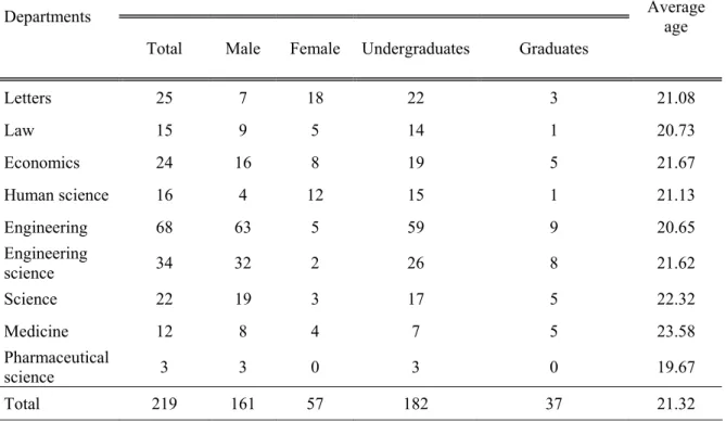
Table 1 provides some information about our subjects. As for age, subjects are 18 to 37 years of age, but most of them are around 20 years old. Among 219 subjects, 26% are female and 17% are graduate students. Subjects are well-diversified over nine departments of Osaka University.3
2.2 Procedure
2 Benzion et al. (1989) experimented with 282 students, but they did not reward the subjects. 3 No subjects are from the department of dentistry.
Each subject is required to choose one of the two options displayed on a computer screen in front.4 One is option A wherein subjects get smaller reward earlier, and the other is option B in which subjects get larger rewards later.
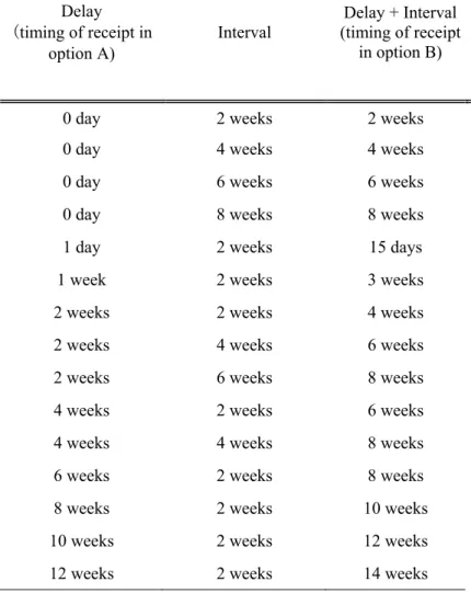
As noted in the previous sections, we control three factors: the amount of reward, interval, and delay. We define the delay as the difference between the present (time 0) and the time of receipt stated in the option A, and specify eight different delays. We define the interval as the difference between the time of receipt stated in the options A and B, and specify four intervals. Pairing these delays and intervals, we specify 15 combinations of receipt timing shown in Table 2.
We define the amount of reward as the amount stated in the option A; 180 different amounts are generated randomly from the truncated normal distribution with the mean of 2000; standard deviation of 1000; upper bound of 4000; and lower bound of 500. These 180 amounts are randomly assigned to each question. Twelve rates of return (1%, 2%, 3%, 4%, 5%, 7.5%, 10%, 12.5%, 15%, 25%, 35%, and 50%) are also randomly assigned to 12 questions of each combination. The amount of reward stated in the option B is calculated by adding the amount of reward tantamount to the above rates of return to the amount in the option A.
Thus, there are 15 combinations of receipt timing in the options A and B as shown in Table 2, and we ask 12 questions for each combination, each of which is specified with different rates of return ranging from 1% to 50%. Consequently, subjects are requested to answer 180 questions. These 180 questions are determined in advance, and all subjects answer the same questions. However, the order that the questions are presented to subjects is randomly determined for each subject.
Subjects are paid 2000 yen in cash for participation in the experiment. At the end of the
experiment, we randomly select one question out of the 180 questions, for which we will actually pay the reward. Subjects will receive a reward, a gift voucher from amazon.co.jp, on the date stated in the option they have chosen in this selected question.
2.3 Estimation of Time Discount Rates
We estimate 15 per-period time discount rates per subject, each of which corresponding to each combination of time of receipt. The procedure of the estimation is as follows. As noted in the previous subsection, 12 questions are asked for each combination of receipt timing, changing the rate of return. The answers for these 12 questions, A or B, were sorted in ascending order as per the rates of return implied by the options. If a subject chooses the option A when the rate of return is low and option B when it is high, so that they switch from the option A to B only once, then we determine the time discount rate of the subject as an average of the two rates of return immediately before and after the switch.
However, some subjects made two or more switches between the two options during answering of the 12 questions with the same combination of the receipt timing.5 This is
probable because the questions were asked randomly. In such a multi-switching case, we estimate the time discount rates using a logit model. Specifically, the dependent variable is a dummy variable that takes unity when a subject chooses B (later option) and zero otherwise, and is regressed over the 12 rates of return. Then, using the estimates of the coefficient, we calculate back a rate of return where a probability of choosing B becomes just 0.5, and regard it as the time discount rate of the subject for this combination of receipt timing. We exclude the data from our analyses if the estimated time discount rates using the logit model are out of the 1% to 50% range. Moreover, if a subject consistently chooses A (or B) for 12 questions of
5 1,352 out of 3,285 time discount rates (219 subjects × 15 combinations of receipt timings) fall into
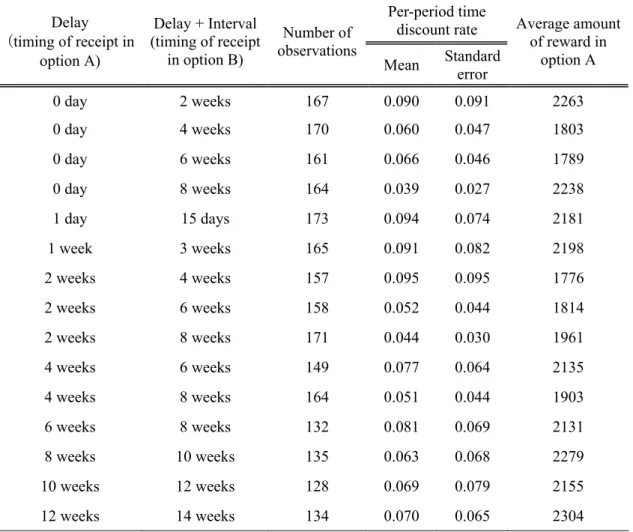
the same combination of receipt timings, we exclude those observations from our analyses.6 In this paper, we denote the subjects’ time discount rates between time a and b calculated by the above procedure as β(a,b), and the corresponding per-period time discount rate R(a,b), where the unit period is set at two weeks.7 In Table 3, we show the number of observations, the mean and the standard deviation of per-period time discount rates, and the mean of the amount of reward for each combination of receipt timing.
3.
Results
3.1 Declining Impatience
To confirm that the per-period time discount rates are diminishing with the delay, we choose the combinations in which the delays are different but the intervals are the same, and compare their discount rates.8 In other words, we select the observations of the same interval and examine whether there exists a negative correlation between the delay and the time discount rate within these observations.
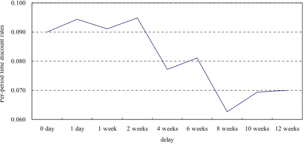
Let us first analyze the case where the interval is set at two weeks. Figure 1, which depicts the relation of the per-period time discount rates (vertical axis) and the delay (horizontal axis), reveals that the per-period time discount rate tends to decline as the delay increases, keeping the interval at two weeks. While the discount rates are in a range from 0.090 to 0.095 when the delay is within two weeks, they are less than 0.085 on and over a four-week delay, suggesting that the per-period time discount rates shift downward during the
6 957 out of 3,285 observations are excluded; 625 (43 respectively) observations are excluded because
subjects chose B (A) for all questions; 289 observations are excluded because the time discount rates estimated by the logit model are not in the range from 1% to 50%.
7 For example, the value of
) 4 , 0 (
1+R day weeks is calculated as the square root of 1+β(0day,4weeks), and the value of 1+R(0day,6weeks) is calculated as the cube root of 1+β(0day,6weeks).
8 We cannot control the amount of reward because it is randomly chosen for each question. As shown
in the far-right column of Table 3, however, the average amounts do not differ substantially among 15 combinations of receipt timing. Therefore, possible biases due to the uncontrolled amount may be trivial.
two- to four-week delay.
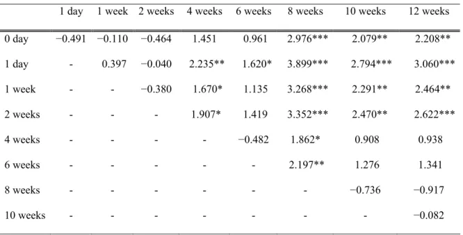
To examine its significance, we pick up observations whose intervals are the same and conduct a mean-difference test among groups with different delays. The test results are shown in Table 4, which reveals that the discount rates within a two-week delay are significantly different from those over a four-week delay. In addition, the discount rates within a two-week delay are not significantly different from each other, and the discount rates over a four-week delay seldom differ significantly from each other. These results suggest that the per-period time discount rates with a two-week interval substantially decrease during a two- to four-week delay.
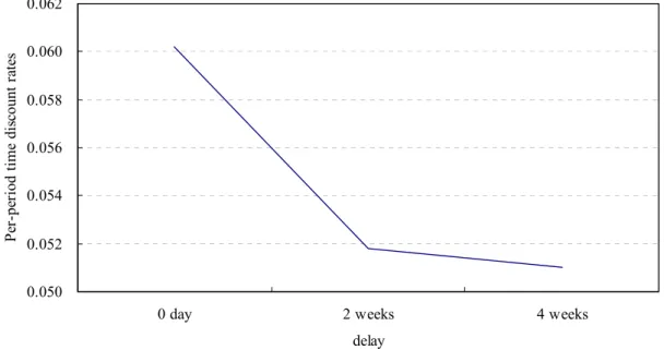
Figure 2 depicts the relationship between the per-period time discount rates and the delay, with the interval being kept at four weeks. Table 5 presents the result of the mean-difference tests for the case of a four-week interval. Although there is no significant difference between the per-period time discount rate with a two-week delay and that with a four-week delay, the per-period time discount rate with zero-day delay is significantly different from the per-period time discount rates with two- and four-week delays. These results confirm the declining impatience between the zero-day and two-week delays, for the case of a four-week interval.
When the interval is fixed at six weeks, the average time discount rate of the zero-day delay )R(0day,6weeks is 0.066, while that of the two-week delay R(2weeks,8weeks) is 0.044; the latter is significantly lower than the former (t-value is 4.948). This indicates that the per-period time discount rates also diminish with the delay in the case of the six-week interval. In sum, declining impatience is recognized during the shorter delays irrespective of the interval.
3.2 Regression Analysis with Panel Data
In the previous subsection, we conducted mean-difference tests keeping the intervals fixed and found declining impatience. In this subsection, we run a regression to confirm declining impatience controlling the magnitude effect and subjects’ attributes in addition to the interval effect. The analysis will elucidate how time discount rates depend on the delay, interval, amount of reward, and attributes of the subjects.
Specifically, we regress the panel data of the per-period time discount rates of 3285 observations (i.e., 219 subjects × 15 combinations of receipt timing) on experimental conditions (the delay, interval, and amount of reward) and subjects’ attributes (gender, age, and their affiliated department).9 This analysis has an advantage of comprehensive use of the experimental results.
The following variables of experimental conditions and attributes of subjects are employed in the estimation: eight dummy variables for delay, taking the zero-day delay as a benchmark; three dummy variables for the interval, taking the two-week interval as a benchmark; and the average amount of reward that is defined as the average of the amount of reward of 12 questions in the same combination of receipt timing.10 As for subjects’ attributes,
we employ a male dummy variable for gender, age, a dummy variable standing for graduates, and eight dummy variables standing for each department, taking the department of engineering as the reference group.
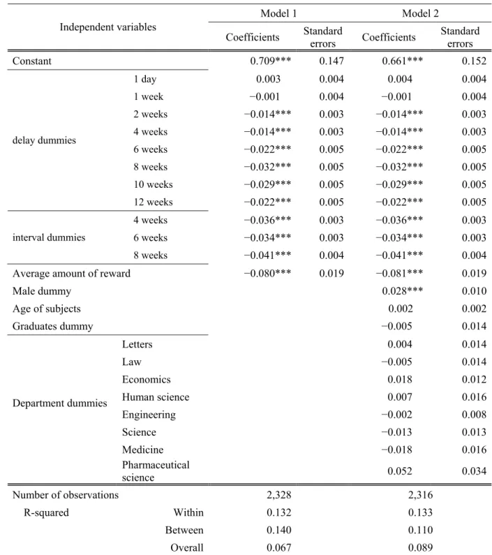
The regression results are presented in Table 6. Model 1 is a regression which considers only experimental conditions, while Model 2 stands for a regression which incorporates subjects’ attributes into Model 1. The results of Model 1 reveal that although one-day and one-week delays do not affect significantly, the longer delay dummies have significant
9 Subjects’ attributes are based on the questionnaire survey conducted at the end of the experiment. 10 We use the average of 12 amounts of reward because it is hard to identify the amount of reward
corresponding to the dependent variable, especially in the case where the time discount rate is estimated by a logit model.
negative effects. In addition, the coefficients of the dummies keep decreasing until the eight-week delay. These results imply that the declining impatience is observed even when the effect of the amount of reward as well as the interval is controlled.
All the intervals have significant negative coefficients, supporting the interval effect that the per-period time discount rate is diminishing with the interval. Closer inspection reveals that it may decrease monotonically if we evaluate the coefficients of four- and six-week intervals as similar.
The average amount of reward has a significantly negative coefficient, indicating the magnitude effect wherein the larger the amount of reward, the lower the per-period time discount rate.
When the attribute variables are added (see Model 2), the coefficients of the delay and interval dummies and the average amount of reward are almost unchanged, implying that the above results are fairly robust.
The male dummy has a significant positive coefficient, indicating male is more impatient than female, as Ikeda et al. (2005) report. As for the age, Ikeda et al. (2005) report that the older subjects tend to have lower per-period time discount rates; however, this age effect is not confirmed in our experiment. This may be because most of our subjects are around 20 years old, while the age of their subjects spreads over a wide range. All the department dummies, taking the department of engineering as the benchmark, did not have significant coefficients, although departments of medicine and science are relatively low and departments of economics and pharmaceutical science are high. When we set the department of economics as the reference group, however, a dummy representing the department of medicine has a significantly negative coefficient, indicating that students of the department of medicine are more patient than those of the department of economics.
3.3 Subadditive Time Discounting
As noted in section 1, time discounting is subadditive if the interval effect exists. Therefore, the results of the interval effect presented in the previous subsection imply that the time discounting should be subadditive. In this subsection, we directly confirm that the time discounting of our subjects is actually subadditive.
We denote the time discount rate (plus unity) between time a and time b, for the case where the period is not divided, as U (a, b). This corresponds to the left-hand side of inequality (2). Meanwhile, we denote the same time discount rate (plus one), for the case where the period is divided into n subintervals, as D (n, a, b). Specifically, D (n, a, b) is defined as the product of the time discount rates of the subintervals, which corresponds to the right-hand side of inequality (2). In this subsection, we use the time discount rates for various periods instead of the per-period one for the sake of simplicity of notation.
While Read (2001) divides the total intervals of 18 months and 24 months into three equal-length subintervals for the test of the subadditivity, we employ various shorter total intervals of four, six, and eight weeks, and divide them into shorter subintervals such as two weeks. While Read (2001) examines the case of three divisions, we also test two and four divisions, as well as three, to see the robustness of the subadditivity.
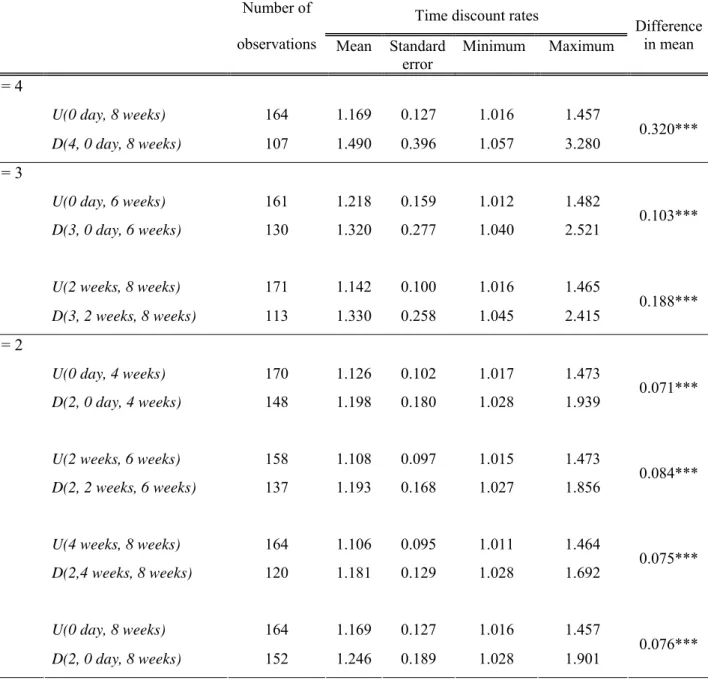
Table 7, which presents the results on the subadditivity, reveals that the time discount rates in the divided cases are significantly higher than those of the undivided cases irrespective of the number of divisions. As expected, the subadditive time discounting is observed in our experiment as in Read (2001). Furthermore, since U (0 day, 8 weeks) < D (2, 0 days, 8 weeks) < D (4, 0 days, 8 weeks), we conclude that the subadditivity is stronger as the number of divisions is larger.
Division is a kind of shortening of an interval, and the interval effect is a sufficient condition for the subadditivity as explained in section 1. Thus, it is no surprise that we
observe the subadditive time discounting, because we have already found the interval effect. In addition, since the larger number of divisions implies shorter intervals, the result in which the subadditivity for a larger number of divisions is stronger is also consistent with the interval effect.11
4.
Robustness Check with Survey Data
In this section, we check the robustness of the declining impatience observed in our experiment by analyzing the results of a questionnaire survey conducted at the end of the experiment. In our experiment, subjects are requested to answer 180 questions presented in random order. This randomness of presentation might cause bias. On the other hand, in the questionnaire survey, subjects are asked two questions. Which one do they prefer: (A) 10,000 yen in two days or (B) X yen in nine days; and the other is between (A) 10,000 yen in 90 days or (B) Y yen in 97 days. Eight values are assigned for Xs and Ys in these questions.12 Because both questions differ only in the delay and their interval and amount of reward are the same, we can test the declining impatience by just comparing the responses to both the questions. The largest difference from the questions asked in the experiment is that these questions are aligned in ascending order of X and Y, and subjects can read all eight questions before they answer. Therefore, subjects’ choice may depend on these eight questions. In addition, the questionnaire survey is also different from the experiment in that subjects are not paid a reward based on their choices.
As in the case of the experiment, we determine time discount rates of the subjects at the
11 Of course, this paper does not dismiss the possibility that the subadditivity is caused by some
additional factors to the interval effect. For instance, when the divided and undivided cases are compared, delay is also different between the cases: while only one delay is involved in the undivided case, a couple of delays are involved in the divided case. In addition, it might be the case that division itself affects the time discount rate. However, this paper does not pursue how the subadditivity is different from the interval effect. To elucidate this point, it is necessary to devise specific experiments, which will be a future task.
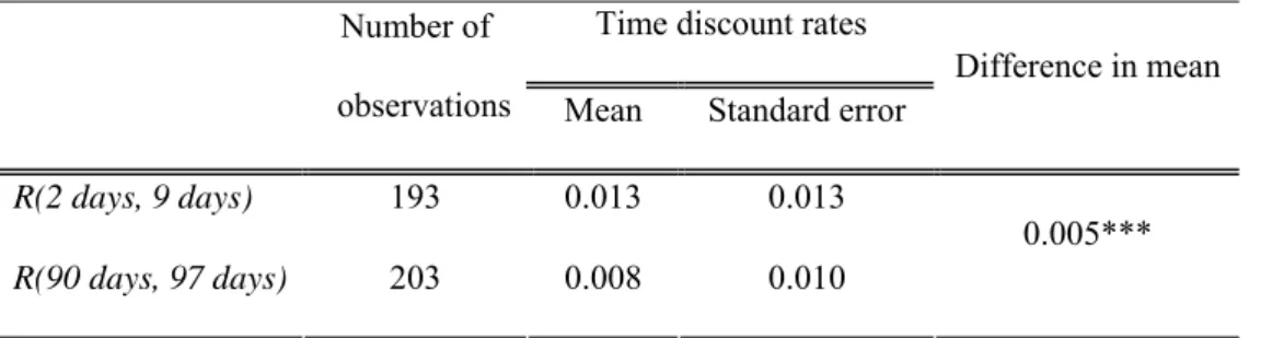
average of the two rates of return immediately before and after a switch.13 The result of the mean-difference test is shown in Table 8, which reveals that the mean of subjects’ per-period time discount rates in the questionnaire is substantially lower than the corresponding figure in the experiment shown in Table 3. For example, R(2 days, 9 days) is 0.013 in Table 8, while R(1 day, 15 days) is 0.094 in Table 3. This discrepancy arises probably because the amount of reward in the questionnaire is about five times larger than that in the experiment.
Table 8 reveals that the discount rate of a two-day delay is significantly higher than that of a 90-day delay, implying that the declining impatience is also observed in the answers to survey questions. In sum, the results of the declining impatience is robust depending on whether the questions are presented one by one in random order or simultaneously in ascending order, and whether or not a reward is paid depending on their choice.
5.
What Causes the Anomalies?
5.1 Traditional Assumption and Time Discounting Anomalies
This paper confirms three anomalies: the declining impatience and interval and magnitude effects. This section pursues the reason why these anomalies occur.
When subjects consider which is preferable, (A) receive X yen at time s or (B) receive Y yen at time t, information on the amount of reward in the two options X and Y and that on timing of receipt in the two options s and t are at hand. Traditional economics, however, assumes that people are rational, so that they have their own per-period time discount rate, ˜ R , a priori, and compare ˜ R with the rate of return, R, calculated from the four pieces of information as ( ) 1 1 − ⎟ ⎠ ⎞ ⎜ ⎝ ⎛ = −s t X Y R (5)
13In this analysis, we regard multi-switching cases as irrational choices and exclude them from the
to determine their choices. The four pieces of information are condensed into the rate of return, R, and only R is compared with ˜ R to determine the subjects’ decision on the earlier or later options; no other information has additional effect on their decision. As we observed in previous sections, such assumption evidently does not match with the reality. Time discount rate, ˜ R , of the people is not a constant but is dependent on the experimental conditions of each question, X, Y, t, and s. In other words, subjects’ time discount rates, ˜ R , depend on the delay, interval, and amount of reward; and the choice of people is not determined only by the rate of return, R, implied in the two options. These facts imply that the traditional assumption of a rational human being does not apply and therefore are anomalies. In this section, we examine two hypotheses that may explain these anomalies.
5.2 Differential Effect Hypothesis
In this subsection, we examine a reason why the interval and the amount of reward affected subjects’ decision-making in addition to the rate of return, R. Specifically, we propose a hypothesis that subjects are affected by a differential in amount (hereafter, differential effect hypothesis) as a source of the interval and magnitude effects and test it. Since the differential in amount is described as ( ) 1] ) 1 [( + − × = − t−s R X X Y , (6)
it increases as the length of the interval and the amount of reward increase. If our subjects make a decision based on the differential in amount, subjects choose the later option when the interval becomes longer or the amount of reward gets larger, even though the rate of return does not change. Consequently, when the differential in amount of reward is large, subjects report lower discount rate, so that we will find negative coefficients on the intervals and on the amount of reward when discount rates are regressed over these variables. This is actually what we observed in Table 6. If this differential effect hypothesis is true, we expect that
coefficients on the interval and the amount become larger when the variable of the differential is added to this regression.
However, this regression is problematic because, as noted in footnote 10, it is difficult to identify the amount (therefore, the differentials also) corresponding to the time discount rate estimated by a logit model. To solve this problem, we regress subjects’ binary choices on the earlier or later option over the four experimental conditions, instead of the two-step method in which we estimate discount rate at the first step, and then explain it with the experimental conditions in the second step. The method in this section has an advantage of the efficient use of all the information from 180 choices per subject. More importantly, while the two-step method premises that subjects make a decision based only on their specific per-period time discount rate, R~, the current method has no need of such a premise that was already found incorrect.
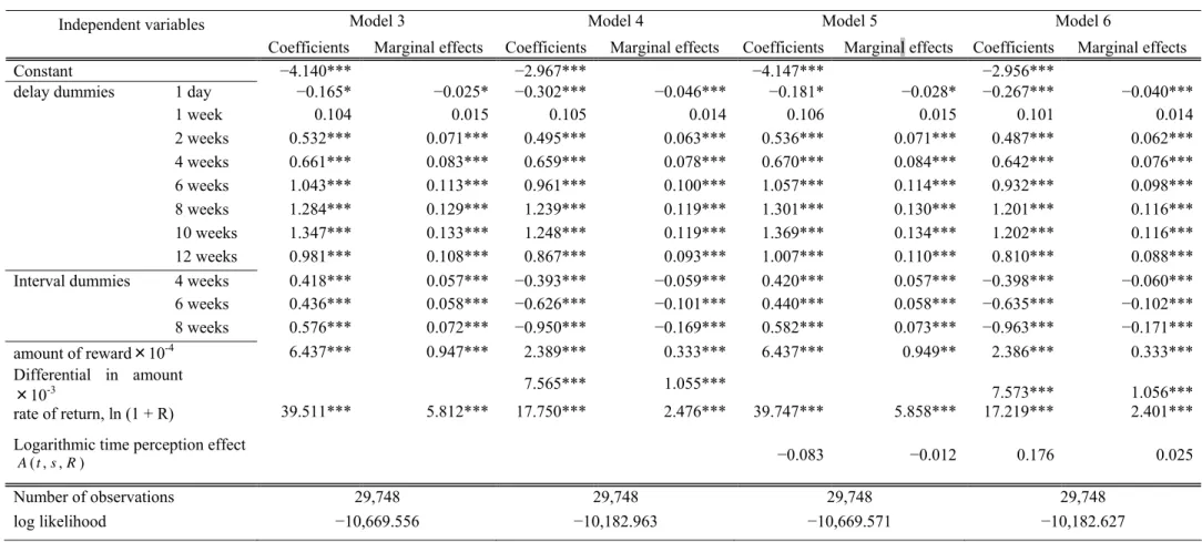
We regress the dependent variable, a dummy variable that takes unity in case a subject chooses the later option and zero otherwise, over dummy variables standing for each delay, dummy variables for each interval, the amount of reward, and logarithm of the per-period rate of return, ln(1+R) . The estimation results of this specification (Model 3), as well as the specification (Model 4) that incorporates the differential in amount as an independent variable, are presented in Table 9.14 The estimation method is a panel logit cum random effect model.
Let us examine the results of Model 3 first. The rate of return has a significantly positive coefficient, implying that the rate of return is an important factor in decision-making, as traditional economics assumes. However, the rate of return is not the only factor which solely determines the intertemporal choice. In addition to the rate of return, the delay has an additional explanatory power. The dummy variables for the delays, except for those representing a one-day delay and a one week-delay, have significant positive coefficients and
14 Four variables out of these five explanatory variables determine the remaining one variable.
become larger for longer delays. In short, subjects tend to choose the later options as the delay is larger, even when the rate of return is controlled. This fact is the counterpart to the declining impatience reported in Table 6, because the result that subjects choose the later option as the delay is getting extended indicates that the switch from the earlier option to the later option occurs at a lower discount rate, as the delay is larger. This in turn implies that lower per-period time discount rates are found as the delay is extended.
The interval dummies are also significantly positive, implying that subjects increasingly choose the later options, as the interval extends. This fact corresponds to the interval effect observed in Table 6.
The coefficient of the amount of reward is also significantly positive, implying that subjects tend to increasingly choose the later option as the amount of reward increases. The result corresponds to the magnitude effect observed in Table 6.
Now, let us turn to Model 4 that incorporates the differential in amount as an explanatory variable. Compared with Model 3, the marginal effects of the interval dummies change their signs from significantly positive to significantly negative, while those of the delay dummies are unchanged. The marginal effect of the amount of reward also becomes smaller to about one-third of the case of Model 3. These results support our hypothesis that the interval and the amount of reward affect subjects’ choice via a change in the differential in amount. In other words, the interval and the magnitude effects are caused by the differential effect at least partially.
How strong is the differential effect? The coefficient of the differential in amount is significantly positive, which means that subjects increasingly choose the later option as the differential increases. Its marginal effect is 1.055 × 10⁻³. On the other hand, when the differential is added to the regression, the marginal effect of the rate of return decreases to 2.476, about two-fifth of Model 3. These values of the marginal effects imply that a 1%
increase in the logarithm of rate of return and a 20-yen increase in the differential in amount will cause nearly the same increase in the probability of choosing the later option.15 Thus, a change in the differential in amount has a comparable effect on the subjects’ choice as a change in the rate of return.
As possible causes of subadditivity, Read (2001) pointed out a psychological effect of focusing stronger attention to smaller intervals when they are divided (support theory), and a bias toward the midpoint in subjective estimates leading to overestimates of small quantities (regression effect). This paper argues that the differential effect may be an additional cause of the interval effect. Table 9 suggests that once the differential effect is adjusted, the remaining interval effect is that subjects increasingly choose the earlier option as interval gets longer, which is the opposite of the total interval effect.
5.3 Weber’s Law
Many psychophysicists have traditionally considered that people perceive external stimulus (e.g., loudness) after transforming them by a nonlinear function. This is called Weber’s law. Recent studies further suggest that time perception also follows Weber’s law (Takahashi, 2005, 2006; Dehaene, 2003; Okamoto and Funaki, 2001). In short, relationship between objective and subjective times is nonlinear. Weber’s law gives us another hypothesis that may explain anomalies on intertemporal choice. Takahashi (2005) argues that hyperbolic time discounting function is derived from exponential discounting and Weber’s law. In other words, if time perception follows Weber’s law, people show declining impatience even if they discount future reward exponentially. In addition, Takahashi (2006) shows that the interval effect may be explained by the exponential discounting and Weber’s law. In this section, we
15 The results that use the rate of return
R instead of ln (1+R) may better appeal to our intuition. The
estimation results are almost the same as those of Model 3 in Table 9, which imply that a 1% increase in the rate of return and a 16-yen increase in the differential in amount will cause nearly the same increase in the probability of choosing the later option.
empirically investigate whether or not both anomalies are really dissolved by Weber’s law. Following Takahashi (2005), we define subjective time as logarithm of objective time (logarithmic time perception).
τ ≡αln(1+t), (7)
where τ stands for subjective time, while t is objective time, and α is a parameter. Let us describe how the rate of return is perceived by a subject with logarithmic time perception. The rate of return of a reward, R, in the experiments is defined as (5), where t and s are objective time. However, if the subject perceives time as transformed by (7), he or she feels the rate of return of the reward as Rˆ , which is defined as
) 1 ln( 1 ) , , ( ) 1 ln( 1 ) 1 ln( ) 1 ln( ) 1 ln( ) ˆ 1 ln( R R s t A R R s t s t R + + ≡ + + + + − + − = + α α . (8)
Thus, the claim by Takahashi (2005, 2006) is examined by testing whether or not the delay and the interval terms become insignificant, when the rate of return R is replaced with the perceived rate of return Rˆ in Model 3 of Table 9. The replacement is actually an addition of the term A(t,s,R) of (8) to Model 3, since the second term is nothing but ln(1+R). If the logarithmic time perception model is correct, A(t,s,R) has significant effect on the subject’s choice.
The estimation results of this regression (Model 5) are presented in the right columns of Table 9. The first term of (8), which we denote as A(t,s,R) in Table 9, is not significant at all; and the coefficient of the second term, ln(1+R), is not different from that of Model 3. The coefficients of the delay and the interval dummies are significant and their values are almost the same as those of Model 3. In sum, the logarithmic time perception hypothesis does not solve the anomalies on the delay and interval.
does not bring about additional explanatory power, suggesting that objective time better explains the choice of the binary options than the logarithmic time perception hypothesis.
Finally, let us confirm whether the differential effect hypothesis is supported even though Weber’s law is considered. In the far-right column, the estimation results that both
) , , (t s R
A and the differential in amount are included in the regression are shown (Model 6). The results are almost the same as those of Model 4, so that the conclusion of the previous subsection is retained.
6. Conclusion
This paper examined the effects of the delay and interval on the subjects’ time discount rates, as well as the effect of the differentials in amount of reward on the subjects’ choice, using the result of an experiment on time discount rates and a questionnaire survey conducted together with the experiment. Thus far, most of the researches did not distinguish the delay from the interval, so that whether the decreasing impatience really holds has been an open question. We conducted an experiment that explicitly distinguished the delay from the interval, and found that per-period time discount rates keep decreasing up to the eight-week delay when the interval is controlled. This implies that people make dynamic inconsistent plans and show a preference reversal.
This paper also focused on whether time discount rates depend on the interval between the two options. Although this problem has seldom been investigated, we found the interval effect in which the per-period time discount rate decreases as the interval lengthens. This interval effect is a sufficient condition for subadditive time discounting proposed by Read (2001), and we confirmed the subadditivity under different conditions. Finally, we found that the interval and the magnitude effects are caused, at least partially, because subjects’ choice are influenced by the differential in reward amount, while Weber’s law does not solve the
delay nor the interval effects.
While many previous studies propose various functional forms of time discounting, our results above suggest that any of them are insufficient to cover the experimental facts. Hyperbolic and quasi-hyperbolic discounting functions proposed by Loewenstein and Prelec (1992) and Laibson (1997) depend only on the delay, and ignore the interval. Therefore, they cannot explain the interval effect observed in our experiment. Read (2001) proposed a functional form, which considers the interval effect (subadditivity, in his words) but disregards declining impatience. However, the results of this paper call for a discounting function, which properly explains both the declining impatience and the interval effect.
References
Benzion, Uri, Amnon Rapoport, and Joseph Yagil. (1989). Discount Rates Inferred from Decisions: An Experimental Study, Management Science, 35, 270–284.
Dehaene, Stanislas. (2003). The Neural Basis of the Weber–Fechner law: A Logarithmic Mental Number Line, TRENDS in Cognitive Sciences, 7, 145–7.
Fischbacher, Urs. (1999). Z-Tree: A Toolbox for Readymade Economic Experiments, IEW Working paper 21, University of Zurich.
Frederick, Shane, George Loewenstein, and Ted O’Donoghue. (2002). Time Discounting and Time Preference: A Critical Review, Journal of Economic Literature, 40, 351–401.
Green, Leonard, Joel Myerson, and Edward McFadden. (1997). Rate of Temporal Discounting Decreases with Amount of Reward, Memory & Cognition, 25, 715–723.
Ikeda, Shinsuke, Fumio Ohtake, and Yoshiro Tsutsui. (2005). Time Discount Rates: An Analysis Based on Economic Experiments and Questionnaire Surveys, Institute of Social and Economic Research Discussion Paper, 638, 1–36 (in Japanese).
Kirby, Kris N., and Nino N. Marakovic. (1995). Modeling Myopic Decisions: Evidence for Hyperbolic Delay-Discounting within Subjects and Amounts, Organizational Behavior and Human Decision Processes, 64, 22–30.
Laibson, David. (1997). Golden Eggs and Hyperbolic Discounting, Quarterly Journal of Economics, 112, 443–477.
Loewenstein, George, and Drazen Prelec. (1992). Anomalies in Intertemporal Choice: Evidence and an Interpretation, Quarterly Journal of Economics, 107, 573–597.
Myerson, Joel, and Leonard Green. (1995). Discounting of Delayed Rewards: Models of Individual Choice, Journal of The Experimental Analysis of Behavior, 64, 263–276.
Okamoto, Hiroshi, and Tomoki Fukai. (2001). Neural Mechanism for a Cognitive Timer, Physical Review Letters, 86, 3919–22.
Pender, John L. (1996). Discount Rates and Credit Markets: Theory and Evidence from Rural India, Journal of Development Economics, 50, 257–296.
Read, Daniel. (2001). Is Time-Discounting Hyperbolic or Subadditive? Journal of Risk and Uncertainty, 23, 5–32.
Richards, Jerry B., Lan Zhang, Suzanne H. Mitchell, and Harriet De Wit. (1999). Delay or Probability Discounting in a Model of Impulsive Behavior: Effect of Alcohol, Journal of The Experimental Analysis of Behavior, 71, 121–143.
Takahashi, Taiki. (2005). Loss of Self-control in Intertemporal Choice may be Attributable to Logarithmic Time-perception, Medical Hypotheses 65, 691–63.
Takahashi, Taiki. (2006). Time-estimation Error Following Weber-Fechner Law May Explain Subadditive Time-discounting, Medical Hypotheses 67, 1372–74.
Thaler, Richard. (1981). Some Empirical Evidence on Dynamic Inconsistency, Economic Letters, 8, 201–207.
Uzawa, Hirofumi. (1968). Time Preference, the Consumption Function and Optimum Asset Holdings, in: J.N. Wolfe, ed., Value Capital and Growth: Papers In Honour of Sir John Hicks (Chicago: Aldine).
Table 1 Attributes of subjects
Number of subjects Departments
Total Male Female Undergraduates Graduates
Average age Letters 25 7 18 22 3 21.08 Law 15 9 5 14 1 20.73 Economics 24 16 8 19 5 21.67 Human science 16 4 12 15 1 21.13 Engineering 68 63 5 59 9 20.65 Engineering science 34 32 2 26 8 21.62 Science 22 19 3 17 5 22.32 Medicine 12 8 4 7 5 23.58 Pharmaceutical science 3 3 0 3 0 19.67 Total 219 161 57 182 37 21.32
Table 2 Fifteen combinations of receipt timing in earlier and later options Delay (timing of receipt in option A) Interval Delay + Interval (timing of receipt in option B)
0 day 2 weeks 2 weeks
0 day 4 weeks 4 weeks
0 day 6 weeks 6 weeks
0 day 8 weeks 8 weeks
1 day 2 weeks 15 days
1 week 2 weeks 3 weeks
2 weeks 2 weeks 4 weeks
2 weeks 4 weeks 6 weeks
2 weeks 6 weeks 8 weeks
4 weeks 2 weeks 6 weeks
4 weeks 4 weeks 8 weeks
6 weeks 2 weeks 8 weeks
8 weeks 2 weeks 10 weeks
10 weeks 2 weeks 12 weeks
Table 3 Per-period time discount rates Per-period time discount rate Delay (timing of receipt in option A) Delay + Interval (timing of receipt in option B) Number of observations
Mean Standard error
Average amount of reward in option A 0 day 2 weeks 167 0.090 0.091 2263 0 day 4 weeks 170 0.060 0.047 1803 0 day 6 weeks 161 0.066 0.046 1789 0 day 8 weeks 164 0.039 0.027 2238 1 day 15 days 173 0.094 0.074 2181 1 week 3 weeks 165 0.091 0.082 2198 2 weeks 4 weeks 157 0.095 0.095 1776 2 weeks 6 weeks 158 0.052 0.044 1814 2 weeks 8 weeks 171 0.044 0.030 1961 4 weeks 6 weeks 149 0.077 0.064 2135 4 weeks 8 weeks 164 0.051 0.044 1903 6 weeks 8 weeks 132 0.081 0.069 2131 8 weeks 10 weeks 135 0.063 0.068 2279 10 weeks 12 weeks 128 0.069 0.079 2155 12 weeks 14 weeks 134 0.070 0.065 2304
Notes: Table shows the number of observations, mean and standard deviation of per-period time discount rates, and the average of the amount of reward for each combination of receipt timing. The number of observations is less than the number of subjects, 219, because we exclude the observations if a subject consistently chooses A (or B) for 12 questions of the same combination, and that the estimated time discount rates using a logit model are out of the 1% to 50% range.
Table 4 Test results for the declining impatience for the case that the interval is held at 2 weeks
1 day 1 week 2 weeks 4 weeks 6 weeks 8 weeks 10 weeks 12 weeks 0 day −0.491 −0.110 −0.464 1.451 0.961 2.976*** 2.079** 2.208** 1 day - 0.397 −0.040 2.235** 1.620* 3.899*** 2.794*** 3.060*** 1 week - - −0.380 1.670* 1.135 3.268*** 2.291** 2.464** 2 weeks - - - 1.907* 1.419 3.352*** 2.470** 2.622*** 4 weeks - - - - −0.482 1.862* 0.908 0.938 6 weeks - - - 2.197** 1.276 1.341 8 weeks - - - −0.736 −0.917 10 weeks - - - −0.082
Notes: Observations whose interval is 2 weeks are picked up and a mean-difference test among groups with different delays is applied. The figures in each cell are t-values for the mean-difference test between per-period time discount rates of two groups with different delays shown in the first column and the first row; ***, **, and * indicate that the values are statistically significant at the 1%, 5% , and 10% levels, respectively.
Table 5 Test results for the declining impatience for the case that the interval is held at 4 weeks
2 weeks 4 weeks 0 day 1.663* 1.857*
2 weeks 0.167
Notes: Observations whose interval is 4 weeks are picked up and a mean-difference test among groups with different delays is applied. The figures in each cell are t-values for the mean-difference test between per-period time discount rates of two groups with different delays shown in the first column and the first row; * indicates that the values are statistically significant at the 10% level.
Table 6 Regression results of per-period time discount rates on experimental conditions and attributes of subjects
Model 1 Model 2
Independent variables
Coefficients Standard errors Coefficients Standard errors
Constant 0.709*** 0.147 0.661*** 0.152 1 day 0.003 0.004 0.004 0.004 1 week −0.001 0.004 −0.001 0.004 2 weeks −0.014*** 0.003 −0.014*** 0.003 4 weeks −0.014*** 0.003 −0.014*** 0.003 6 weeks −0.022*** 0.005 −0.022*** 0.005 8 weeks −0.032*** 0.005 −0.032*** 0.005 10 weeks −0.029*** 0.005 −0.029*** 0.005 delay dummies 12 weeks −0.022*** 0.005 −0.022*** 0.005 4 weeks −0.036*** 0.003 −0.036*** 0.003 6 weeks −0.034*** 0.003 −0.034*** 0.003 interval dummies 8 weeks −0.041*** 0.004 −0.041*** 0.004
Average amount of reward −0.080*** 0.019 −0.081*** 0.019
Male dummy 0.028*** 0.010 Age of subjects 0.002 0.002 Graduates dummy −0.005 0.014 Letters 0.004 0.014 Law −0.005 0.014 Economics 0.018 0.012 Human science 0.007 0.016 Engineering −0.002 0.008 Science −0.013 0.013 Medicine −0.018 0.016 Department dummies Pharmaceutical science 0.052 0.034 Number of observations 2,328 2,316 R-squared Within 0.132 0.133 Between 0.140 0.110 Overall 0.067 0.089
Notes: Only the regression results from random effect model are shown because it was not rejected against fixed effect model by Hausman specification test. Dependent variable is the per-period time discount rates; *** indicates that the values are significant at the 1% level. The number of observations is less than the total observations (219 subjects × 15 combinations of receipt timing) because we exclude the observations that a subject consistently chooses A (or B) for 12 questions of the same combination, and that the estimated time discount rates using a logit model are out of the 1% to 50% range.
Table 7 Test results on the subadditive time discounting
Time discount rates Number of
observations Mean Standard error
Minimum Maximum
Difference in mean
n = 4
U(0 day, 8 weeks) 164 1.169 0.127 1.016 1.457
D(4, 0 day, 8 weeks) 107 1.490 0.396 1.057 3.280 0.320***
n = 3
U(0 day, 6 weeks) 161 1.218 0.159 1.012 1.482
D(3, 0 day, 6 weeks) 130 1.320 0.277 1.040 2.521
0.103***
U(2 weeks, 8 weeks) 171 1.142 0.100 1.016 1.465
D(3, 2 weeks, 8 weeks) 113 1.330 0.258 1.045 2.415
0.188***
n = 2
U(0 day, 4 weeks) 170 1.126 0.102 1.017 1.473
D(2, 0 day, 4 weeks) 148 1.198 0.180 1.028 1.939
0.071***
U(2 weeks, 6 weeks) 158 1.108 0.097 1.015 1.473
D(2, 2 weeks, 6 weeks) 137 1.193 0.168 1.027 1.856 0.084***
U(4 weeks, 8 weeks) 164 1.106 0.095 1.011 1.464
D(2,4 weeks, 8 weeks) 120 1.181 0.129 1.028 1.692
0.075***
U(0 day, 8 weeks) 164 1.169 0.127 1.016 1.457
D(2, 0 day, 8 weeks) 152 1.246 0.189 1.028 1.901
0.076***
Notes: U (a, b) denotes the time discount rate (plus one) of the undivided case between time a to b. D (n, a, b) denotes the time discount rate (plus one) of the divided case between time a to b; n
represents the number of subintervals of equal length; *** indicates that the difference in mean is significant at the 1% level.
Table 8 Test results on the declining impatience using the questionnaire survey
Time discount rates Number of
observations Mean Standard error
Difference in mean
R(2 days, 9 days) 193 0.013 0.013
R(90 days, 97 days) 203 0.008 0.010
0.005***
Notes: R(2 days, 9 days) stands for per-period time discount rate with two-day delay and seven-day
interval. R(90 days, 97days) stands for per-period time discount rate with 90-day delay and seven-day
interval. The number of observations is less than the number of subjects, 219, because we exclude the observations that a subject consistently chose all A or all B and those with multi-switching; *** indicates that the difference in mean is statistically significant at the 1% level.
Table 9 Results from the regression with panel data of responses to binary questions
Model 3 Model 4 Model 5 Model 6
Independent variables
Coefficients Marginal effects Coefficients Marginal effects Coefficients Marginal effects Coefficients Marginal effects
Constant −4.140*** −2.967*** −4.147*** −2.956***
delay dummies 1 day −0.165* −0.025* −0.302*** −0.046*** −0.181* −0.028* −0.267*** −0.040***
1 week 0.104 0.015 0.105 0.014 0.106 0.015 0.101 0.014 2 weeks 0.532*** 0.071*** 0.495*** 0.063*** 0.536*** 0.071*** 0.487*** 0.062*** 4 weeks 0.661*** 0.083*** 0.659*** 0.078*** 0.670*** 0.084*** 0.642*** 0.076*** 6 weeks 1.043*** 0.113*** 0.961*** 0.100*** 1.057*** 0.114*** 0.932*** 0.098*** 8 weeks 1.284*** 0.129*** 1.239*** 0.119*** 1.301*** 0.130*** 1.201*** 0.116*** 10 weeks 1.347*** 0.133*** 1.248*** 0.119*** 1.369*** 0.134*** 1.202*** 0.116*** 12 weeks 0.981*** 0.108*** 0.867*** 0.093*** 1.007*** 0.110*** 0.810*** 0.088***
Interval dummies 4 weeks 0.418*** 0.057*** −0.393*** −0.059*** 0.420*** 0.057*** −0.398*** −0.060***
6 weeks 0.436*** 0.058*** −0.626*** −0.101*** 0.440*** 0.058*** −0.635*** −0.102*** 8 weeks 0.576*** 0.072*** −0.950*** −0.169*** 0.582*** 0.073*** −0.963*** −0.171*** amount of reward×10-4 6.437*** 0.947*** 2.389*** 0.333*** 6.437*** 0.949** 2.386*** 0.333*** Differential in amount ×10-3 7.565*** 1.055*** 7.573*** 1.056*** rate of return, ln (1 + R) 39.511*** 5.812*** 17.750*** 2.476*** 39.747*** 5.858*** 17.219*** 2.401***
Logarithmic time perception effect ) , , (t s R A −0.083 −0.012 0.176 0.025 Number of observations 29,748 29,748 29,748 29,748 log likelihood −10,669.556 −10,182.963 −10,669.571 −10,182.627
Notes: Only the regression results of random effect model are shown because it is not rejected against fixed effect model by Hausman specification test. Dependent variable is the response to the binary questions; ***, **, and * indicate that the values are statistically significant at the 1%, 5%, and 10% levels, respectively. The number of observations is less than the total observations (219 subjects × 15 combinations of receipt timing) because we exclude the observations when a subject consistently chooses A (or B) for 12 questions of the same combination, and that the estimated time discount rates using a logit model are out of the 1% to 50% range.
0.060 0.070 0.080 0.090 0.100
0 day 1 day 1 week 2 weeks 4 weeks 6 weeks 8 weeks 10 weeks 12 weeks delay P er -pe ri od t im e d is count ra te s
Figure 1 Declining impatience in the case where the interval is kept at 2 weeks.
Note: The average of the per-period time discount rates for each delay designated at the horizontal axis is plotted. The interval is kept at 2 weeks.
0.050 0.052 0.054 0.056 0.058 0.060 0.062
0 day 2 weeks 4 weeks
delay P er -p er iod t im e di sc ount r at es
Figure 2 Declining impatience in the case where the interval is kept at 4 weeks.
Note: The average of the per-period time discount rates for each delay designated at the horizontal axis is plotted. The interval is kept at 4 weeks.