Should we be surprised by the unreliability of
real-time output gap estimates? Density estimates for
the Euro area
James Mitchell
∗National Institute of Economic and Social Research
This Revision: January 2005
Abstract
Recent work has found that, without the benefit of hindsight, it can prove dif-ficult for policy-makers to pin down accurately the current position of the output gap; real-time estimates are unreliable. However, attention primarily has focused on output gap point estimates alone. But point forecasts are better seen as the central points of ranges of uncertainty; therefore some revision to real-time estimates may not be surprising. To capture uncertainty fully density forecasts should be used. This paper introduces, motivates and discusses the idea of evaluating the quality of real-time density estimates of the output gap. It also introduces density forecast combination as a practical means to overcome problems associated with uncertainty over the appropriate output gap estimator. An application to the Euro area illus-trates the use of the techniques. Simulated out-of-sample experiments reveal that not only can real-time point estimates of the Euro area output gap be unreliable, but so can measures of uncertainty associated with them. The implications for policy-makers use of Taylor-type rules are discussed and illustrated. We find that Taylor-rules that exploit real-time output gap density estimates can provide reli-able forecasts of the ECB’s monetary policy stance only when alternative density forecasts are combined.
Keywords: Output gap; Real-Time; Density Forecasts; Density Forecast Com-bination; Taylor Rules
JEL Classification: E32; C53
∗Thanks to Andrew Harvey, Kostas Mouratidis, Tommaso Proietti, Simon van Norden, Ken Wallis
and Martin Weale for helpful comments. Thanks also to Yongmiao Hong for making available GAUSS code to implement his test referred to below. This paper is part of a programme of work undertaken at the National Institute of Economic and Social Research in London with the support of EUROSTAT. Mitchell also acknowledges financial support from the ESRC (Award Reference: RES-000-22-0610). Address for correspondence: James Mitchell, NIESR, 2 Dean Trench Street, Smith Square, London, SW1P 3HE, UK. Tel: +44 (0)207 654 1926. E-Mail: [email protected].
1
Introduction
Policy makers require output gap estimates in real-time.1 They do not have the luxury
of being able to wait before deciding whether the economy is currently lying above or below its trend level. They have to decide, without the benefit of hindsight, whether a given change to output in the current period is temporary or permanent, that is whether it is a cyclical or trend movement.2 Their problem can be interpreted as a forecasting
one, since these real-time output gap estimates are forecasts, in the sense that they are expectations of the output gap conditional on incomplete information. Only with the arrival of additional information, such as revised historical data and data not available at the time, do the output gap estimates eventually settle down at their “final” values.3
Recent work has found real-time or end-of-sample output gap (point) estimates to be unreliable, in the sense that there is a large and significant revision or forecasting error; see Orphanides & van Norden’s (2002) application to the US economy.4 The revisions associated with real-time estimates are considerable; indeed for the US they were found to be as large as the output gap estimates themselves. So-calleddata revisions, explained by revisions to published GDP data, were found to be less important than so-called
statistical revisions. Statistical revisions are explained by the arrival of new data helping macroeconomists, with the advantage of hindsight, better understand the position of the business cycle, and also perhaps revising what model they use to identify and estimate it. Clearly policy-makers misjudging the position of the business cycle in real-time, or in other words making poor forecasts, can lead to sub-optimal policy-decisions; e.g. see Nelson & Nikolov (2001), Orphanides (2001, 2003b) and Ehrmann & Smets (2003). The findings for the US, therefore, are worrying. Below we find that a similar picture of revisions to output gap estimates emerges when we look at the Euro area business cycle. But, should we be surprised by this unreliability? Previous work has largely over-looked this question. With a couple of exceptions to which we turn below, focus has hitherto been on the point forecast; as in the output gap is currently 2%, for example. But it is not a question of this forecast proving to be right and another forecast proving to be wrong. Point forecasts are better seen as the central points of ranges of uncertainty. A forecast of 2% must mean that people should not be surprised if the output gap turns out to be a little larger than that. Moreover perhaps they should not be very surprised if it turns out to be much larger or indeed nothing at all. Therefore, consistent with recent
1Since our focus is on the “growth” business cycle rather than the “classical” cycle the “business cycle”
and “output gap” are treated synonymously.
2In fact, in real time not only do policy makers apparently require current estimates of the output
gap but future or forecasted values; see Schumacher (2002). In this paper we concentrate on obtaining in real-time current estimates of the output gap, and their uncertainty. In any case, as we argue below, one can view obtaining real-time estimates of the (current) output gap as a forecasting exercise.
3Values are never truly final because data revisions and the arrival of new data are a continuous
process.
4This unreliability, of course, has long been appreciated qualitatively; e.g. see Morgenstern’s (1963)
discussion (p. 268) where he views the revisions typically associated with national accounts data as “casting serious doubts on the usefulness of national income figures for business cycle analysis”.
developments in the forecasting literature, it is important to provide a description of the uncertainty associated with real-time output gap estimates. Density forecasts provide a complete description of this uncertainty. Their importance can be seen by recalling that unless users of output gap estimates have symmetric, quadratic loss functions when making a decision they need to focus on not just the point estimate but the density; e.g. see Granger & Pesaran (2000). Given that the output gap is widely perceived as a leading indicator, albeit empirically perhaps a poor one, of future inflation an asymmetric inflation target implies an asymmetric loss function for the output gap.5 In such a case
the ‘optimal’ real-time estimate of the output gap need not equal the mean or conditional expectation: it can be ‘rational’ to use biased real-time estimates; e.g. see Elliott et al. (2004). Furthermore, measures of uncertainty are useful in their own right if interested in analysing and communicating, for example, risk and volatility, or the probability of a downturn.
Although previous work, such as Orphanides & van Norden (2002) and Camba-Mendez & Rodriguez-Palenzuela (2003), has provided measures of uncertainty associated with out-put gap estimates, via estimated standard errors, as indicated above focus has remained on the point estimates; the quality of real-time output gap estimates has been evaluated primarily by focusing on the degree and nature of ex post revisions to output gap point estimates.6 Typically this has involved examination, for example, both of the correlation between the real-time and final point estimates and the difference between the real-time and final estimates. When presented, measures of uncertainty have been evaluated in spe-cific ways - it has not been made explicit what defines a “good” measure of uncertainty. This can leave us unclear about the reliability of real-time output gap estimates and their uncertainty.
In this paper we provide a more general discussion of the importance of providing measures of uncertainty,via density forecasts, associated with real-time output gap point estimates.7 We explicitly relate the computation and evaluation of measures of uncertainty
associated with real-time output gap estimates to recently developed techniques from the forecasting literature. By comparison, previous work has left this relationship, at best, implicit and relied onad hoc tests. Camba-Mendez & Rodriguez-Palenzuela (2003) test if the standard error of the real-time estimates is equal to that of the final estimates using
5This holds for a linear relationship between inflation at timet+h(wherehis the forecast horizon) and
the output gap at timet. It seems sensible, and consistent with other commentators’ views, to interpret the European Central Bank’s [ECB] target of keeping annual inflation at 2% or less as an asymmetric target. Only if the ECB are equally happy with inflation at, say, 0% as at 2%, implying a uniform loss function, can their target be interpreted as symmetric.
6Other work has noted that the standard error bands around output gap estimates are often large
but not sought to evaluate the accuracy of these bands formally; e.g. see Gerlach & Smets (1999), Staiger et al. (1997) and Smets (1999). Applications, usually to the US, typically find standard errors slightly larger than 1%. This implies that an output gap point estimate must be at least±2% (assuming normality) before we can view it as statistically different from zero (at around a 95% level of significance).
7Our work builds on pioneering contributions, such as Stone et al. (1942) and Morgenstern (1963),
that look at the uncertainty of economic statistics. Morgenstern, for example, stresses the uncertainties associated with national income statistics and begins to quantify them using uncertainty bands (see Figure 10, p. 269).
what can be interpreted as a test for equal (point) forecast accuracy similar to Diebold & Mariano (1995), while Orphanides & van Norden (2002) actually use a type of Diebold-Mariano test on the second moments of the revision between real-time and final estimates to test if the variability of the revision process is consistent with what was expected ex post rather than ex ante.8 In contrast, we consider real-time (ex ante) computation of
measures of uncertainty associated with real-time estimates and methods of evaluation that have a clear interpretation and indeed a growing pedigree. The clarity derives from defining what constitutes a “good”, or even “optimal” (in some respect), density forecast. In this paper we also address an important practical problem faced by users of out-put gap estimates that is another important source of real-time outout-put gap uncertainty, namely model uncertainty. To-date there is no consensus on the appropriate output gap estimator. Various estimators are used by policy-makers and academics; these include Hodrick-Prescott filters, band-pass filters and univariate and multivariate unobserved components models. Inevitably these paint contrasting pictures as to the position of the output gap. It is not unusual to find one estimator suggesting the economy is above trend with another indicating the reverse. Our results for the Euro area are no different; see also Orphanides & van Norden’s (2002) results for the US. We consider five estimators representative of those used by applied macroeconomists and find that two suggest the output gap, according to our most recent estimates, is positive while three suggest it is negative. Similarly when looking not just at the point estimates but the whole density, we find substantial differences across the five density estimates.
This dissension across alternative (competing) estimates of the output gap will be familiar to macroeconomists. Indeed it may have contributed to anecdotal and published
8In the notation of Section 3, Camba-Mendez & Rodriguez-Palenzuela (2003) test if P
t|t = Pt|T,
where Pt|t is the variance of the real-time estimate ytC|t and Pt|T is the variance of the final estimate
yC
t|T. Note that the parameters are estimated, respectively, using current and full-sample information.
Under squared error loss, Gaussianity and both the real-time and final estimates having zero mean around some ‘true’ estimate (we could think of the final estimate as this ‘true’ estimate), this amounts to a test for equal forecast performance similar to Diebold & Mariano (1995). The hypothesis is tested using an F-test, whose appropriateness rests on certain, unstated, rather strong conditions such as no serial correlation. Orphanides & van Norden (2002), on the other hand, examine the revision Rt|T =
yC t|T −y C t|t
and test ifE(Rt|T) = 0 andE(Rt|T)2 =Pt|t−Pt|T via a Diebold-Mariano type test. The
estimator for the variance of the revision,Pt|t−Pt|T, is not computable in real-time (ex ante), however,
requiring full-sample information, T, to both derive the final or smoothed estimates and estimate the model parameters Θ on which the expression for E(Rt|T)2 given above is conditional. Nevertheless,
it is interesting to compare their statistic with one of the evaluation tests considered below. Their test statistic is: " 1 T XT t=1 yC t|T−yCt|t √ Pt|t−Pt|T 2 −1 #
→N0,2πfT(0)wheref(0) is some consistent estimate of the
spectral density of ( yCt|T−yCt|t √ Pt|t−Pt|T 2)T t=1
at frequency zero. In contrast our test for whether uncertainty is
“correctly” accounted for by the forecast [see Section 3.2] requires the scaled revision errors yCt|T−ytC|t √ Pt|t T t=1 to bei.i.d. N(0,1).
evidence that the output gap is a concept of limited empirical value.9 However we argue that any such conclusion is premature. In practice we know that policy-makers consult var-ious estimators to inform their judgement. This provides a rationale for model-averaging. We suggest that when the output gap is to be used for a specific purpose, like modelling or forecasting interest-rates or alternatively inflation, one should consider combining in-formation across these alternative estimators.10 However, while it is well established (e.g.
see Bates & Granger (1969) and Stock & Watson (2004)) that combining competing in-dividual point forecasts of the same event can deliver more accurate forecasts, in the sense of a lower root mean squared error (RMSE), little attention has been paid to the combination of forecasts and their uncertainty. Accordingly, we propose a simple method of combining information across alternative density forecasts that delivers the “optimal”
pooled or combined output gap estimator.11
The plan of the remainder of this paper is as follows. Section 2 illustrates the unrelia-bility of real-time output gap point estimates in the Euro area. Parameter uncertainty is found to be a dominant source of this unreliability. We then turn to whether we should be surprised by this unreliability. To this end, Section 3 considers how to measure the uncertainty associated with real-time estimates, and then evaluate them similarly to how point estimates are evaluated on the basis of their RMSE against the outturn. Section 4 then re-visits the simulated real-time application to the Euro area considered in Section 2. It indicates, and then evaluates, the degree of uncertainty associated with output gap estimates in real-time.
To draw out some implications of these empirical findings and introduce density fore-cast combination, Section 5 turns to examination of the effect of output gap uncertainty on prescriptions from monetary policy (Taylor-type) rules. It explains the circumstances in which uncertainty about real-time estimates should cause policy-makers to react less strongly to these data when they are more uncertain. The practical consequences of real-time uncertainty about the output gap for setting interest rates are then highlighted. We illustrate how uncertainty about real-time output gap estimates translates into un-certainty about the value of the policy instrument. This unun-certainty, about monetary policy stance, is again best represented by a density forecast. With an eye to establish-ing whether these Taylor-type rules explain the ECB’s (notional) behaviour, we evaluate
9For example in the context of forecasting inflation Orphanides & van Norden (2004) conclude that
their finding that real-time output gap estimates do not provide as good forecasts of inflation out-of-sample as benchmark models “call[s] into question the practical usefulness of the output gap concept for forecasting inflation” (Abstract).
10For example, N different output gap estimates translate (given a model relating, say, the interest
rate to the output gap) intoN forecasts of the interest rate that can then be combinedvia least-squares regression against the outturn (the interest rate); see Granger & Ramanathan (1984). If we wish to combine the N output gap estimates directly we confront the practical problem that the outturn (the ‘true’ value of the output gap) is not observed. One solution is to follow Smith et al. (1998) and combine theN output gap estimates based on the assumption that they are all noisy estimates of some common ‘true’ (but unknown) value of the output gap.
11It may also prove convenient when communicating about the output gap to focus on one (pooled)
whether the implied density forecasts for the interest rate offer a good characterisation of actual interest-rate movements.12 Conceptually this represents an important
depar-ture from existing studies that test how well Taylor rules fit the data with a focus on point estimates. One can potentially gain a misleading impression of these rules’ ex-planatory/forecasting power by ignoring uncertainty.13 Following Orphanides (2001) we
distinguish between real-time and final renditions of the policy-rule. We find that indi-vidually the five individual output gap estimators considered in Section 4, for the simple rules considered, do not in real-time provide a satisfactory representation of interest rates. Furthermore, reflecting model uncertainty, there is considerable disagreement across the five estimators as to the interest rate consistent with the policy rule. Accordingly, we pro-pose a simple method of combining information across these alternative density forecasts. The pooled or combined output gap estimator is defined as that linear combination of the individual density estimates that best explains actual interest rate movements. This combined density forecast is found to offer improved density forecasts for the Euro-area interest-rate. Section 6 offers some concluding comments. Details of the data and models used are confined to appendices.
2
The unreliability of real-time output gap point
es-timates illustrated. An application to the Euro area
Euro area data are taken from the ECB’s Area Wide Model (AWM) database; see Ap-pendix A for more details.14 It is expedient in an application to the Euro area to focus on statistical revisions alone as construction of a ‘real-time’ data set is not readily possible. We do, however, make an attempt at construction of an “approximate” real-time data set for GDP; see Appendix A.1.15 This is meant merely to be suggestive and in the main body of the paper attention is restricted to the AWM data, i.e. to statistical revisions alone, by considering what amounts to a ‘final’ data vintage.
To illustrate the unreliability of real-time output gap estimates the following
experi-12If the rule does replicate actual interest-rate movements then by using the rule as a benchmark the
ECB ensure a degree of continuity in monetary policy behaviour pre and post EMU. For a discussion of some normative aspects of these rules (e.g. how ‘good’ are they?) with a focus on the ECB see Peersman & Smets (1999).
13In a related literature, authors have argued that the failure to find empirical support out-of-sample
for nonlinear business cycle forecasts may be explained by the traditional focus on point forecasts and RMSE. They argue that nonlinear models may do better at forecasting higher moments, that are captured by density forecasts; see Clements et al. (2003).
14Related studies that examine real-time output gap estimates for the Euro area are Runstler (2002)
and Camba-Mendez & Rodriguez-Palenzuela (2003). They ignore data revisions, and in fact use AWM data as in the majority of this paper. These AWM data involve aggregating the available national data using the so-called index method that, for example, defines the log of Euro area GDP as the weighted sum of the log of country-level GDP. The weights are based on relative GDP shares; see Fagan et al. (2001) for further details.
15Although data on other variables are used to help estimate the output gap we should expect data
ment is undertaken. Full sample orfinal estimates of the output gap are derived using data available over the (full) sample-period, 1971q1-2003q1. Real-time output gap estimates are computed recursively from 1981q1. This involves using data from 1971q1-1981q1, to provide an initial estimation period of 10 years to compute the real time estimate for 1981q1.16 Then data for 1971q1-1981q2 are used to re-estimate the output gap (that
involves re-estimation of the parameters of the models used to measure the output gap) and obtain real-time estimates for 1981q2. This recursive exercise, designed to mimic real-time measurement of the output gap, is carried on until data for the period 1971q1-2000q1 are used to estimate the real-time output gap for 1971q1-2000q1. The last 3 years are excluded from the real-time simulation to allow for the fact that real-time estimates take time to converge to their ‘final’ values.
When the latest vintage of data is used throughout the experiment, what we call the real-time estimate is strictly the quasi-real estimate of Orphanides & van Norden (2002). As indicated, we do also provide some tentative indication of the impact of data revisions by, from 1993q3, also de-trending using the data vintage available at the time rather than the final one. This is the first time data unreliability, albeit imperfectly proxied, has been considered in the context of Euro area output gap estimation.
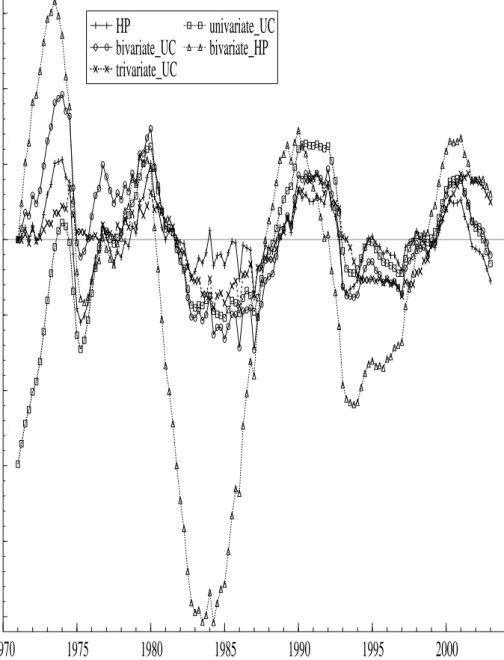
To give an indication of what the final output gap estimates (using the AWM data) look like, Figure 1 presents them for two univariate and three multivariate unobserved components (UC) estimators.17 These estimators are representative of those used both by
policy-makers and in related studies.18 For a review of these estimators and the
specifi-cations used see Appendix B. Although the five different estimates share the same shape, picking up the trough in the mid 1980s and the peak of the early 1990s, Figure 1 reminds us that inference is sensitive to measurement.19 The bivariate HP estimator produces
cycles with a far greater, indeed implausible, amplitude than the other estimators; this perhaps illustrates the dangers of imposing, rather than estimating, model parameters.
16We ignore the fact that GDP data are published with, at least, a one quarter lag.
17It is considered important to consider forecasts from more than one model given that model
uncer-tainty is an additional source of unceruncer-tainty associated with real-time estimates of the output gap. In fact, model uncertainty, in addition to parameter and data uncertainty, are the three sources of uncertainty affecting output gap estimates distinguished by the ECB in its October 2000 bulletin.
18We did also experiment with structural VAR based estimators of the output gap; see Mitchell (2003).
Results are not presented since they were not dissimilar to those presented in Table 1 for the bivariate and trivariate UC estimators. In any case, the methodological differences between VAR and UC estimators are, to a degree, illusionary since the VAR model can be re-written in state-space form; e.g. see DeSerres & Guay (1995). We should note, however, that when using the well known Blanchard-Quah identification method for VAR models, results were found to be extremely sensitive to the chosen lag order,p. Only with very highpdid we obtaina prioriplausible looking cycles; in this case the performance of the VAR cycle in real-time was similar to that of the multivariate UC estimators in Table 1. But whenp= 1 the correlation coefficient in Table 1 increased to 0.9. Although similar results, suggesting that reliable output gap estimates can be obtained in real-time for the Euro area, have been obtained by Camba-Mendez & Rodriguez-Palenzuela (2003), see their Figure 3, we believe this result is misleading. It is based on an implausible looking business cycle with, for example, an amplitude in the range -0.5% to 0.5%, rather than around -2.5% to 2.5% as is plausible and indeed typical for the other estimators.
19Other studies of the Eurozone business cycle, such as Runstler (2002) and Artis et al. (2004), find
We can also see the end-of-sample problem; the different estimators in Figure 1 do not agree about the current position of the cycle.
The real-time unreliability of output gap point estimates then is summarised in Ta-ble 1 for the five representative output gap estimators. Reflecting the fact that the five estimators in Table 1 can be interpreted within an UC framework [see Appendix B] and that UC models use the data in two ways, as well as considering the real-time estimate, Table 1 also examines the filtered estimates (or the quasi-final estimates in the parlance of Orphanides & van Norden (2002)).20 Let us denote the real-time estimates, based on
recursively updated estimates of the parameters of a given UC model Θ, by yC t|t; let y
C t|T
denote the final estimates of the output gap at time t, that use full-sample information
T to estimate Θ, and then let yC
t|t(ΘbT) denote the filtered estimates of the output gap at
time t using these full-sample based parameter estimates. For the univariate HP filter, as the only parameter is chosen a priori, clearly there is no parameter uncertainty; the filtered and real-time estimates are then equivalent; yC
t|t = y C
t|t(ΘbT).21 The reliability of
the real-time and filtered point estimates is summarised by their correlation against the final estimates and the noise-to-signal ratio (NSR). The NSR is the ratio of the RMSE of the revision (the difference between the real-time or filtered estimate and the final es-timate) to the standard deviation of the final estimate of the output gap.22 To provide
some indication of how sensitive results are to the chosen sample period, Table 1 con-trasts the performance of the real-time and filtered estimates computed over the period 1981q1-2000q1, with those computed over the period 1993q3-2000q1. This latter period was chosen as it is after both the peak in economic activity and the exchange-rate crises in the early 1990s. The final column of Table 1 provides a tentative indication of the impact of data revisions on real-time output gap estimation and presents the correlation of the real-time estimates, using real-time data vintages, against the final estimates using the final data vintage.23
Table 1 indicates that as the future becomes the present output gap estimates are
20UC models use the data in two ways in the sense that first they estimate the parameters of the model,
denoted by the vector Θ, and secondly they use these estimates to obtain the filtered and smoothed estimates of the output gap, namely the quasi-final and final estimates of the output gap, respectively. The filtered and smoothed estimates are the expected value of the output gap conditional on information available at timet(t= 1,2, ..., T) andT, whereT ≥t, respectively.
21In general, as the parameters of the UC model are estimated by maximum likelihood (ML) and
since ML estimation, under standard regularity conditions, delivers consistent estimators asymptotically (Θbt
p
→Θ,∀t) we should not expect a difference between real-time and filtered estimates. This holds as long as we view the UC model under consideration as the ‘true’ data-generating-process. In practice over time, in the presence of deterministic and stochastic nonstationarities, we should expect macroeconomists to revise the UC model they use to estimate the output gap.
22It is of theoretical interest that for correctly specified UC models this ratio in the case of the filtered
estimates (i.e. if we ignore the fact that we recursively re-estimate the parameters of the UC model) depends on the type of UC model considered; see Proietti (2004).
23It should be noted that the filtered estimates using the real-time data set (not reported in Table 1)
are not identical, as they should be, to those using the AWM data. They are, however, qualitatively similar. Due to its method of construction, detailed in Appendix A.1, the final column of the real-time data matrix for GDP is not identical to the AWM database.
revised. Real-time point estimates of the output gap in the Euro area, as in the US, are unreliable, in the sense that there is a large and important revision error. This is reflected by the correlation coefficients, over the period 1981q1-2000q1, being in the range 0.27-0.76 and the noise-to-signal ratio exceeding unity for three of the five output gap estimators, and for the remaining estimators being greater than 0.8. Reflecting the importance of
ex post information in re-defining the parameter values the filtered estimates are more reliable than the real-time estimates: correlation is higher and NSR lower. Parameter uncertainty appears to be a dominant source of the unreliability of real-time estimates. Interestingly, as in the US, data revisions do not appear to be a major source of revisions. The real-time estimates using real-time data were found to have similar properties to the real-time estimates that use final (AWM) data. This is reflected here in the final column of Table 1 that indicates that use of the real-time data, rather than the final data considered in the sixth column, leads to estimates correlated similarly with the final estimates.
There is some variation across estimators and the sample period. Comparing the estimators across the period 1981q1-2000q1, correlation ranges from 0.27 for the univariate HP measure to around 0.6-0.7 for the multivariate measures. In this sense it is encouraging that the move from univariate to multivariate measures of the output gap does lead to real time estimates better correlated with the final estimates. Adding ‘economic information’ appears to help. However, the multivariate estimators have higher noise-to-signal ratios than the univariate UC estimator.
This unreliability of real-time point estimates also shows up over the period 1993q3-2000q1. Although the univariate estimators are more reliable over this later period than 1981q1-2000q1, some of the multivariate estimators appear to be less reliable. This may reflect the fact that they do well at picking up the big movements, such as the cyclical peak in the early 1990s, but are worse at picking up the less volatile movements that appear to characterise the modern business cycle.
Table 1: The unreliability of real-time output gap point estimates. The correlation (cor) of alternative real-time and filtered estimates of the Eurozone output gap against the final estimates and the noise-to-signal ratio (N SR)
AWM data real-time data 1981q1-2000q1 1993q3-2000q1 1993q3-2000q1 real-time filtered real-time filtered real-time cor NSR cor NSR cor NSR cor NSR cor Uni HP 0.273 1.43 0.273 1.43 0.875 1.17 0.875 1.17 0.896 Uni UC 0.600 0.82 0.838 0.64 0.904 0.57 0.898 0.71 0.863 Bi UC 0.599 0.87 0.941 0.56 0.864 0.70 0.923 0.58 0.894 Bi HP 0.688 3.31 0.727 1.35 0.585 3.81 0.599 1.87 0.579 Tri UC 0.760 1.79 0.921 0.57 0.352 2.15 0.795 1.07 0.309
The findings of Table 1 beg the question, should we be surprised by this unreliability? To address this question, we therefore first take up the challenge of providing, in real-time, measures of uncertainty associated with real-time (point) estimates of the output gap,
via density forecasts. Secondly we evaluate them to ascertain whether the unreliability of output gap point estimates is surprising.24 Could we have anticipated this revision
error? In real-time was the revision error to the real-time estimate within the bounds of what we could have predicted? It is important to evaluate whether these measures of uncertainty offer a reliable indication of the degree of unreliability associated with output gap estimates as otherwise all that can be said is the bands are wider for, say, output gap estimate A than estimate B. Nothing can be inferred about the appropriateness of the bands per se.
3
Uncertainty associated with output gap estimates:
density estimates of the output gap
To capture fully the uncertainty associated with the real-time estimates, or forecasts, of the output gap, we construct density forecasts.25 Density forecasts of the output
gap provide an estimate of the probability distribution of its possible future values. In contrast, so-called “interval” and “event” forecasts provide specific information on forecast uncertainty that can be derived from the density forecast; interval forecasts specify the probability that the actual outcome will fall within a given interval while event forecasts focus on the probabilities of certain events, such as the probability of recession.
Questions then arise over how the density forecasts should be constructed. We consider a simple approach that relies on a state-space representation for the output gap estimator. In Section 3.1.1 we draw out some characteristics of this approach by noting that it can be seen to minimise forecast errors, in the sense that it is based on optimal forecasts.
3.1
Measuring the uncertainty associated with the output gap
Conditional on Gaussianity (of the disturbances driving the components of the state vector) and knowledge of the covariance matrix of the estimated state vector confidence intervals around the output gap can be presented, and density estimates derived.26 Before continuing our discussion we note that other distributions could be considered, although we confine attention in the rest of this paper to the Gaussian case since this both has the advantage of simplicity/familiarity and is sufficient to illustrate the role of density
24Although Orphanides & van Norden (2002), (pp. 578-582), provide measures of uncertainty associated
with their final (smoothed) and quasi-final (filtered) estimates they do not present, or evaluate, them for real-time estimates.
25For a review of density forecasting see Tay & Wallis (2000).
26The Kalman filter recursions automatically return estimates of the covariance matrix of the state
vector; see Harvey (1989). The diagonal elements of these matrices then can be used to construct the confidence intervals and density estimates. This approach has also been followed, for example, by Orphanides & van Norden (2002).
forecasting.27 For example, since 1996q1 the Bank of England has published the so-called “fan” chart of inflation in the UK, that allows for skewness. The fan chart is based analytically on the two-piece normal distribution; see Wallis (2004). This distribution has the convenient property that it can capture any asymmetries between upside and downside risk but still be computed using standard normal tables. Alternatively, rather than making some distributional assumption one could let the data decide; one could analyse the historical forecast errors. Past forecast errors are commonly used as a practical way of forecasting future errors; e.g. see Wallis (1989), pp. 55-56. Given the backward looking and mechanistic nature to this method of determining the distribution and its moments, it is important what historical sample period is chosen to analyse the errors. Historical errors are expected to provide a poor guide to future behaviour in the presence, for example, of regime changes.28
Continuing our discussion, let Pt|t denote the Kalman filter based variance of the
output gap at timet,yC
t|t, using information available up to timet; the output gap is one
of the elements of the state vector in the UC model. Then conditional on Gaussianity, the density is N(ytC|t, Pt|t). Denote the revision between the real-time and final estimates,
the focus of this paper, by Rt|T =yCt|T −y C
t|t. It is helpful to recall that with known and
constant parameters (i.e. for the filtered rather than real-time estimates of Table 1), this variancePt|t0 decreases ast0 increases; Pt|t=Pt|T+V ar(R∗
t|T). The variance of the filtered
(or one-sided) estimate is greater than that of the smoothed (or two-sided) estimate,
Pt|T, by a positive scalar equal to the variance of the revisions between the filtered and
smoothed estimatesR∗t|T where R∗t|T =yC
t|T −yCt|t(ΘbT). This is the familiar result that the
variance of the filtered (forecasted) estimate is equal to the variance of the outturn, Pt|T,
plus the square of the bias, V ar(R∗t|T). This assumes the revision process has mean zero so that V ar(R∗t|T) =E(R∗t|T)2.
Below in Section 3.2 we examine how to evaluate these interval and density forecasts once the final output gap estimate, yC
t|T whereT → ∞, has become available. 29
27The non-Gaussian case may require modification of the traditional state-space architecture. Durbin
& Koopman (2001) provide an account of how non-Gaussian (and nonlinear) state-space models can be handled using simulation techniques.
28Blake (1996) considered how stochastic simulation, with a coherent policy structure, can be used
as an alternative to historical errors to measure the uncertainty associated with, in his application, the inflation rate. It is explained that this is expected to deliver a better measure of uncertainty if a new policy regime (say a new target for inflation or EMU) has been adopted.
29These measures of uncertainty do not capture parameter uncertainty. Recall that for UC estimators
two measures of uncertainty associated with the cyclical component of output can be distinguished: filter and parameter uncertainty. If Θ were known Pt|t and Pt|T would indicate the uncertainty in the
Kalman-filter recursions. We call this uncertainty, filter uncertainty. However, there is an additional source of uncertainty if Θ is estimated, say by Θbt; i.e. Pt|t(Θbt) > Pt|t(Θ) and Pt|T(Θbt) > Pt|T(Θ).
Similarly to Orphanides & van Norden (2002) we did experiment with using analytical approximations (see Quenneville & Singh (2000)) to capture the parameter uncertainty. We should expect this to add to uncertainty most for those measures of the output gap that estimate most parameters, namely the multivariate measures. However, results were qualitatively similar to those presented here. In fact, as we will shall see in Figure 2, in general, filter uncertainty alone appears to often over-estimate the degree of
3.1.1 Understanding revisions to real-time output gap point estimates
In the absence of data revisions, revisions to real-time output gap estimates are explained by forecasting errors. This is seen as follows. Consider the final estimate of the output gap to be a known weighted linear function, that is say centered and symmetric, of the underlying GDP data, say yt:
ytC|T =B(L, F)yt, (1) where B(L, F) = b0+ ∞ X j=1 bj(Lj+Fj) and Lyt=yt−1 and F yt=yt+1.
Assuming the output gap is a weighted linear function of yt as in (1) involves no loss
in generality. De-trending filters, whether interpreted as parametric or nonparametric, can be seen to involve application of a moving-average filter to the raw data.30 Most
de-trending filters, such as the HP filter, imply a smooth two-sided moving average in the middle of the sample with no time-series observation receiving a large weight relative to its close neighbours. However, at the end of the sample the moving average becomes one-sided. It is well known that application of a one-sided filter will lead to more volatile estimates at the end of the sample as the weight on the last observation will be much higher than any of the weights associated with application of the filter in the middle of the sample since at the end of the sample the filter is unable to distinguish temporary from permanent shocks; e.g. see St-Amant & van Norden (1997).
The final estimate of the output gap is then given by:
ytC|T =B(L, F)yt=b0+ ∞ X j=1 bjyt−j + ∞ X j=1 bjyt+j. (2)
But in real-time the future values ofyt, namelyyt+1, yt+2...are unknown. To apply the
two-sided filter future values need to be forecasted. Denote the forecasts of yt+1, yt+2...
made at time t by E(yt+j|Ωt). Then we may define the real-time estimate as:
yCt|t=b0+ ∞ X j=1 bjyt−j+ ∞ X j=1 bjE(yt+j|Ωt). (3)
Subtracting (3) from (2) the revision is obtained as a function of the forecasting error, (yt+j−E(yt+j|Ωt)), yCt|T −y C t|t=Rt|T = ∞ X j=1 bj(yt+j−E(yt+j|Ωt)). (4) uncertainty and lead to excessively wide confidence bands.
30Traditionally business cycle analysts have often distinguished between parametric and nonparametric
de-trending methods. However, in reality this distinction is somewhat blurred. Many nonparametic filters, such as the Hodrick-Prescott and band-pass filters, can be rationalised as parametric; see Harvey & Jaeger (1993) and Harvey & Trimbur (2003). Furthermore, the parametric methods, like the nonparametric ones, are also ‘simply’ taking weighted averages of the data. For example, Harvey & Koopman (2000) and Koopman & Harvey (2003) present algorithms for deriving the moving-average weights for parametric (UC) models.
It follows that if these forecast errors are reduced the revision will decrease. Forecasting future values prior to de-trending facilitates use of a less one-sided de-trending filter.31
Crucially the density N(yC
t|t, Pt|t), considered above, can be seen implicitly to forecast
future values optimally. This follows from the fact that for a correctly specified model, application of the one-sided Kalman filter is equivalent to application of the two-sided filter (smoother) toytextended infinitely into the future with optimal forecasts. These optimal,
minimum mean square error [MSE], forecasts are derivedvia the Kalman filter, exploiting the state-space representation for a given output gap estimator. There is therefore no need for forecast extensions.
Only when the UC model is misspecified can forecast extensions, using an alternative forecasting model, help to attenuate revisions [lessen estimation MSE]. The importance of real-time testing for model misspecification is therefore apparent; see Harvey & Koopman (1992) for appropriate diagnostic tests for UC models. Of course, it is well known that good in-sample fit need not translate into good out-of-sample performance. For complete-ness and as a reference we do note here how forecast extensions might be used to derive an alternative density to N(yCt|t, Pt|t). See Mitchell (2003) for further discussion and an
empirical application.
Draw a large number R of realisations from the predictive density of future obser-vations ft+l = yt+l|y1, ..., yt (l = 1, ...h), based on an assumed forecasting model, say a
simple autoregressive (AR) or some other robust forecasting model.32 Then apply the
Kalman smoother to the series (y1, ..., yt) extended by the R forecasts to get R point
es-timates ybCt|t+h = E[yt|y1, ..., yt, ft+1, ..., ft+h]. The variance of these explicitly quantifies
the degree of uncertainty associated with the fact that future values of the (log) level of output are unknown but known to affect real-time estimates. However, the variance of this Monte-Carlo density must have less dispersion than that ofN(yC
t|t, Pt|t).
33This follows
from the ‘law of conditional variances’ that states that Pt|t can be decomposed into two
components, only the second of which is the variance V ar[bytC|t+h]:34
Pt|t=V ar(yb C
t |y1, ..., yt) =E[V ar[yt |y1, ..., yt, ft+1, ..., ft+h]] +V ar[yb C
t|t+h]. (5)
The first component E[V ar[yt |y1, ..., yt, ft+1, ..., ft+h]] is the average across R of the
variance Pt|t+h, delivered by the Kalman smoother.
Forecast extensions are not commonly used by analysts when using UC models to estimate the output gap. However, they have been employed when using nonparametric filters in real-time, whether for output gap estimation or seasonal extraction; e.g. see Wal-lis (1982), Stock & Watson (1999) and the discussion in van Norden (2004). Motivation
31In fact, as the forecasts are often a linear combination of the observed data, the filter applied is still
one-sided in the original data.
32It is well known that simple AR models can guard against unforeseen events such as structural breaks;
see Clements & Hendry (1999). See Garratt et al. (2003) for a discussion in terms of VAR models of how simulation techniques can be used to calculate density forecasts.
33Thanks to a referee for explaining this point. 34This ‘law’ states that for the random variablesy
rests on the fact that the “optimal” real-time or one-sided nonparametric filter, in the sense of delivering the minimum mean square revision error, involves application of the two-sided filter to the actual data extended by optimal linear forecasts; for a discussion in the context of seasonal adjustment see Wallis (1982).35
3.2
Evaluation of density forecasts of the output gap
While there exist well established techniques for theex post evaluation of point forecasts, often based around the RMSE of the forecast relative to the subsequent outturn, only re-cently has theex post evaluation of density forecasts attracted much attention. Currently, following Diebold et al. (1998), the most widespread approach is to evaluate density fore-casts statistically using the probability integral transform, itself a well-established result.36 Diebold et al. popularised the idea of evaluating a sample of density forecasts based on the idea that a density forecast can be considered “optimal” if the model for the density is correctly specified. One can then evaluate forecasts without the need to specify a loss function. This is attractive as it is often hard to define an appropriate general (economic) loss function.
We follow this approach and propose to evaluate real-time density forecasts of the output gap ex post with respect to the final estimates for the output gap yC
t|T, where
T → ∞.37 By treating these final estimates of the output gap as the ‘outturn’, evaluation
of real-time output gap density forecasts is analogous to evaluation of a sequence of rolling one-step ahead density forecasts, the case commonly considered in this recent density forecast evaluation literature.38
35See also van Norden (2004) who, when discussing nonparametric filters, neatly shows that extending
the series {yt} with optimal forecasts prior to de-trending can be seen as equivalent to deriving the
optimal one-sided filter, in terms of minimising E XT−1 j=0 bbjyT−j− X∞ j=−∞bjyT−j 2 with respect to bbj, wherebj are the optimal “ideal” weights given asbj= sinjuπj−sinjl for|j| ≥1 andbj =uπ−l forj = 0,
where uand l are the bands outside of which the spectral gain is zero, and inside of which the gain is unity.
36This methodology seeks to obtain the most “accurate” density forecast, in a statistical sense. It
can be contrasted with economic approaches to evaluating forecasts that evaluate forecasts in terms of their implied economic value, which derives from postulating a specific (economic) loss function; e.g. see Granger & Pesaran (2000) and Clements (2004). Other work has evaluated density forecasts using scoring rules; e.g. see Giacomini (2002). Alternatively, density forecasts can be evaluated by reducing them to an interval forecast. For example, Mitchell (2003) focused on the central 50% or inter-quartile-range forecast and the 95% confidence intervals implied by the density forecast. Christoffersen (1998) and Wallis (2003) have proposed likelihood-ratio and, asymptotically equivalent, Pearson chi-squared tests for the evaluation of such interval forecasts.
37Of course since the final estimates are themselves estimated, and not known with certainty, we could
consider evaluation of the real-time estimates not just against the final (point) estimate, as is traditional, but against the density of the final estimates. Mitchell (2003) did carry out such an exercise. However, it is perhaps little cause for celebration for policy-makers when analysts can only provide them with reliable interval and density forecasts of the output gap when the target (the final output gap they are trying to forecast) is itself acknowledged to be uncertain.
Irre-Real-time output gap density estimates are optimal, i.e. able to capture all aspects of the distribution ofyC
t|T, only when the sequence of probability integral transforms (pit’s),
zt, defined below, is independently and identically distributed (i.i.d.) with a uniform
distribution, U(0,1):
zt =
Z yt|TC
−∞
pt(u)du, or specifically in our case (6)
zt = Φ((ytC|T −y C t|t)/
p
Pt|t) , (7)
(t = 1,2, ...), where {pt(ytC|t)} are the sequence of estimated real-time density forecasts
and Φ is the standard normal cumulative density function (CDF); in our case pt(ytC|t) =
N(ytC|t, Pt|t).
By taking the inverse normal CDF transformation of {zt} to give, say, {zt∗} where
zt∗ = (yC t|T −y
C t|t)/
p
Pt|t are the standardised revision errors, a test for uniformity can
be considered equivalent to one for normality on {z∗t}; see Berkowitz (2001). This is useful as normality tests are widely seen to be more powerful than uniformity tests. However, testing is complicated by the fact that the impact of dependence on the tests for uniformity/normality is unknown, as is the impact of non-uniformity/normality on tests for dependence.
In the empirical application below we abstract from any perceived uncertainties re-garding the appropriateness of specific tests; we take an eclectic approach to testing i.i.d.
uniformity/normality. We consider a range of statistical tests that have been used in em-pirical studies.39 They have been used to detect misspecification in the mean, variance, spective of this, for a rolling sequence of optimal forecasts we should not expect serial dependence in the forecast errorsnyC
t|T −y C t|t
o
acrosst, yet alone in the standardised forecast errors{zt∗}, defined below. In contrast we should expect dependence when evaluating a sequence of rolling optimalh-step ahead point forecasts or optimal fixed-event point forecasts; e.g. see Clements & Hendry (1998), pp. 56-62. Recall that ytC|t are the real-time point estimates of the output gap considered in Table 1 (involving recursive re-estimation of the parameters of the UC model), not the filtered orquasi-final estimates. These use in-formation available at timeT, whereT > t, to estimate the parameters Θ of the UC model. We continue to denote these filtered estimatesyCt|t(ΘbT). Theoretically for a correctly specified UC model we should
expect dependence in the revisions between the filtered and smoothed estimatesnytC|T −ytC|t(ΘbT)
o . With fixed (constant and known) parameters, application of the Kalman smoother, used to derive the final estimates yC
t|T, will by construction induce serial dependence in these revisions across t. This is seen,
for example, by considering a simple UC model, say the random walk plus noise model. Fixed-point smoothing and fixed-interval smoothing will result in the revisions being serially correlated acrosst; e.g. see Harvey (1989) equation 3.6.15 (p.153) and equation 3.6.17 (p.154). The nature of this dependence is dictated by the nature of the process governing the determination ofyt; for further discussion see Proietti
(2004). As Proietti explains the smoother the trend the greater the revision. When no parameters are estimated, as with the HP filter, and the real-time and filtered estimates are equivalent in finite samples (as well as asymptotically which they are for all UC models) it should be no surprise (and in this sense constitute no violation of optimality) that revisions are serially correlated; it is a statistical artefact of the method chosen to identify the final estimates of the output gap.
39Alternatively, graphical means of exploratory data analysis are often used to examine the quality of
skewness and/or kurtosis of the forecasts. They differ not just in terms of their moti-vation, which we do not discuss here, but with respect to what they test. Some test for misspecification in all of the first four moments, while others focus on specific moments. Below we summarise relevant aspects of the tests:
1. Kolmogorov-Smirnov (KS) test for uniformity of{zt}. The KS test relies on random
sampling. As noted, for example, by Diebold et al. (1999) the effect of dependence on the distribution of the KS test statistic is unknown.
2. Anderson and Darling (AD) test for uniformity of {zt}. Using Monte-Carlo Noceti
et al. (2003) found the AD test to have more power to detect misspecification in the first four moments than the KS test (and related distributional tests).
3. The Bai and Ng (BN) ‘robust’ test of normality on {zt∗}; see Bai & Ng (2003). Bai and Ng extend traditional (Jarque-Bera) normality tests, designed for i.i.d.
data, to weakly dependent data. Essentially, any serial dependence is taken into account by consistently estimating the long-run variance (the spectral density at frequency zero) using a HAC estimator that is robust to serial dependence (and heteroscedasticity). This test looks at the coefficients of skewness and kurtosis and therefore has no power to detect misspecification in the first two moments.
4. A Ljung-Box (LB) test of independence of{zt}. To test for independence of the{zt}
series we use the Ljung-Box test for auto-correlation; see Harvey (1989), p. 259. Since dependence may occur in higher moments we consider (zt−z)
j
forj = 1,2,3; results are denoted LB1, LB2 and LB3, respectively.
5. The Hong joint test for uniformity and independence applied to {zt}; see Hong
(2002). This test is theoretically attractive as it offers a joint test. This means one can control the size of the test, something that cannot easily be done using separate tests for uniformity/normality and independence. Hong’s joint test for
i.i.d. U(0,1) is based on generalised spectral analysis. We estimate the spectrum nonparametrically using the Bartlett kernel and, following Hong, use a data-driven approach to determine the bandwidth. This requires us to choose a preliminary bandwidth. Hong proposes two test statistics, M0 and M1. Hong recommends
M1 in small samples; accordingly we consider this. Hong also proposes a test for independence robust to non-uniformity.
4
The uncertainty of real-time output gap estimates
in the Euro area: density forecasts
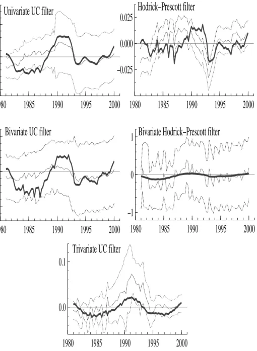
Figure 2 provides a visual indication of the degree of estimated real-time uncertainty for the five UC based estimators of the output gap by plotting 95% confidence intervals around the point estimates. There are striking differences in the degree of uncertainty
(predicted in real-time) associated with the real-time estimates across the alternative estimators of the output gap. As is to be expected, uncertainty is lowest for the Hodrick-Prescott estimator. It is largest for the bivariate Hodrick-Hodrick-Prescott estimator where the degree of uncertainty is, incredibly, large.40 This reflects the imposition of a priori para-metric restrictions leading to a poorly defined model, in a statistical sense, where there is considerable uncertainty about the values of the remaining free parameters.
The Gaussian bands are very rarely significantly different from zero; policy-makers on this basis could never be sure about the position of the business cycle. With estimates of the standard error often in excess of 1%, point estimates for the output gap must be at least ±2% to be statistically significant, at traditional significance levels. But is the finding that these bands nearly always cover zero, in fact, correctly quantifying the degree of uncertainty associated with real-time estimates? This can be analysed formally using the statistical tests outlined in Section 3.2. First, however, it is useful simply to contrast the confidence bands for each measure with the actual outturn (printed in bold face) by looking again at Figure 2. There are again important differences across the alternative output gap estimators. The outturn frequently falls outside the 95% confidence bands for the Hodrick-Prescott estimator.
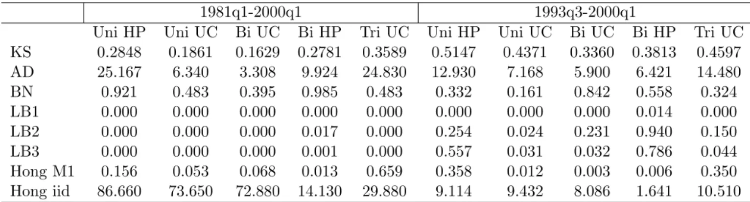
Table 2 complements Figure 2 by providing the results of the formal evaluation tests for the predicted measures of uncertainty. Density evaluation tests are performed both over the periods 1981q1-2000q1 and 1993q3-2000q1. Perhaps not unsurprisingly given the evidence in Figure 2, the consensus across these tests is that the computed measures of uncertainty do not provide a statistically satisfactory indication of the degree of uncer-tainty associated with real-time output gap estimates when evaluated against the point estimate for the outturn.
The most apparent reason for failure of the density forecasts from Table 2 is serial de-pendence in the first moment of{zt}, although there is some evidence that this dependence
is less acute over the 1993q3-2000q1 period.41 This shows up in both the Ljung-Box and
robust tests for i.i.d.(Hong iid). This serial dependence is consistent with our finding of considerable persistence in the (scaled) revisions. It is accordant with the view that even if the model used to estimate the output gap is well-specified in-sample, out-of-sample
40The narrow bands for the univariate HP estimator, and the implausible estimates for the bivariate
HP estimator, may also be explained by misspecification of the UC model underlying the HP filter. This misspecification, as discussed above, will deliver sub-optimal inference. Empirically we did find support for this view; we subjected the estimated models to a range of misspecification tests as suggested by Harvey & Koopman (1992). The HP models, univariate and bivariate, appeared to suffer from excessive residual correlation suggesting that the models fail to pick up the dynamics adequately. However, we continue to consider both models as they provide useful benchmarks.
41We also considered the interval evaluation tests referred to above. Like the density evaluation tests
they comprise both distributional and dependence aspects. They require a ‘good’ interval forecast to both have correct (unconditional) coverage, i.e. a ‘hit rate’ equal to the nominal rate, and for these hits and misses to exhibit no temporal pattern (independence). These tests did not reject the 95% and central 50% interval forecasts for the trivariate UC model. There is also some support for the bivariate UC interval forecasts; see Mitchell (2003). The density evaluation results suggest, however, that not all possible interval forecasts, and there are an infinite number of them, will offer a reliable indication of the degree of uncertainty.
Table 2: Evaluation of real-time output gap density estimates
1981q1-2000q1 1993q3-2000q1
Uni HP Uni UC Bi UC Bi HP Tri UC Uni HP Uni UC Bi UC Bi HP Tri UC KS 0.2848 0.1861 0.1629 0.2781 0.3589 0.5147 0.4371 0.3360 0.3813 0.4597 AD 25.167 6.340 3.308 9.924 24.830 12.930 7.168 5.900 6.421 14.480 BN 0.921 0.483 0.395 0.985 0.483 0.332 0.161 0.842 0.558 0.324 LB1 0.000 0.000 0.000 0.000 0.000 0.000 0.000 0.000 0.014 0.000 LB2 0.000 0.000 0.000 0.017 0.000 0.254 0.024 0.231 0.940 0.150 LB3 0.000 0.000 0.000 0.001 0.000 0.557 0.031 0.032 0.786 0.044 Hong M1 0.156 0.053 0.068 0.013 0.659 0.358 0.012 0.003 0.006 0.350 Hong iid 86.660 73.650 72.880 14.130 29.880 9.114 9.432 8.086 1.641 10.510 Notes: KS is the Kolmogorov-Smirnov statistic with associated 95% critical value 0.25; AD is the
Anderson-Darling statistic which has an associated 95% critical value of 2.502; BN is the p-value of the Bai-Ng robust test for normality; LB1, LB2 and LB3 are the p-values for the Ljung-Box tests for serial correlation in the first, second and third power; Hong M1 is the Hong joint test statistic for uniformity and independence with associated 95% critical value of 0.052; Hong iid is the Hong test statistic for independence that is robust to non-uniformity with associated 95% critical value of 1.96
(unforeseen) structural shocks lead one to revise the model (in particular the parameter estimates) used to identify and estimate the cycle resulting in serially correlated revisions to real-time estimates.42 Although it is difficult to disentangle the joint test fori.i.d.
uni-formity/normality, there does appear to be some support for the assumed distribution. Although the KS and AD tests are largely unsupportive, the distributional test of Bai and Ng, that in contrast to these tests is designed to be robust to the dependence, provides support with p-values greater than 0.15 in all cases.
Therefore it appears that not just, as indicated in Table 1, are real-time point estimates of the output gap unreliable but so are measures of uncertainty associated with them. Alternative measures of uncertainty, of course, may do better than the one considered here. Future work should consider other ways of measuring the uncertainty associated with real-time estimates with the aim of finding the ‘correct’ density estimate. Re-calibrating or bias correcting the density forecasts is one option.
5
Implications of output gap uncertainty
This section draws out some implications of our empirical finding that not just are real-time output gap point estimates unreliable but so are their associated measures of un-certainty. We focus on the effect of this uncertainty on prescriptions from policy rules.
42As noted above if we believe the UC model underlying the HP filter is correctly specified (which as
indicated we do not) we should expect the revisions associated with these optimal real-time HP estimates to be serially correlated since the real-time estimates equal the filtered estimates.
Alternatively, given the much debated importance of the output gap in forecasting infla-tion, we could consider the effect on forecasts of inflation. Analogously to the discussion below we should expect real-time uncertainty about the output gap to translate into (even greater) uncertainty about future values of inflation, in other words a widerfan-chart.
5.1
Taylor-type rules
Taylor-type rules model the interest rate as a function of both the deviation of inflation from its target level and the output gap. They have been found both to match the historical behaviour of interest rates in many countries and to perform well (in the sense of minimising some type of loss function over output, inflation and interest rate variations) relative to optimal feedback rules in simulation exercises; e.g. see Clarida et al. (1998) and Peersman & Smets (1999), respectively.43 Recently Taylor rules have also been discussed
with reference to the ECB; e.g. see Peersman & Smets (1999) and Gerlach & Schnabel (2000). They could be a useful informal benchmark to analyse and predict how the ECB sets interest rates. We address this issue in this section focusing on how the considerable uncertainty that appears to exist about real-time output gap estimates translates into uncertainty about monetary policy. This uncertainty is again best represented by a density forecast.
The principle of certainty equivalence might lead us to expect that uncertainty about real-time output gap estimates should have no effect on the optimal response to them in monetary policy rules.44 However, we know from empirical applications to the US
that the difference between real-time and final estimates is not irrelevant when analysing and using monetary policy rules; see Orphanides (2001, 2003b). At a theoretical level, uncertainty will also impact on the optimal coefficients in Taylor-rules. Uncertainty is expected to attenuate the coefficient on the real-time output gap estimate.45 As long as
we view the problem in real-time as one of extracting from the real-time data a signal (our best guess of the ‘final’ value of the output gap) this holds even when we consider optimal, as well as restricted or simple, policy rules; see Swanson (2004).
Signal extraction implies that the real-time estimate is additively composed of the final estimate, the signal yC
t|T, plus a noise component representing measurement error;
i.e. yC
t|t = ytC|T +ηt, where ηt is distributed independently of yCt|T. While in a
linear-quadratic model, optimal policy is certainty equivalent with respect to the best guess
E(yC
t|T), that is optimal policy reacts to E(y C t|T) equivalently to y C t|T treating E(y C t|T) as
43In establishing that Taylor-type rules often provide a good characterisation of interest rate behaviour
focus has been on the point estimates from the Taylor rule. As we stress in this paper it is better to view these estimates as central points of ranges of uncertainty.
44This principle states that in the linear-quadratic case (quadratic loss function and linear constraints)
the optimal decision rule is independent of the problem’s noise statistics. In other words, policy-makers can ignore uncertainties about the shocks that hit the economy and set policy as if they were certain. For a textbook discussion and proof see Ljungqvist & Sargent (2000), pp. 57-59. For explicit discussion with respect to optimal monetary policy rules see, for example, Swanson (2004).
45See, for example, Aoki (2003), Ehrmann & Smets (2003), Orphanides (2003a), Rudebusch (2001)
if certain, it is not certainty equivalent with respect to the actual observed real-time output gap estimates yC
t|t. This is because y C
t|t 6=E(y C
t|T); via the Wiener-Kolmogorov (or
equivalently Kalman) filter E(yC
t|T) = ay C t|t where a = ACF(yC t|T) ACF(yC t|t)
, where ACF denotes the autocovariance generating function.46 Only when we consider the “news”, rather than “noise”, model: yC
t|T = y C
t|t+ηt where ηt is mean zero and distributed independently of
yCt|t, does E(ytC|T) =yCt|t and certainty equivalence hold.47
In the noise model it is optimal for policy-makers to attenuate their response to vari-ables about which uncertainty has increased; see Swanson (2004). This attenuation has been found to bring the optimal coefficients into line with historical (empirical) estimates. In the absence of uncertainty the optimal coefficients are often larger; see Smets (1999) and Rudebusch (2001).
The empirical support in this paper for the view that, across widely used output gap estimators, real-time output gap point estimates are unreliable, specifically support for the noise model, implies that in real-time policy-makers do require reliable estimates of the uncertainty associated with these estimates. These estimates should dictate the strength of their optimal reaction to movements in real-time output gap data at a given point in time. Informally we know that central bankers do attach health warnings to data; they know data are imperfect and subject to revision. Only when policy-makers believe the output gap estimates they consult in real-time to be reliable (i.e. consistent with the news model) should they ignore the uncertainty associated with their estimates; the empirical evidence presented in this paper suggests that perhaps it would be unwise for the ECB
46WhenyC
t is a stationary Gaussian random variable then the ACF is defined as ACF(yCt) = γ0+
X∞ j=1γj(L j+Fj), whereCov(yC t , y C t−k) =γk fork= 0,±1,±2, ....
47It is clearly important to establish whether real-time output gap estimates are consistent with the
noise or news paradigm. Therefore, empirically we tested for news versus noisevia a series of Mincer-Zarnowitz tests; e.g. see Clements & Hendry (1998) pp. 56-59. These essentially test if revisions are unbiased (weakly rational) as well as efficient or (strongly) rational. The null hypothesis of news amounts to testing, via a Wald or F-test that is robust to serial correlation and heteroscedastictiy, the joint hypothesis thatb0= 0 andb1= 0 in the regression: Rt|T =b0+b1yCt|t+t.Under the noise model,ηtis
correlated withyCt|tand will therefore help predict the subsequent revision Rt|T, implying a rejection of
the null. Across the five output gap estimators we found no support for the news model (p-values equal to 0.000). The preliminary, or real-time, estimate can help predict the subsequent revision. This suggests that real time estimates are not rational expectations of the final estimates. This finding is also supported by the fact that the standard deviation of the real-time estimates is not always less than the standard deviation to the final estimates. For completeness we note that for a correctly specified UC model the filtered estimates yC
t|t(ΘbT) are rational expectations of the final estimates yCt|T. This follows from the
fact that yCt|t(ΘbT) is the minimum MSE estimator of the true (unknown) ytC. Given normality, these
conditional expectations are equivalent to orthogonal projections. Therefore, yC
t|t(ΘbT) is the orthogonal
projection ofyCt on Ωt.SimilarlyyCt|T is the orthogonal projection ofytC on ΩT. Via the law of iterated
expectations E(yC
t|T |Ωt) =E(E(yCt |ΩT)|Ωt) =E(yCt |Ωt) =yCt|t(ΘbT)⇒E(ytC|T −y C
t|t(ΘbT)|Ωt) = 0.
So, the filtered estimates can be also seen as the orthogonal projection of the final estimates on Ωt.This
implies both that the revisions (between the filtered and final estimates) are unbiased, and that this revision is orthogonal to the filtered estimate (rationality).
to believe this.
Figure 2 also suggests that these uncertainty estimates are heteroscedastic; V ar(ηt) =
σ2
ηt 6=σ2η. For the trivariate UC estimator, in particular, we observe an increase in
uncer-tainty as the economy approached the turning point of the early 1990s, and a decrease thereafter. However, the pertinent result to extract from the empirical analysis in Sec-tion 4 is that typical output estimators when applied to Euro area data do not provide policy-makers, in real-time, with reliable estimates of this uncertainty σ2ηt. More work along the lines of Rudebusch (2002), p. 424, is therefore required to establish using sim-ulated models the consequences of using unreliable estimates of the uncertainty estimate in real-time. Perhaps the unreliability in real-time of uncertainty, as well as point, output gap estimates will strengthen support for policy rules that ignore the output gap, such as nominal income rules; for further discussion see Rudebusch (2002). Alternatively given the apparent scale of the uncertainty associated with output gap estimates in real-time perhaps one should consider a nonlinear policy rule where policy-makers respond more aggressively as the uncertainty reduces; e.g. see Meyer et al. (2001). We find that typi-cally it takes about three years for output gap estimates to begin to settle down at their ‘final’ values.
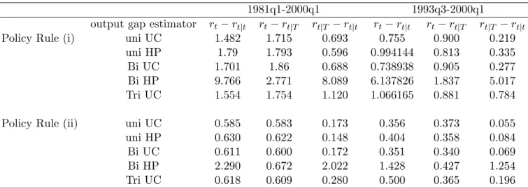
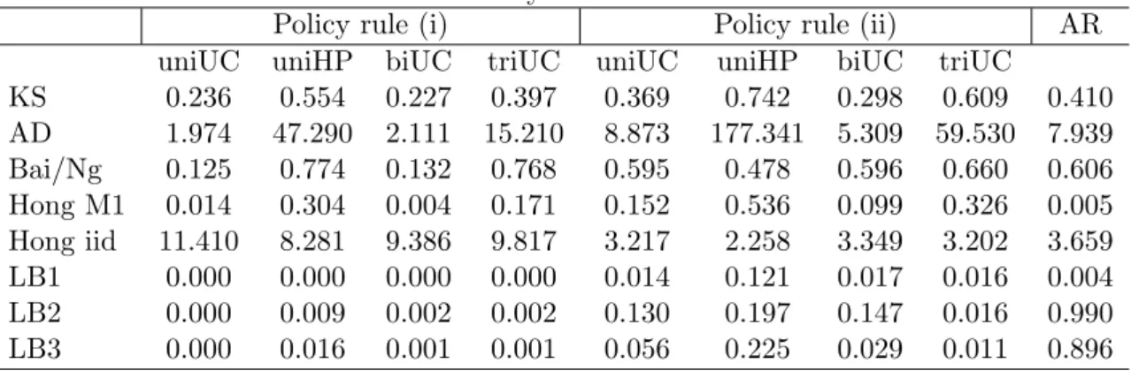
It is therefore important for policy-makers to look at the uncertainty of real-time out-put gap estimates. The remainder of this section draws out three practical implications of this uncertainty. First, we compare real-time policy recommendations with those based on final output gap data. Notwithstanding the limitations of having to base our analysis on AWM data, it is important to gain some indication of how well Taylor-type rules, using both final and real-time output gap data, explain the ECB’s notional behaviour. Existing work, comparing real-time and final data, has focused on the US; see Orphanides (2001, 2003b). Secondly, we illustrate how uncertainty about real-time output gap esti-mates translates into uncertainty about the value of the policy instrument. In accordance with our focus in this paper, we then evaluate whether the implied density forecasts for the interest rate offer a good characterisation of actual movements in the interest rate. Conceptually this represents an important departure from existing studies that test how well the Taylor rule fits the data with a focus on point estimates. Thirdly, we propose a simple means of potentially improving real-time density forecasts of