Closed Form Transient Solution of Continuous
Time Markov Chains Through Uniformization
Llorenc¸ Cerd`a-Alabern
Univ. Polit`ecnica de Catalunya, Computer Architecture Dep. Barcelona, Spain
Email: [email protected]
Abstract—This paper derives a mapping between a close form transient solution of a continuous time Markov chain (CTMC), and a close form transient solution of one of its uniformized discrete time Markov chains. This result is used to propose a new method to compute the transient solution of CTMCs. The method is simple to implement and has important benefits: (i) It yields a closed-form solution. (ii) It can be used to compute the transient solution for general CTMCs (even with absorbing states, or defective matrices). (iii) It can be used even for chains having a large number of states.
Index Terms—Markov chains, transient solution, Eigenvectors method, Vandermonde system, Uniformization.
I. INTRODUCTION
Probabilistic modeling using Markov chains has been suc-cessfully exploited in almost all fields of modern applied mathematics, and particularly in computer communications. Thestationarysolution of a Markov chain is easier to compute than the transient solution, and it is enough in many cases. However, some applications, as reliability modeling [1], mul-tiprocessor load balancing [2], network survivability [3] and others are primarily interested in the transient solution. Many methods have been proposed to compute the transient solution of Markov chains. Some examples are the approaches based on Laplace transform techniques [1], [4], the exponential ma-trix [5], finite-differencing [6], differential equation solvers [7], Markov fluid models [8], etc. The chapter 8 of the classic book of Stewart [9] is dedicated to this topic.
This paper focuses on the class of methods based on the undetermined coefficients approach. This approach consists on making an intelligent guess of a closed-form expression with constant coefficients for the solution of an equation, and solve for these coefficients using boundary conditions. The undetermined coefficients approach has been successfully used to find the solution of many difference and differential equations (see e.g. [10]). The transient solution of a Discrete or Continuous Time Markov Chain (DTMC and CTMC), is the solution of a difference or differential equation respectively. Therefore, they are suited to be computed using algorithms based on the undetermined coefficients approach.
The well known Eigenvectors method [5], explained later in this paper, belongs to the class of undetermined coefficients approaches. Another possibility is applying the undetermined coefficients approach directly to the solution of the Markov chain, expressed in terms of its eigenvalues, as done e.g.
in [11]. By doing so, the undetermined coefficients are ob-tained by solving a Vandermonde system of equations. For this reason thorough the paper this method will be referred to as the Vandermonde method. In this paper the pros and cons of these techniques are analyzed. Furthermore, we derive the mapping between the undetermined coefficients of a CTMC and those of one of its uniformized DTMCs. This result is of theoretical interest, and to the best of our knowledge, this is the first time that such mapping is established. We use this result to propose a novel approach to compute a close form transient solution of a CTMC. Thorough the paper, this novel proposal will be referred to as the Uniformized Vandermonde (UV) method. Numerical results show that it yields a simple yet powerful technique to compute a close form transient solution of a CTMC.
Before introducing the Uniformized Vandermonde method the paper dedicates sections II to V to review the solution of DTMC and CTMC using the undetermined coefficients approach. Most of the contents of these sections are not a con-tribution of this paper. For instance, the Eigenvectors method applied to Markov chains can be found in classic books as [12, sec. 4.8]. The expression for the exponential matrix having confluent eigenvalues (equation (14) in section IV) can be found in previous works [13], [14], [15], [7]. Nevertheless, to our best knowledge, the equivalent equation for a DTMC (equation (2), section II), has been not previously reported in the literature. The CTMC counterparts have been included for the sake of completeness, because they are the basis of Uniformized Vandermonde method presented in section VI, and because they are used in the numerical results presented in later sections. An additional reason is that, even if the Vandermonde method is one of the simplest ways to compute the transient solution of a Markov chain, it is not covered, or it is done superficially, in the books found in the literature. This paper tries to fill this gap, highlighting the striking parallelism that exists when this method is used to compute the transient solution of DTMCs and CTMCs.
The rest of the paper is organized as follows. First, the function with constant coefficients for the transient solution of a DTMC is presented in section II, and in section III the coefficients are computed using the Eigenvectors and Vandermonde methods. In sections IV and V, the same it is done for a CTMC. The Uniformized Vandermonde method is presented in section VI, in section VII numerical experiments
are carried out analyzing the different methods described in this paper. Section VIII discuss the stability of the Uniformized Vandermonde method. Finally, concluding remarks are given in Section IX.
II. DISCRETETIMEMARKOVCHAINS
Let X(n) be a homogeneous finite-state discrete-time Markov chain withkstates, and one step transition probability matrix of sizek,Pk×k. The transient solution is given by the
powers of P[12]:
π(n) =π(0)Pn, n≥0 (1)
where π(0) is the initial distribution, and the components of the row vectorπ(n)are the probabilities
πj(n) =P rob
X(n) =j π(0) , 1≤j ≤k, n≥0
If we are interested in computingπj(n)for only a reduced
number of states, the following expression may be more efficient that computing the powers of the matrix P.
Theorem 1 Let λl, l = 1,· · ·L be the eigenvalues of P, each with multiplicity kl (kl ≥ 1, Plkl = k). Without loss of generality, assume a possible eigenvalue λ1 = 0 with
multiplicity k1. Then: πj(n) = k1−1 X m=0 a(1j,m)δn−m+ L X l=2 λnl kl−1 X m=0 a(jl,m)nm, 1≤j≤k, n≥0 (2)
where a(jl,m) are constants that thorough the paper will be referred to as undetermined coefficients, and δk is the Kronecker’s delta (δk= 1 fork= 0and 0 otherwise).
The proof of equation (2) is skipped for the sake of space.
Remark 1 Assume that the Markov chain has the eigenvalue
λ2 = 1 with multiplicity k2 >1. Clearly, the polynomial in
equation (2) corresponding to this eigenvalue:
p(2)j (n) =
k2−1
X
m=0
a(2j ,m)nm (3)
must have the coefficients a(2j,m)= 0, form= 1,· · · , k2−1.
Otherwise, the equation (2) will be unbounded (the poly-nomial (3) would diverge when n → ∞). Therefore, the eigenvalueλ2= 1has only 1 undetermined coefficient (i.e. the
polynomial(3)corresponding toλ2= 1isp (2)
j (n) =a
(2,0)
j ). A consequence of this fact is that the geometric multiplicity of the eigenvalueλ2= 1must be equal to its multiplicity1,k2. There
may be other eigenvalues with geometric multiplicity larger than 1. However, it is not necessary to compute the geometric multiplicity of the eigenvalues: if the geometric multiplicity
1The geometric multiplicity is defined as the number of linearly independent eigenvectors associated with the eigenvalue. Thorough the paper we shall use the termconfluent to refer to eigenvalues having a multiplicity larger than their geometric multiplicity.
of an eigenvalue λl is gl, when solving for a
(l,m)
j it will be obtained thata(jl,m)= 0 form > kl−gl.
III. UNDETERMINEDCOEFFICIENTS OF ADTMC In equation (2) there are up tok undetermined coefficients a(jl,m) of πj(n)to be determined. This paper focuses on the
computation of these coefficients. Thorough the paper the sentence the UC of πj(n), or simply the UC, will be used
to refer to the undetermined coefficients a(jl,m) of πj(n).
Additionally, to denote the UC of πj(n) it will be used the
notation: u u uj= h u u u(1)j · · · uuu(jL)i T , (4)
where uuuj is a column vector with uuu
(l) j = h a(jl,0) · · · a(l,kl−1) j i
, l = 1,· · ·L (thorough the paper we shall use()Tas the transpose operator). In the following two
methods to compute the UC of πj(n)are described. A. Eigenvectors Method
If the matrix P is diagonalizable, the Jordan blocs are
reduced to scalars: Jl = λl, and the matrix P admits the
spectral decomposition: P = L−1Λ L, where Λ is the
diagonal matrix Λ = diag(λ1,· · ·λk), and L is a matrix
whose rows, l1,· · ·lk, are the left-hand eigenvectors of P.
Since Λn = diag(λn1,· · ·λnk), substituting into equation (1)
we have π(n) =π(0)Pn=π(0)L−1ΛnL= k X i=1 aiλni li (5) where we assumeλn
i =δn for anyλi = 0. Defining the row
vector a =
a1 · · · ak, the constantsai can be obtained
solving the system of equations:
a L=π(0) (6)
and, by (5), the UC ofπj(n)(the vectoruj) are given by the
element wise product of the vectorathat solves the system (6),
and thej column ofL.
If we want to use right eigenvectors, perhaps because our numerical tool only computes them, then we can proceed as follows. LetRbe a matrix whose columns,r1,· · ·rk, are the
right-hand eigenvectors of (P)T. Then, (P)T = R Λ R−1,
and: (π(n))T= k X i=1 biλni ri (7)
Defining the column vectorb=b1 · · · bk
T
, the constants bi can be obtained solving the system of equations:
R b= (π(0))T (8)
and, by (7), the vectoruuuj (see equation (4)) is given by the
element wise product of the vectorbthat solves the system (8),
and thej row ofR.
Note that Pis diagonalizable only if the geometric
matrix is said to be non-defective). This is an important restriction of this method.
B. Vandermonde Method
The UC of πj(n), 1≤j ≤k can be obtained solving the
system of equations that results from imposing the boundary conditions to equation (2):
πj(n) = (π(0)Pn)j (9)
where the notation(xxx)jrefers to thejcomponent of the vector
x x
x. Note that we need substituting in (9) forn= 0,1,· · ·, up to the number of UC to be determined minus 1. If we do not use the fact that the geometric multiplicity of some eigenvalues may be larger that 1, then there will be k UC, where k is the number of states of the Markov chain, i.e. the size of the square matrixP(see remark 1). For the sake of simplicity, in
the rest of the paper, if not otherwise stated, we shall obviate this fact and assume a Markov chain with kstates, andkUC to be determined. Using (2) and substituting in (9) we have that the vectoruuuj with the UC ofπj(n), defined by (4), can
be obtained solving the system of equations:
A1 · · · ALuuuj=B (10)
where the sub-matricesAk×kl
l ,l= 1,· · ·L, (λ1= 0,λl6= 0)
are given by:
Ak×k1 1 = 1 0 · · · 0 0 1 · · · 0 · · · Akl×kl = 1 0 · · · 0 λl λl · · · λl λ2 l 2λ 2 l · · · 2 kl−1λ2 l · · · λn l n λ n l · · · n kl−1λn l · · · (11)
Notice that the elements of (11) are given by: (Ak×kl l )ij = (i−1)j−1λil−1, 1 ≤ i ≤ k, 1 ≤ j ≤ kl. B is the column vector: B= πj(0) (π(0)P)j (π(0)P2)j· · · (π(0)Pk−1)j T (12) Note that if the chain starts in statei with probability 1 (i.e., π(0) is a probability vector with the probability 1 in the component i), then B = [δij (P)ij (P2)ij· · · (Pk−1)ij]T,
where δij is the Kronecker’s delta (δij = 1 for i=j, and 0
otherwise).
Using this approach, uuuj is obtained solving a confluent
Vandermonde system of equations, for which there exist abundant literature and fast numerical methods. One example is the method of Bj¨or and Pereyra [16]. However, for large matrices this method fails to give accurate results, due to rounding errors. Therefore, in the numerical experiments given in section VII it was found more convenient building the Vandermonde matrix and solving the system using a QR decomposition [17].
This approach has the advantage over the Eigenvectors
method that the matrix P can be defective. Therefore, this
approach gives a more general solution.
Remark 2 In order to compute the vector B it is not nec-essary the computation of the powers of the matrix P, as it may seem from equation(12). This would be costly for large matrices. Note that equation (12)can be implemented as the product of a row vector,r,k−1times the matrixP, as shown in the algorithm III.1. Note also that if we are interested in
πj(n)for j ={j1,· · ·jn}, then it is convenient to solve the system (10) for the matrix Bk×|j| that would be computed
using algorithm III.1 with the indexesj={j1,· · ·jn}. We use the notation|j|for the cardinality of the setj={j1,· · ·jn}. Algorithm III.1 Computation of matrixBk×|j|. We use the notationv[j]for a subvector of|j|elements ofv indexed by
the setj={j1,· · ·jn}.B[i,]denotes rowi of matrixB.
1: B[1,]←π0[j] 2: r←π0 3: for alliin2 :kdo 4: r←r P 5: B[i,]←r[j] 6: end for
IV. CONTINUOUSTIMEMARKOVCHAINS
Let X(t) be an homogeneous finite-state continuous-time Markov Chain withkstates, and infinitesimal generator (rate matrix) of size k, Qk×k. The transient solution is given by
the exponential matrix eQt [12]:
π(t) =π(0)eQt, t≥0 (13)
whereπ(0) is the initial distribution and the components of the row vectorπ(t)are the probabilities
πj(t) =P rob
X(t) =j π(0) , 1≤j≤k, t≥0
An expression forπj(t)can be obtained analogously to the
discrete time case.
Theorem 2 Letλl,l= 1,· · ·Lbe the eigenvalues ofQ, each with multiplicitykl (kl≥1,Plkl=k), then:
πj(t) = L X l=1 eλlt kl−1 X m=0 a(jl,m)tm, 1≤j≤k, t≥0 (14) Equation (14) has been previously used in the literature [13], [14], [15], [7], and it will not be proved here.
Remark 3 Note that, in contrast to the case of a DTMC (see theorem 1), now it is not necessary a special attention to the eigenvalueλl= 0. In fact, since eλlt= 1 forλl= 0, the UC associated withλl= 0in a CTMC is the only one that do not vanish in πj(t) whent → ∞. Thus,λl = 0 is for a CTMC equivalent to what the eigenvalueλl = 1is for a DTMC. In the rest of the paper we shall refer to the eigenvalue equal to1 of a stochastic matrix P, and 0 of a rate matrix Q, as the dominant eigenvalue. Additionally, the remark 1, regarding
to the eigenvalue λ1= 1in a DTMC, has its counterpart for
the eigenvalue λ1 = 0 in a CTMC: assume that the Markov
chain has the eigenvalue λ1 = 0 with multiplicity k1 > 1.
Clearly, the polynomial corresponding to this eigenvalue:
p(1)j (t) =
k1−1
X
m=0
a(1j ,m)tm (15)
must have the coefficients a(1j,m)= 0, form= 1,· · · , k1−1.
Otherwise, the equation (14)will be unbounded (the polyno-mial (15) would diverge when t → ∞). Therefore, for the dominant eigenvalue of both DTMC and CTMC there will be associated only 1 undetermined coefficient.
V. UNDETERMINEDCOEFFICIENTS OF ACTMC In equation (14) there are up tokUCsa(jl,m)ofπj(t)to be
determined. The two methods described in section III can be applied to obtain the UC of πj(t). The Eigenvectors method
described in section III-A is almost identical for a CTMC, thus, it will not be repeated here. The only difference is that λni in equations (5) and (7), are now eλit, and, in contrast
to the DTMC, it is not necessary a special attention to the eigenvalue λl = 0. Note that for CTMCs the Eigenvectors
method also requires the matrix matrixQto be non-defective.
This property only holds in some special cases, as in M/M/c queues. This fact has been exploited in [18] to obtain a close form transient solution for these class of queues.
A. Vandermonde Method
The UC of πj(t), 1 ≤j ≤k can be obtained solving the
system of equations that results from imposing the boundary conditions to equation (14): ∂nπ j(0) ∂tn = (π(0)Q n) j, 0≤n≤k−1 (16)
As in the discrete case, the vector uuuj with the UC of
πj(t), defined by (4), can be obtained solving the system of
equations:
A1 · · · AL
u u
uj =B, where the sub-matrices Ak×kl
l ,l= 1,· · ·L are given by (see appendix A):
Akl×kl= 1 0 · · · 0 λl 1 · · · 0 λ2l 2λl · · · 0 · · · λnl n λnl−1 · · · nkl−1λn−(kl−1) l · · · (17) where nm=n(n −1)· · ·(n−m+ 1), nm= 0 for n < m
and 00 = 1. Notice that the elements of (17) are given by: (Ak×kl
l )ij = (i−1)
j−1λi−j
l ,1 ≤ i≤k,1 ≤j ≤kl. B is
the column vector:
B=
πj(0) (π(0)Q)j (π(0)Q2)j· · ·
T
(18) Note that if the chain starts in statei with probability 1 (i.e., π(0) is a probability vector with the probability 1 in the component i), then B = [δij (Q)ij (Q2)ij· · ·]T. Note also
that the vectorBgiven by (18) has exactly the same form than
in the DTMC (equation (12)). Thus, the remark 2 regarding the computation of the vectorBfor the DTMC, is applicable
now changing the matrixPbyQ.
The method described above was proposed in [11] for a CTMC having non confluent eigenvalues. In this case, the UC are obtained solving a pure Vandermonde system of equations. Using the approach described above we do not have this limitation, thus, the method can be used to compute the transient solution of any CTMC. The only limitation is the numerical difficulties that appear in the solution of large confluent Vandermonde system of equations. This will be investigated in section VII.
VI. UNIFORMIZEDVANDERMONDE METHOD
Computational round off errors may lead the CTMC so-lution methods described in section V to give inaccurate results, especially for chains with a large number of states. The Eigenvectors method fails, particularly for asymmetric matrices, because the numerical tool may not be able to obtain linearly independent eigenvectors (see [5]). In case of the Vandermonde method, because the eigenvalues of the matrix
Qmay be out of the unit circle, and thus, the matrix (17) used
to compute the undetermined coefficients may have a large norm and be ill-conditioned. This problem can be alleviated using the well known uniformization method (see e.g. [7], [9]). This method consists of considering the uniformized matrix:
P=I+1
qQ (19)
whereq is a constant such that maxi|(Q)ii| ≤ q <∞, and
using the equation (conveniently truncated):
π(t) =π(0)eQt= ∞ X n=0 e−q t(q t)n n! π(0)P n (20)
Note that the matrix P defined by (19) is stochastic, and
the equation (20) can be easily proved by direct substitution of the definition of the matrix P (19). The problem of directly
applying the uniformization formula (20) is that computing the vectorsπ(0)Pnis costly for large number of states. Since
storing the these vectors will be infeasible for large matrices, the whole series would need to be computed each time the probability for a new value oft is desired.
To cope with the above mentioned problems we can use the DTMC defined by P to compute the uniformized chain probabilitiesπj(P)(n)for each of the statesjwe are interested, as described in section II. Thorough this section the indexes
(P) and (Q) will be used to distinguish the uniformized
chain and the original CTMC chain with rate matrix Q,
respectively. Note that the initial conditions, π(0), are the same for both chains. So,(P) (Q) will not be used withπ(0).
From equation (20) we have: πj(Q)(t) = ∞ X n=0 e−q t(q t) n n! π (P) j (n) (21)
Let λ(lP), l = 1,· · ·L be the eigenvalues of the uniformized matrix P given by equation (19), each with multiplicity kl.
Without loss of generality, letλ(1P)a possible eigenvalue equal to 0, and λ(2P) be the eigenvalue equal to 1. Let b(jl,m) be the UC of π(jP)(n). Using equation (2) and remark 1, and substituting into (21) we have:
π(jQ)(t) = ∞ X n=0 e−q t(q t)n n! "k1−1 X m=0 b(1j,m)δn−m+b (2,0) j + L X l=3 (λ(lP))n kl−1 X m=0 b(jl,m)nm # = e−q t " b(1j,0)+ k1−1 X m=1 (q t)m m! b (1,m) j # +b(2j ,0)+ L X l=3 e−q t(1−λ(lP)) " b(jl,0)+ kl−1 X m=1 b(jl,m)q(l,m)(t) # (22) where q(l,m)(t) are polynomials in t of degree m (see ap-pendix A): q(l,m)(t) = m X i=1 q(im)(q λl(P))iti, l= 3,· · ·L (23) with the coefficientsqi(m) given by the recurrence relation:
qi(m)= ( 1, i= 1 Pm−1 k=i−1 m−1 k q(i−k)1, i= 2,· · ·m (24) Let λ(lQ),l= 1,· · ·L be the eigenvalues of the rate matrix
Q, and a(jl,m) the UC of πj(Q)(t). Comparing equation (14) and (22), it turns out that it must be:
λl(Q)=−q(1−λl(P)), l= 1,· · ·L (25) λ(lP)= 1 + λ (Q) l q , l= 1,· · ·L (26) aj(l,0)=bj(l,0), l= 1,· · ·L. (27) Equations (25) and (26) can be also derived directly from (19), since the eigenvalues follow the same linear transformation. From (27) we have that if there are not confluent eigenvalues, the UC ofπ(jP)(n)andπj(Q)(t)are the same. In the confluent case, and comparing again equations (14) and (22), and using (23), we have: a(1j,m)= q m m!b (1,m) j , m= 1,· · ·k1−1 (28) a(2j ,0)=b(2j ,0) (29) a(jl,m)= (q λ(lP))m kl−1 X k=m qm(k)b (l,k) j , m= 1,· · ·kl−1, l= 3,· · ·L (30) Note that (29) is the UC associated with the dominant eigenvalue (being λ(2P)= 1, using (25) it is λ(2Q)= 0). Thus, even if the dominant eigenvalue is not single, there is only
one UC associated with it (see remark 3).
The mapping established by equations (28), (29) and (30) are of interest from a theoretical point of view. Note that these equations establish an equality between the UC of a CTMC, and the UC of one of its uniformized chains (which is a DTMC). In another words, these equations establish a mapping between a close form solution of a CTMC and a close form solution of one of its uniformized DTMCs. To the best of our knowledge, this is the first time that such mapping is established. This mapping can be used to compute the transient solution of a CTMC in terms of the solution of one of its uniformized chains, which can be convenient from a numerical point view, as explained in the following.
One could first think of using the eigenvectors method to compute the transient solution of the uniformized DTMC. However, using the definition of eigenvector it is easy to prove that equations (25) and (26) imply that the eigenvectors ofQ
and its uniformized matrixPgiven by (19), must be the same.
Therefore, if the system of equations (8) is ill-conditioned for the eigenvectors ofQ, so it will be for the eigenvectors ofP.
Thus, there is no much advantage in using the Eigenvectors method with the uniformized matrixP.
On the other hand, using the Vandermonde method with the uniformized matrixP implies building the Vandermonde
matrix usingλ(lP). This makes a big difference with respect to the Vandermonde matrix that would be obtained usingλ(lQ). In the following the Vandermonde matrices obtained using λ(lP) and λ(lQ) will be denoted as V(P) and V(Q), respectively.
Notice that λ(lP) must be inside the unit disk (|λ(lP)| ≤ 1), thus, V(P) will be possibly much better conditioned than
V(Q). Additionally, by choosing an appropriate value for q, we can tune the condition number of V(P). So, the idea of
the method is solving a CTMC by using the Vandermonde method with one of its uniformized DTMCs: one having a well conditioned matrix V(P). Then, using the mapping
given by equations (28), (29) and (30) to derive a close form solution for the original CTMC. Summing up, theUniformized Vandermonde Method proposed in this paper consists of the following steps:
1) Compute the eigenvalues ofQ,λ(lQ).
2) Process the eigenvalues λ(lQ) < 0, merging those that are near confluent, if any, and limiting the maximum multiplicity (see remark 5).
3) Using Q and its eigenvalues, choose an appropriate
value for the uniformization parameterq(this point will be discussed in section VI-A).
4) Compute the uniformized matrixP=I+1qQ. To save
memory space, the matrix Pcan overwrite matrixQin
this step, sinceQis not needed anymore.
5) Using P and π(0), compute the matrix B using the
algorithm III.1. Then, the matrix P can be removed,
since it is not needed anymore.
6) Compute the eigenvalues of P, λ(lP), using equa-tion (26).
ex-plained in section III-B.
8) Solve the resulting Vandermonde system to obtain the UC of πj(P)(n). If there aren’t confluent eigenvalues, these are the UC of πj(Q)(t), and we are done. In case of confluent eigenvalues, use equations (28) and (30) to compute the UC of the corresponding confluent eigenvalues ofπ(jQ)(t).
9) Use UC of πj(Q)(t) and the eigenvalues λ(lQ) in equa-tion (14) to evaluate the desired transient soluequa-tion.
Remark 4 It is interesting to note that if the uniformized chain probabilities π(jP)(n) given by the matrixP(19) have a limiting distribution, they converge to π(jQ)(t)at the points
n = [q t], where [x] stands for the integral value of x. This comes from the fact:
lim n→∞P n= lim n→∞ I+1 qQ n = lim n→∞ I+tQ n n =eQt (31)
Remark 5 Having eigenvalues ofPnear confluent will make the matrix V(P) to have repeated rows (due to rounding
er-rors), and thus, be ill-conditioned. By near confluent we mean eigenvalues λ(aP) and λ (P) b such that |<λ (P) a − <λ (P) b | < and |=λ(aP) − =λ (P)
b | < , where < and = are the real and imaginary part respectively, and is a small positive number. To solve this problem it has been proceed as follows: first, all eigenvalues satisfying the above inequality, have been merged (i.e. considered as the same eigenvalue, increasing its multiplicity). For the same reason, all complex conju-gate eigenvalues pairs having |=λ(bP)| < have also been merged, by removing their imaginary part. In the numerical experiments of section VII it was found convenient to use
= ((1 +m)k −1)0.5, where m is the smallest positive floating-point number such that 1 +m > 1 and k is the number of rows of V(P).
Another problem may arise in case of having eigenvalues with large multiplicity. Due to rounding errors, this may hap-pen even if the exact eigenvalues of the matrix are all single. This could produce huge elements inV(P)(see equation(11)), and the system would become ill-conditioned. To cope with this problem, the multiplicity of the eigenvalues has been limited to a maximum value M. In other words, if the multiplicity
kl of an eigenvalueλ
(P)
l is kl > M, then it is assumed that the UC a(jl,m) = 0 for m = M,· · ·kl−1. Note that this is equivalent to assume that the geometric multiplicity of the eigenvalue is > kl−M (see remark 1), which in many cases may be true. An additional advantage of doing so, is that the size of the Vandermonde system to solve is reduced. In the numerical experiments of section VII it has been set M = 5. A. Choosing the uniformization parameter
A critical point in the UV method is the selection of the uniformization parameter q. When the uniformization equa-tion (20) is used, it is common to take the uniformizaequa-tion parameter q = maxi|(Q)ii| [9]. This is the minimum value
that q can have for the matrix P to be stochastic. However,
in order improve the condition number of the Uniformized Vandermonde matrix,V(P), it may be better choosing a higher
value forq(note from (26) that takingq→ ∞, all eigenvalues λ(lP) → 1). First, it has been observed in the numerical experiments that V(P) is better conditioned having all the
elements in the non negative x-plane. This can be explained by the fact that the inaccuracies due rounding errors are lower if the real part of all the elements of the matrix have the same sign. From equation (26) we have that this goal can be achieved ifq≥ |minl<λ
(Q)
l |, whereminl<λ
(Q)
l is the most
negative real part of the eigenvalues ofQ. Additionally, if all
the eigenvalues |λ(lP)| < 1 are close to the origin, then the terms (λ(lP))n of V(P) will vanish when increasing n, and
V(P) will be ill-conditioned. To solve this problem we can
proceed as follows. Let k be the number of rows of V(P),
and λ(mP) the second largest eigenvalue, in modulus (recall
that the largest is λ(1P) = 1). A rule of thumb is choosing q such that |λ(mP)|k > , for some small positive . In the
numerical experiments of section VII it was used = m,
wherem is the smallest positive floating-point number such
that 1 +m >1. From (26) we have that λ
(P)
m = 1 + λ
(Q)
m q ,
whereλ(mQ)is the second smallest eigenvalue ofQ, in modulus
(the smallest is λ(Q) = 0). Thus, we have that it must be:
q >|λ(mQ)|/(1−1/k). Putting all together, the uniformization
parameter used in the numerical experiments of section VII has been chosen as:
q= max ( max i |(Q)ii|,|minl <λ (Q) l |, | λ(mQ)| 1−1/k ) (32) VII. NUMERICALEXPERIMENTS
In this section three different methods to compute the tran-sient solution of a CTMC with rate matrixQ are compared.
The following notation is used:
• qevec: Eigenvectors method (see section V).
• qvand: Vandermonde method, (see section V-A).
• uvand: Uniformized Vandermonde method, (see sec-tion VI).
The results have been computed using the R numerical tool [19] version 2.11.1, with its internal lapack and blas libraries. The experiments were done in a PC with a 64 bits Intel Xeon Dual-Core 2.3 GHz, and 12 GB of RAM.
The experiments have been done using an M/M/1/N queue, whereN≥1is the system capacity. This queue has also been used by other authors in similar numerical experiments [20], [7]. Several reasons justify this choice. First, because it is one of the few queues for which there exist close formulas for the transient solution. Therefore, we can evaluate the accuracy of the methods. Additionally, varying the system parameters we can easily change the structure of the Q matrix, and thus, analyze the generally of the method.
The state of the Markov chain is the number in the system (so, thorough this sectionπj(t),0≤j ≤N is the probability
N,log10scale Error , log 10 scale -20 -15 -10 -5 0 -20 -15 -10 -5 0 -20 -15 -10 -5 λ=1 1.0 1.5 2.0 2.5 3.0 3.5 4.0 λ=10−3 1.0 1.5 2.0 2.5 3.0 3.5 4.0 λ=10−6 1.0 1.5 2.0 2.5 3.0 3.5 4.0 q ev ec q v and uv and Figure 1. Error. N,log10scale Condition number , log 10 scale 0 50 100 150 200 250 300 0 50 100 150 200 250 300 10 15 20 25 30 35 λ=1 1.0 1.5 2.0 2.5 3.0 3.5 4.0 λ=10−3 1.0 1.5 2.0 2.5 3.0 3.5 4.0 λ=10−6 1.0 1.5 2.0 2.5 3.0 3.5 4.0 q ev ec q v and uv and
Figure 2. Condition number.
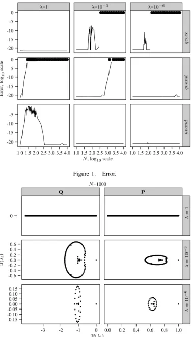
N=1000 ℜ(λl) ℑ ( λl ) 0 -0.6 -0.4 -0.20.0 0.2 0.4 0.6 -0.15 -0.10 -0.050.00 0.05 0.10 0.15 Q -3 -2 -1 0 P 0.0 0.2 0.4 0.6 0.8 1.0 λ = 1 λ = 10 − 3 λ = 10 − 6
Figure 3. Complex-plane plot of the eigenvalues of the matricesQandP forN= 1000. N=100 t,log10scale Probability , log 10 scale -10 -5 0 -40 -30 -20 -10 -60 -40 -20 0 qevec -1 0 1 2 3 4 5 uvand -1 0 1 2 3 4 5 λ = 1 λ = 10 − 3 λ = 10 − 6
Figure 4. Probabilitiesπj(t),j = {0,· · ·9} for theqevec anduvand methods forN = 100. Values obtained with Sharma’s formula are plotted with dashed lines.
and we assume that the initial state is j = 0. The system capacity (N), has been varied between 10 and 104 (note that the number of states of the Markov chain is N+ 1). In the interval [10,100] the transient solution was computed for all values ofN, since each computation took few seconds. In the interval (100,104] there were taken 20 points evenly spaced
in log scale (10 per decade). The service rate has been set to µ= 1and the arrival rate have been set to three different values: λ= 1,10−3 and10−6.
The methods are compared against the formula proposed by Sharma and Tarabia in [21]. Due to the combinatorial co-efficients of Sharma’s formula, its numerical evaluation gives very accurate results for values oftup to100s approximately.
In order to estimate the error for each of the methodsm=
{qevec, qvand, uvand}it has been proceed as follows.π0(m)(t) have been evaluated at 60 values oftevenly spaced in log scale in the range (10−1,102] (20 points per decade). All values π0(m)(t)<0 and π0(m)(t)>1 where considered as failed. If the number of failed points was larger than 12 (more than 20% of failed points), it was considered that the method failed. For the non-failed points,n, it was computed:
error(m)= 1 n n X i=1 (π(0m)(ti)−π (sh) 0 (ti))2 π0(sh)(ti) (33) whereπ(0sh)is the probability obtained with Sharma’s formula.
N,log10scale Computational time, log 10 scale 0 1 2 3 4 1.0 1.5 2.0 2.5 3.0 3.5 4.0 method qevec qvand uvand
Figure 5. Computational time.
N,log10scale Mean eigen values multiplicity 20 40 60 80 100 120 1.0 1.5 2.0 2.5 3.0 3.5 4.0 λ 1 10−3 10−6
Figure 6. Mean eigenvalues multi-plicity. N,log10scale Matrix size, log 10 scale 1.5 2.0 2.5 3.0 3.5 4.0 1.0 1.5 2.0 2.5 3.0 3.5 4.0 λ 1 10−3 10−6
Figure 7. V(P)matrix size in the uvandmethod. N,log10scale n ∗= q t ∗, log 10 scale 0 1 2 3 4 5 6 1.0 1.5 2.0 2.5 3.0 3.5 4.0 λ 1 10−3 10−6 k
Figure 8. Valuesn∗ =q t∗, and k=N+ 1.
Figure 1 shows the error obtained in each scenario. The failed points, or those points where the solver failed to compute the UC (because rounding errors made the numerical tool finding the matrix singular), are marked with a dot at error=1. Figure 2 shows the condition number of the matrix used to computed the UC: the Eigenvectors matrix forqevec, and the Vandermonde matricesV(Q)andV(P)forqvandand uvand respectively (see section VI). In figure 2 the points located aty= 1mark the scenarios where the solver failed to compute the UC. Both figures are in log-log scale.
Figure 1 shows thatqevec is very accurate forλ= 1. This is because Q is symmetric for λ = 1, and it is known that Eigenvectors method works very well in this case (see e.g. [5]). In fact figure 2 shows that the condition number forλ= 1in qevec is constant and equal to 1. For λ6= 1 figure 2 shows that the condition number for qevec increases rapidly with increasingN. In fact, the lower isλ, the less symmetric isQ,
and the smaller are the values of N for whichqevec is able to computed the UC. Regarding the method qvand, figure 2 shows that the condition number increases rapidly with N for λ= 1 and 10−3, explaining the bad results observed for
this method in figure 1 for these values ofλ. This is because the eigenvalues of Q are out of the unit circle, and thus, the
norm of V(Q) increases rapidly with increasingN. This can
be observed in figure 3. This figure shows a complex-plane plot of the eigenvalues obtained with the numerical tool for the matrixQ, and the uniformized matrixP, forN = 1000.
Finally, figure 1 shows thatuvandis the only method that succeeds to compute the transient solution for all values ofλ andN. Figure 2 shows that the condition number ofV(P)is
between1020and1025for most of the values ofN. This is a
large condition number, however, figure 1 shows that the error for uvandis very low when λ6= 1.
To explain what happens withuvandwhenλ= 1, figure 4 depicts the probabilitiesπ(jm)(t),j= 0,· · ·9for the scenarios m = {qevec, uvand} and λ = {1, 10−3, 10−6
} when N = 100. In the intervalt∈[10−1, 102] the values obtained
with Sharma’s formula are plotted with dashed lines (note that the error depicted in figure 1 was computed in this interval). Figure 4 shows that π(juvand)(t) starts diverging when t is approximately 100 s. In fact, the error observed in figure 1 in uvand method for N between 10 and 102.5, is because there were taken some samples of πj(uvand)(t) in the region
where it diverges. For N > 102.5 the error is negligible
because the divergence of πj(uvand)(t)starts after the interval considered in the error estimation. This instability is discussed in section VIII.
Figure 5 shows the computation time in seconds for each method in the scenario with λ= 1, for the points where the numerical tool was able to compute the UC. It can be seen that for values ofN up to 102.5, approximately,qevec is the
fastest method. However, for larger values ofN the methods qvandanduvandare faster. This is motivated by the cost of computing the eigenvectors in theqevecmethod.
An additional advantage of the uvand method is the reduction of the required UC in some scenarios. This is shown in figures 6 and 7, which respectively plot the mean multiplicity of the eigenvalues computed by the numerical tool, and the V(P) matrix size (number of required UC, k, in the uvand method). In the extreme case (λ = 10−6 and
N = 104) figure 6 shows that the numerical tool yielded a
mean multiplicity of the eigenvalues equal to 120.5. Figure 7 shows that only 155 different UC were needed to compute the transient solution for this scenario. This result comes from the fact that the maximum multiplicity was limited toM = 5(see remark 5),
VIII. DISCUSSION
The intuitive explanation of the divergence of πj(uvand)(t) whenλ= 1 is the following. The Uniformized Vandermonde method can be interpreted as a fitting of the points of the uniformized probabilities, πj(P)(n), to the samples Pn, for
n = 0,1,· · ·k−1. In the interval where these samples are taken, the corresponding probabilities obtained for πj(Q)(t) are very accurate (recall from 4 that π(jP)(n) converges to πj(Q)(t)at the pointsn=q t). Ifπ(jP)(n)reaches the stationary distribution within the sampling interval n = 0,1,· · ·k−1, then uvand is very accurate for all values of t. This comes from the fact that the UC would have been computed taking into account the evolution of the chain up to the stationary regime. This fact holds forλ={10−3, 10−6}, but forλ= 1 the probabilitiesπj(Q)(t)converge to the stationary regime very slowly. Note that this is an expected result, since an M/M/1 queue is null recurrent forρ=λ/µ= 1. Thus, forN → ∞the duration of the transient regime→ ∞. We conclude that the method is expected to give accurate results as far the duration
of the transient regime of the chain is not much larger than the interval used to compute the UCs.
In order to check this condition it can be proceed as follows. The duration of the transient regime of πj(Q)(t) is related with the second smallest eigenvalue, in modulus: λ∗l = minl,λl6=0|λ
(Q)
l |. If λ∗l is close to 0, then e−
λ∗lt will
vanish for large t, thus, with a long transientregime. Define
n∗=q t∗= α q minl,λl6=0|λ
(Q)
l |
(34) Note that e−λ∗lt∗ = e−α. Thus, t∗ is an estimation of the time whereπ(jQ)(t)reaches the its stationary regime. Note that at time t∗ all coefficients of π(jQ)(t), but the stationary one, have vanished by at least e−α. Figure 8 depicts the values of
n∗=q t∗given by equation (34), forα= 0.1, andk=N+1. The figure confirms that π(jQ)(t) converges very fast to its stationary regime for λ={10−3, 10−6
}, but very slowly for λ= 1. For instance, whenN = 100,n∗ ={413,0.26,0.25} forλ={1, 10−3, 10−6
}, respectively. In fact, figure 8 shows that for λ= 1, the duration of the transient regime becomes larger thank for aroundk= 25.
We conclude with the following rule to estimate the stability of the method: Compute n∗ given by (34). If n∗≤k (recall the k is the number of UC to be determined), then method is expected to give a very accurate close formula for πj(Q)(t). Otherwise, πj(Q)(t)may diverge when for values of tk/q. The divergence problem observed for the uvand method claims for discussion. First note that, due to rounding errors, none method is completely stable [5]. The best method de-pends on the properties of the rate matrix. This comes clear from the numerical results, where the eigenvectors method was always stable for λ = 1, but failed rapidly otherwise. Methods based on matrix series, as the uniformization method, have shown to be very robust, and may be more general than the method proposed in this paper. Nevertheless, the close formula provided by the uvand method has important advantages. For instance, once the eigenvalues and the UCs have been computed, it can be evaluated much faster than a matrix series. Additionally, it can save memory, since at most 2N values need to be stored (the eigenvalues and the UCs), instead of theN2 values of the rate matrix.
IX. CONCLUSIONS
In this paper are investigated the class of methods based on theundetermined coefficientsapproach to compute a close form transient solution of continuous time Markov chains (CTMCs). This approach consists on guessing the solution in terms of a set of undetermined coefficients (UC), and derive a system of equations that computes them. The well known Eigenvectors method belongs to this class, but it has the drawback that it cannot be used to solve defective matrices, which are likely to occur in practice due to rounding errors.
Another approach consists of applying the undetermined coefficients approach directly to the transient solution of a Markov chain in terms of its eigenvalues. Doing this way it is
obtained a Vandermonde system of equations, and we refer to it as theVandermonde Method. This method has the advantage that it can be used even for chains having a defective matrix. However, the Vandermonde system of equations obtained for CTMCs may be ill-conditioned for chains having a large number of states.
To solve this problem, a mapping is derived between a close form transient solution of a CTMC, and a close form transient solution of one of its uniformized discrete time Markov chains (DTMCs). We exploit this mapping by proposing a new approach to compute the transient solution of CTMCs by using the Vandermonde method with one of its uniformized DTMCs: one having a well conditioned matrix. We refer to this approach as the Uniformized Vandermonde (UV) method. The benefits of this new method are analyzed through extensive numerical results. The method is simple to implement and numerical results show that it is rather general, giving an accurate solution in most scenarios where it was tested. Furthermore, a rule of thumb is given to estimate when the method may diverge.
APPENDIX A. DERIVATION OF∂nπj(0)
∂tn
In order to solve the system of equations (16) we need to compute the derivatives of functions of the type:
πk−1(t) = (a0+a1t+· · ·+ak−1tk−1)eλ t (35)
In this appendix a general formula is obtained. This is neces-sary to implement a script for solving the system of equations given by (16). Start by noting that:
∂πk−1(t)
∂t = [(λa0+a1) + (λa1+ 2a2)t +· · · (λak−2+ (k−1)ak−1)tk−2+λak−1tk−1)
eλ t (36)
which is again a polynomial in t of degree (k−1) times an exponential. Let identify the coefficients of the polynomial associated with ∂nπk−1(t)
∂tn byam(n),m= 0,· · ·(k−1), and
define the column vector a(n) =
a0(n) · · · ak−1(n).
Note that a(0) = a0 · · · ak−1
. By induction it can be easily obtained thata(n)obeys the systems of linear difference equationsa(n+ 1) =A a(n), where: Ak×k = λ 1 0 0 · · · 0 λ 2 0 · · · 0 0 λ 3 · · · · · · (37) This system has the solutiona(n) =Ana(0). WritingA=
λI+U, where Uis the matrix:
Uk×k= 0 1 0 0 · · · 0 0 2 0 · · · 0 0 0 3 · · · · · · (38)
we have that: An = n X m=0 n m λn−mUm (39)
whereU0=IandUmis a matrix with themupper diagonal equal to: m!,(m+ 1)! 1! , (m+ 2)! 2! , n−k · · ·, (k−1)! (k−m−1)! (40)
for m= 1,· · ·k−1, andUm=0form≥k. Note now that: ∂nπ
k−1(0)
∂tn =a0(n) (41)
which is the first component of the vector a(n). Thus, us-ing (39) and (40) we obtain:
∂nπk−1(0) ∂tn = k−1 X m=0 n m m!λn−mam= k−1 X m=0 nmλn−mam (42) where nm =n(n −1)· · ·(n−m+ 1), i.e. m-permutations of n, withnm= 0 forn < m, and00= 1.
Letc(jl,m)(n)be the coefficient of the equationn,0≤n≤ k−1 of the system of equations (16) that multiplies the UC a(jl,m) ofπj(t). Using (42) we conclude that:
c(jl,m)(n) =nmλnl−m (43) B. DERIVATION OFq(l,m)(t)
In equation (22) we need to compute the following summa-tion for the eigenvalues with multiplicity higher than 1:
Sm= ∞ X n=0 (q t)n n! (λ (P) l ) nnm= ∞ X n=0 xn n! n m, m ≥1 (44) wherex=q t λ(lP). Clearly, S0=ex (assuming nm= 1,∀n
for m= 0) and, Sm= ∞ X n=0 xn n! n m=x ∞ X n=1 (n−1 + 1)m−1 x n−1 (n−1)! =x ∞ X n=1 m−1 X i=0 m −1 i (n−1)i x n−1 (n−1)! = x m−1 X i=0 m −1 i Si, m≥1 (45)
From (45) it can be easily derived thatSmare eq t λ
(P) l times polynomials intof degreem:Sm=eq t λ (P) l q(l,m)(t), where: q(l,m)(t) = m X i=1 q(im)(q λ(lP))iti (46)
with coefficients qi(m) given by the recurrence relation: q(im)= ( 1, i= 1 Pm−1 k=i−1 m−1 k qi(−k)1, i= 2,· · ·m (47) REFERENCES
[1] R. A. Marie, A. L. Reibman, K. S. Trivedi, Transient analysis of acyclic Markov chains, Performance Evaluation 7 (3) (1987) 175–194. [2] G. Hj´almt`ysson, W. Whitt, Periodic load balancing, Queueing systems
30 (1) (1998) 203–250.
[3] P. Heegaard, K. S. Trivedi, Network survivability modeling, Computer Networks 53 (8) (2009) 1215–1234.
[4] A. Ramesh, K. S. Trivedi, Semi-numerical transient analysis of markov models, in: ACM-SE 33: Proceedings of the 33rd annual on Southeast regional conference, ACM, 1995, pp. 13–23.
[5] C. Moler, C. Van Loan, Nineteen dubious ways to compute the expo-nential of a matrix, twenty-five years later, SIAM review 45 (1) (2003) 3–49.
[6] D. Dormuth, A. Alfa, Two finite-difference methods for solving MAP(t)/PH(t)/1/K queueing models, Queueing systems 27 (1) (1997) 55–78.
[7] A. L. Reibman, K. S. Trivedi, Numerical transient analysis of markov models, Comput. Oper. Res. 15 (1) (1988) 19–36.
[8] H. Nabli, Transient and asymptotic analysis of general markov fluid models, Queueing Systems 47 (3) (2004) 283–304.
[9] W. J. Stewart, Introduction to the numerical solution of Markov chains, Princeton University Press, 1994.
[10] S. Elaydi, An Introduction to Difference Equations, 3rd Edition, Springer, 2005.
[11] M. Vidyasagar, A novel method of evaluating eAt in closed form, Automatic Control, IEEE Transactions on 15 (5) (1970) 600 – 601. doi:10.1109/TAC.1970.1099568.
[12] S. Karlin, H. Taylor, A first course in stochastic processes, Vol. 697, Academic press New York, 1975.
[13] W. H. Jr, J. Fillmore, D. Smith, Matrix Exponentials: Another Approach, SIAM review 43 (4) (2001) 694–706.
[14] I. Leonard, The matrix exponential, SIAM Rev. 38 (3) (1996) 507–512. [15] J. A. Sjogren, Closed-form solution of decomposable stochastic models,
Computers & Mathematics with Applications 23 (12) (1992) 43–67. [16] ˚A. Bj¨orck, V. Pereyra, Solution of vandermonde systems of equations,
Mathematics of Computation 24 (112) (1970) pp. 893–903.
[17] G. Stewart, The Decompositional Approach to Matrix Computation, Computing in Science & Engineering 2 (1) (2002) 50–59.
[18] W. Grassmann, J. Tavakoli, Transient solutions for multi-server queues with finite buffers, Queueing Systems 62 (1) (2009) 35–49.
[19] R Development Core Team, R: A Language and Environment for Statistical Computing, R Foundation for Statistical Computing, Vienna, Austria, ISBN 3-900051-07-0 (2010).
URL http://www.R-project.org/
[20] M. Malhotra, J. K. Muppala, K. S. Trived, Stiffness-tolerant methods for transient analysis of stiff markov chains, Microelectronics and Reliability 34 (1994) 1825–1841.
[21] O. Sharma, A. Tarabia, A Simple Transient Analysis of an M/M/1/N Queue, The Indian Journal of Statistics (2000) 273–281.
[22] W. J. Stewart, MARCA Models: A Collection of Markov Chain Models. URL http://www4.ncsu.edu/∼billy/MARCA Models/MARCA Models. html
[23] W. Feller, An Introduction to Probability Theory and Its Applications, Vol. 1, 3rd Edition, Wiley, 1968.