TI 2005-035/3
Tinbergen Institute Discussion Paper
Human Capital and Optimal
Positive Taxation of Capital
Income
Bas Jacobs
1A. Lans Bovenberg
21University of Amsterdam, Tinbergen Institute, and European University Institute; 2 CentER, University of Tilburg, Erasmus University Rotterdam, Netspar, and CEPR.
Tinbergen Institute
The Tinbergen Institute is the institute for economic research of the Erasmus Universiteit Rotterdam, Universiteit van Amsterdam, and Vrije Universiteit Amsterdam.
Tinbergen Institute Amsterdam Roetersstraat 31
1018 WB Amsterdam The Netherlands
Tel.: +31(0)20 551 3500 Fax: +31(0)20 551 3555 Tinbergen Institute Rotterdam Burg. Oudlaan 50
3062 PA Rotterdam The Netherlands
Tel.: +31(0)10 408 8900 Fax: +31(0)10 408 9031
Please send questions and/or remarks of non-scientific nature to driessen@tinbergen.nl. Most TI discussion papers can be downloaded at http://www.tinbergen.nl.
Human Capital and Optimal Positive
Taxation of Capital Income
∗
Bas Jacobs
†and A. Lans Bovenberg
‡¦April 5, 2005
Abstract
This paper analyzes optimal linear taxes on capital and labor incomes in a life-cycle model of human capital investment, financial savings, and labor supply with heteroge-nous individuals. A dual income tax with a positive marginal tax rate on not only labor income but also capital income is optimal. The positive tax on capital income serves to alleviate the distortions of the labor tax on human capital accumulation. The optimal marginal tax rate on capital income is lower than that on labor income if savings are elastic compared to investment in human capital; substitution between inputs in human capital formation is difficult; and most investments in human capital are verifiable. Numerical calculations suggest that the optimal marginal tax rate on capital income is close to the tax rate on labor income.
Keywords: human capital, labor income taxation, capital income taxation, life cy-cle, education subsidies.
JEL codes: H2, H5, I2, J2.
1
Introduction
The case for zero taxation of capital income is quite strong in models with infinitely lived individuals. In particular, this zero-tax result holds for quite general specifications of prefer-ences (see Chamley, 1986; and Judd, 1985, 1999). Erosa and Gervais (2002) analyze optimal capital income taxes in life-cycle models rather than models with infinitely lived individuals.
∗The authors thank Rick van der Ploeg, Søren Bo Nielsen, seminar participants at the University of
Ams-terdam, the London School of Economics, and members of the CES-Ifo area conference on Public Economics, May 7–9, 2004, M¨unchen for useful comments and suggestions. Bas Jacobs gratefully acknowledges financial support from the NWO Priority Program ‘Scholar’ funded by the Netherlands Organization for Sciences. This paper previously circulated under the title “Optimal Capital Income Taxation with Endogenous Human Capital Formation”.
†European University Insitute, University of Amsterdam, and Tinbergen Institute. E-mail:
bas.jacobs@iue.it. ‡University of Tilburg, CentER, Erasmus University, OCfEB, and CEPR. E-mail:
a.l.bovenberg@uvt.nl. ¦Corresponding author: CentER, University of Tilburg, P.O. Box 90153, 5000 LE
They show that optimal capital taxes are not necessarily zero if utility is not additively sep-arable in consumption and leisure, or, if utility does not feature weak separability between leisure and homothetic sub-utility over consumption. Building upon Ramsey-Corlett-Hague intuition, Erosa and Gervais (2002) demonstrate that optimal capital taxes are positive if leisure and consumption are more complementary later in life than they are earlier in life. See also Bernheim (2002) for a more elaborate discussion.1
Another strand of literature stresses the role of incomplete markets rather than life-cycle issues. Aiyagari (1995) and Golosov, Kocherlakota and Tsyvinski (2004) derive optimal taxes on capital incomes in infinitely lived agent models in the presence of incomplete capital or insurance markets. Both papers find that capital income is optimally taxed at positive rates. Intuitively, positive capital income taxes redistribute resources from unconstrained towards liquidity constrained phases in the life cycle and from high income states towards low income states of nature. Hence, a positive tax on capital income helps to complete the missing capital and insurance markets.
We establish another case for positive capital taxes by allowing for endogenous human capital formation in a life-cycle model.2 In contrast to the papers mentioned above, our
case for positive capital income taxes relies neither on non-separable preferences nor market failures.3 Indeed, in our setting with weakly separable preferences and perfect financial
markets, optimal capital taxes would be zero in the absence of human capital formation. To develop our case, we formulate a simple three period life-cycle model of labor supply, human capital and financial savings with heterogenous agents who differ in their abilities to acquire human capital. Individuals invest in human capital in the first period of their lives. In the second period, they work and consume leisure. They retire and consume all their assets in the last, third period.
We demonstrate that positive capital taxes are optimal to alleviate the distortionary effects of the labor tax on investments in human capital. Whereas labor taxes encourage individuals to substitute human by financial assets, the capital tax offsets these distortions in the composition of saving. Since capital income taxes distort the overall level of saving, the optimal capital tax strikes a balance between distorting the composition and the level of saving. Indeed, the government faces a fundamental trade-off between efficiency in human capital formation and allocative efficiency in the intertemporal allocation of consumption. The optimal tax rate on capital income is relatively large compared to the tax on labor income if aggregate saving is inelastic compared to learning, so that learning distortions dominate saving distortions.
Optimal taxes on capital are positive because the government cannot employ subsidies or tax deductions for human capital investments to offset all the distortions of the labor
1In life-cycle models with heterogenous households, Ordover and Phelps (1979) and, Atkinson and Sandmo
(1980) showed earlier that the optimal capital tax is zero if leisure is weakly separable from consumption.
2The literature on the optimal taxation of capital income typically abstracts from human capital
accu-mulation. See Boskin (1975) and Heckman (1976) for earlier treatments of the effects of capital income taxes on human capital formation. These treatments are not put in an optimal tax setting.
3All the papers mentioned, including our own, assume that the government can commit to announced
policies. A lack of commitment can also result in positive capital income taxes (see Kydland and Prescott, 1980; and, Fischer, 1980). We show that capital income taxes are optimally positive even if the government can credibly commit to tax policies.
income tax on human capital formation. Non-verifiability of human capital investments excludes these more direct instruments. Non-verifiability of learning is analogous to the non-verifiable nature of work effort in the optimal tax literature.4 Direct educational expenditures
on books, computers and traveling are important examples of non-verifiable investments in human capital. Moreover, costs of effort while enrolled in education, such as studying hard, sacrificing leisure activities, preparing exams, are important immaterial costs that the government cannot verify easily.5 In contrast, the indirect costs of education, forgone labor
earnings while enrolled in education, are in effect deductible from labor taxation as lower labor earnings reduce the labor tax bill. Tuition costs, however, cannot be deducted for income-tax purposes in many countries, so that these costs are effectively non-verifiable.
We demonstrate that the government optimally taxes capital if at least some investments in human capital are non-verifiable. Only if it can verify all investments in education (so that it can subsidize these costs), the government does not have to rely on capital income taxes to alleviate the labor tax distortions on learning. Distortions in the aggregate level of saving can thus be avoided. This rather special ‘knife-edge’ case explains the findings of some recent papers that the optimal capital tax is zero in the presence of human capital accumulation (see Judd 1999; and Bovenberg and Jacobs, 2001).6 Trostel (1993) estimates
that the share of non-verifiable costs of education approaches as much as one quarter of total costs, even though he does not include the effort costs of education. Our numerical simulations show that optimal tax rate on capital income approaches that on labor incomes, even if non-verifiable investments account for only 20% of total investments in human capital. The case for substantially positive capital income taxes does not directly depend on the redistributive preferences of the government. It relies only on the presence of positive labor income taxes. In our model, distortionary labor taxation increases with a stronger distribu-tional preference of the government. Hence, in contrast to representative agent models (see, e.g. Atkinson and Sandmo, 1980; Nielsen and Sørensen, 1997; and Judd, 1999), we do not have to arbitrarily exclude lump-sum taxes as a policy instrument to prevent the optimal tax problem from becoming trivial.
The rest of this paper is organized as follows. Section 2 describes individual behavior. Section 3 derives optimal tax policy if all educational efforts are non-verifiable. Subsequently, section 4 introduces verifiable educational efforts, which the government can subsidize. Sec-tion 5 performs some numerical simulaSec-tions and demonstrates that a synthetic income tax is roughly optimal under a wide range of parameter values. Section 6 concludes and discusses the policy implications of the analysis. Four appendices contain the technical details of our analysis.
4The literature on optimal labor taxation follows Mirrlees’ (1971) pioneering analysis by assuming that
the government cannot verify work effort and individual ability, thereby excluding individualized lump-sum taxes.
5Education may also generate immaterial benefits, such as the fun of studying, nicer jobs, additional
status, more freedom of occupational choice, et cetera. Immaterial benefits, however, are typically much less important than immaterial costs in view of the observed high returns on (higher) education, which exceed returns on safe investments and approach those on equity. Whereas these high returns can be due to market failures, they probably also compensate investors for non-pecuniary costs that exceed non-pecuniary benefits (see also Judd, 2000; and, Palacios-Huerta, 2003).
6Nielsen and Sørensen (1997) assume an exogenously given positive capital tax. If the government would
2
The model
2.1
Preferences and technologies
We consider a partial equilibrium three-period life-cycle model without uncertainty. Before-tax wage rates and interest rates are exogenously fixed.7 A mass of agents with unit measure
lives for three periods. In the first period, agents supply unskilled labor and devote resources to learning. In the second period, agents supply skilled labor and spend time on leisure, which can be interpreted as early retirement. Individuals are retired in the third period and consume all their assets. Perfect capital markets allow individuals to freely transfer resources across the three periods.8
Individuals are heterogeneous in exogenous ability n. The cumulative distribution of ability is F(n). f(n) represents the corresponding density function, which is continuously differentiable and strictly positive on the support [n, n],n, n > 0. The government knows the distribution of abilities, but does not observe individual ability. Accordingly, it cannot levy individual-specific lump-sum taxes to redistribute incomes, but must rely on distortionary taxes instead.
In the first period of their lives, individuals invest en in education. Initially, we assume
that the government cannot observe any of these educational inputs so that it cannot subsi-dize these investments. Educational investment therefore consists only of direct expenditures and effort costs. Section 4 shows that our main results continue to hold if verifiable costs of education are allowed for as long as some non-verifiable costs remain.9 For analytical
convenience, we abstract from first-period consumption and leisure demands.10
Ability n can be viewed as the productivity of education, so that more able individuals produce more human capital with the same educational effort. The production function for human capital is homothetic:
hn =nφ(en)≡n(en)β, (1)
wherehndenotes human capital of agentn. Human capital accumulation exhibits decreasing
returns with respect to educational effort en (i.e., β < 1). Ability and educational
invest-ments are complementary inputs in producing human capital (i.e., ∂2hn
∂en∂n =β(en)β−1 ≥0).
In the second period, human capital is supplied to the labor market in the form of skilled labor. Gross second-period labor income zn is the product of the number of efficiency units
of human capital, hn, and hours worked ln, i.e.,zn ≡hnln=nφ(en)ln.11 In the third period,
7The model can thus be viewed as a model of a general equilibrium small open economy in which the
international capital market fixes the real interest rate.
8Cameron and Heckman (2001) and Carneiro and Heckman (2002) argue that liquidity constraints are
only of minor importance empirically.
9Bovenberg and Jacobs (2005) explore optimal labor tax and education policies in the presence of both
verifiable and non-verifiable inputs into human capital formation. They abstract, however, from capital income taxes.
10First-period consumption and leisure do not affect our main result that optimal capital taxes are positive.
The presence of first-period consumption, however, would exacerbate the welfare costs of positive capital income taxes. Endogenous first-period leisure demands would increase the distortionary costs of the labor tax. Hence, the effect of first-period consumption and leisure on the optimal structure of labor and capital taxes is ambiguous.
individuals are retired and finance their consumption by selling the financial assets they have accumulated in the second period.12
Individuals feature a common, concave, and twice differentiable utility function defined over consumption in the second periodcn
1, leisure`n ≡1−ln, and consumption when retired cn
2:
u(v(cn
1, cn2), `n), (2)
whereuc1uc2, u` >0, anduc1c1, uc2c2, u`` ≤0. The sub-utility function v(c
n
1, cn2) is homothetic
and weakly separable from leisure `n. We employ this particular utility function because
it most clearly shows how endogenous human capital formation affects the optimal capital income tax. Indeed, with this utility function, the optimal capital income tax would be zero in the absence of human capital formation (see Bernheim, 2002; and, Erosa and Gervais, 2002).
2.2
Budget constraints
The first-period budget constraint is
−an
1 =en. (3)
First-period saving an
1 is negative because individuals borrow to finance their education. In
the second period, individuals consume, work, pay off their first-period debts and save for retirement. Hence, the second-period budget constraint amounts to
cn
1 = (1−t)lnnφ(en) +Ran1 −an2 +g, (4)
whereR ≡1 + (1−τ)r,r stands for the exogenous real interest rate, and τ denotes the tax rate on capital income. The lump-sum transfer g and the marginal tax rate t characterize the linear labor tax.
The individual consumes all assets in the third period:
cn
2 =Ran2. (5)
We arrive at the life-time budget constraint by substituting the first-period and third-period budget constraints (i.e. (3) and (5), respectively) into the second-third-period budget constraint (4) to eliminate an 1 and an2: cn1 +c n 2 R = (1−t)l nnφ(en)−Ren+g. (6)
at unity. Alternatively, abilityncan be interpreted as the skill in second-period work corresponding to the wage rate per efficiency unit of labor. In that case,φ(en) (instead ofnφ(en)) defines the efficiency units of
labor (or human capital) per hour worked. Dur and Teulings (2001) investigate optimal education policies in a general equilibrium model in which different labor types are imperfect substitutes in labor demand.
12We include a third period to allow high ability agents to save more than low ability agents do. In the
absence of a third period, high ability agents would feature the lowest life-time savings, because they borrow more than low ability agents to finance their education in the first period. Our main results, however, do not rely on any particular relationship of financial savings with ability.
2.3
Individual optimization
Individuals maximize their utilities by choosing cn
1,cn2,`n, and en, subject to their life-time
budget constraints, and taking the policy instruments of the government as given.13 The
resulting first-order condition for the optimal choice of en amounts to
(1−t)lnnφ0(en) = 1 + (1−τ)r=R. (7) Marginal benefits of education (the left-hand side) should equal marginal costs (the right-hand side). The labor tax harms learning by depressing marginal benefits (sinceφ00(en)<0).
The capital income tax, in contrast, boosts education because it raises the present value of investments in human capital by reducing the rate of return on alternative investments R.
Indeed, capital income taxes induce individuals to substitute human capital for financial savings in their portfolio of human and financial assets.
The first-order condition for en (7) and the production function of human capital (1)
imply that second-period gross labor income zn is proportional to en:
zn=lnnφ(en) = R
(1−t)βe
n, (8)
The proportionality factorR/(1−t)β does not depend on ability n and is thus the same for all agents.
The first-order condition for labor supply amounts to
u` uc1
=wn≡(1−t)nφ(en), (9) while the Euler equation for savings is
uc1
uc2
= 1 + (1−τ)r=R. (10) Substituting the link between en and zn (8) into the life-time budget constraint (6), we
find that the discounted value of life-time consumptioncn
1+
cn
2
R is linear in gross income (and
in view of (8) also linear in learning):
cn 1 + cn 2 R = (1−β)(1−t)z n+g. (11)
Weak separability between leisure and consumption in utility and homotheticity ofv(cn 1, cn2)
imply that the shares of third- and second-period consumption in after-tax labor income do not depend on ability n, i.e.,
ω ≡ c
n
2/R
(1−β)(1−t)lnnφ(en) +g, (12)
13The government sets policy before agents determine their behavior. In view of its distributional
pref-erences, the government faces an incentive to change its policy after the private sector has accumulated human and financial capital. The government thus must have access to a commitment technology (e.g., due to reputational considerations).
1−ω ≡ c n 1
(1−β)(1−t)lnnφ(en) +g. (13)
The second-order conditions for a utility maximization imply (see Appendix A)
µn≡1−β(1 +²n)>0, (14)
where ²n≡ ∂ln
∂wnw n
ln, denotes the compensated wage elasticity of labor supply with respect to
the after-tax wagewn ≡(1−t)nφ(en).14 Decreasing returns in human capital accumulation
(β < 1) are not sufficient for the second-order condition to be met because of the positive
feedback between human capital and labor supply. In particular, more learning raises the wage rate. The associated substitution effect boosts labor supply, which, in turn makes learning more attractive. In order to prevent corner solutions, decreasing returns in the production of human capital must offset this positive feedback effect, which rises with the compensated wage elasticity of labor supply ²n.
2.4
Government
The government taxes labor at rate t and capital incomes at rate τ to finance exogenously given public spending Λ and the endogenous uniform lump-sum transferg. The fundamental informational assumptions are that the government must be able to verify aggregate labor incomesRnnlnnφ(en)dF(n) and aggregate capital incomes Rn
n r ³ an 1 + an 2 1+r ´ dF(n).
The government budget constraint reads as
Z n n · tlnnφ(en) +τ r µ an 1 + an 2 1 +r ¶ −g−Λ ¸ dF(n) = 0. (15) The government budget constraint can be written in terms oft and R by using the first and third-period households budget constraints (3) and (5) to eliminate an
1 and an2: Z n n · tlnnφ(en) +Ren+cn2 R −(1 +r)e n− cn2 1 +r −g−Λ ¸ dF(n) = 0. (16) The government’s budget is fully funded and the government can freely borrow and lend at the capital market at rate r.15
The government maximizes a social welfare function Γ defined over individuals’ indirect utilitiesυ(g, t, R, n):
Γ≡
Z n
n
Ψ(υ(g, t, R, n))dF(n), (17)
where Ψ0 >0, and Ψ00≤0. With Ψ0 = 1, the social welfare function is utilitarian.
14The compensated tax elasticity of labor supply (²n/µn) exceeds the compensated wage elasticity of labor
supply²n.The reason is that the tax rate depresses the after-tax wage rate not only directly by raising the
tax wedge, but also indirectly by reducing human capital investments and thus the before-tax reward for each additional unit of labor effort ln.We can express the compensated elasticities of the endogenous variables
with respect to the policy parameters in terms of²n by totally differentiating the first-order conditions (7),
(9), and (10) (see Appendix B for the derivations).
15As in Nielsen and Sørensen (1997), one can interpret our model as the steady state of an overlapping
generation’s economy. In that case, our optimal taxes are equivalent to the optimal taxes of a Pareto efficient tax reform where the government insulates the existing generations from the transition by employing public-debt policy.
3
Optimal taxation
The Lagrangian L for maximizing social welfare is given by max {g,t,R}L = Z n n Ψ (υ(g, t, R, n))dF(n) + (18) η Z n n · tnlnφ(en) +Ren+c n 2 R −(1 +r)e n− cn2 1 +r −g−Λ ¸ dF(n),
where η represents the Lagrange multiplier of the government budget constraint. We apply Roy’s lemma (using (6)) to derive the following properties:
∂υ(g, t, R, n) ∂g =λ n, (19) ∂υ(g, t, R, n) ∂t =−λ nlnnφ(en), (20) ∂υ(g, t, R, n) ∂R =λ n µ −en+ c n 2 R2 ¶ , (21)
where λn denotes private marginal utility of second-period income for an individual with
ability n.
3.1
Optimal lump-sum transfer
The first-order condition for maximizing the Lagrangian (18) with respect to the lump-sum transfer g amounts to ∂L ∂g = Z n n · Ψ0λn−η+η∆∂en ∂g +ηtnφ(e n)∂ln ∂g +η τ r (1 +r)R ∂cn 2 ∂g ¸ dF(n) = 0, (22) where we used Roy’s lemma (19). ∆≡ tnlnφ0(en)−τ r=¡ t
1−t ¢
R−τ r represents the total tax wedge on investments in human capital (where the second equality is derived by using the first-order condition for learning (7)).
By defining the net social marginal value of income of an individual with ability n (in-cluding the effect on the tax base)
bn≡ Ψ 0λn η + ∆ ∂en ∂g +tnφ(e n)∂ln ∂g + τ r (1 +r)R ∂cn 2 ∂g , (23)
we can write first-order condition (22) as ¯
b ≡
Z n
n
bndF(n) = 1. (24)
The average social marginal benefits of a higher g (i.e., the left-hand side of (24)) should equal the costs in terms of a higher g (i.e., last the right-hand side of (24)).
In order to facilitate the discussion of the optimal tax schedules below, we define the so-called distributional characteristic ξ of labor income
ξ≡ Rn n(1−bn)zndF(n) Rn n zndF(n) Rn n bndF(n) , (25)
as the negative normalized covariance between the social value the government attaches to income of a particular abilitybn and gross second-period labor incomezn (see also Atkinson
and Stiglitz (1980)). This covariance coincides with the normalized covariances of the welfare weights bn with learning en because labor income zn is proportional to education en (see
(8)). A positive distributional characteristic ξ implies that the base of the labor tax is larger for high-ability agents (who feature relatively low welfare weights) than for low-ability agents (who feature relatively high welfare weights), so that taxing labor income yields distributional benefits. The magnitude of the distributional characteristic depends not only on the correlation between ability and the tax base, but also on the correlation between ability and the welfare weights. Indeed, a zero distributional characteristic implies either that the government is not interested in redistribution (so that the welfare weight bn is the
same for alln) or that all ability types feature the same labor income (taxable income is the same for all n).
3.2
Optimal labor income tax
The first-order condition for maximizing the Lagrangian for social welfare (18) with respect tot is given by ∂L ∂t = Z n n [−Ψ0λnnlnφ(en) +ηnlnφ(en)]dF(n) + (26) Z n n η · ∆∂e n ∂t +tnφ(e n)∂ln ∂t + τ r (1 +r)R ∂cn 2 ∂t ¸ dF(n) = 0,
where we used Roy’s lemma (20). We substitute the Slutsky equations, and use the definition of bn (see (23)) to obtain (see Appendix C)
ξ = −∆ Rβε¯et+ µ t 1−t + τ r (1 +r) ω κ ¶ ¯ εlt (27) = ∆β R µ 1 +² µ ¶ + µ t 1−t + τ r (1 +r) ω κ ¶ µ ² µ ¶ ,
where κ is the degree of homogeneity of the sub-utility function v(cn
1, cn2), and εnqt ≡ ∂q
n
∂t 1−qt
(forqn =en,ln,cn
2) are the compensated elasticities with respect to the labor tax. A bar
de-notes an income-weighted average of a skill-specific variable (i.e., ¯ε≡RnnεnzndF(n)/Rn
n zndF(n),
where εn is a variable that depends on ability).
The interpretation of the optimal labor tax (27) is as follows. The distributional benefits of a higher tax rate (ξ) (i.e. the left-hand side of (27)) should correspond to the additional first-order welfare losses as a result of the higher tax rate (i.e. the right-hand side of (27)).
These welfare losses arise because of first-order impacts on the learning distortion ∆ and the labor-supply distortion t
1−t + (1+τ rr)ωκ. The capital tax τ features in the labor-supply
distortion because the capital tax acts as an implicit tax on labor income by taxing retirement consumption as one of the uses of second-period labor income. In this way, a capital tax induces cross-substitution away from second-period consumption towards leisure.
In the absence of capital income taxes (i.e., τ = 0 so that ∆ = t
1−tR), the optimal
marginal tax rate on labor income is
t 1−t = ξ ³ ² µ ´ +β ³ 1+² µ ´. (28)
This expression illustrates the fundamental trade-off between equity and efficiency. If redis-tributional concerns become more important (as indicated by a larger disredis-tributional charac-teristic ξ), the optimal marginal tax rate rises (ceteris paribus the income-weighted elastic-ities). The denominator of (28) represents the distortionary costs of redistributive taxation in terms of the tax elasticity of total labor income. The first income-weighted elasticity
³ ² µ
´
=−ε¯lt captures the distortionary effect of the marginal labor tax rate on labor supply
and thus the base of the labor tax. The second term in the denominator β ³
1+² µ
´
= −βε¯et
stands for the distortion of the labor tax on human-capital accumulation. If large compen-sated elasticities (in absolute value) indicate that redistributive taxes substantially distort labor supply and human capital accumulation, positive marginal taxes are costly and the optimal marginal labor tax is low (ceteris paribus the distributional characteristicξ).
Expression (28) indicates that endogenous human capital formation (β > 0) raises the effective elasticity of the tax base in two distinct ways.16 First, due to positive feedback effects
with labor supply, endogenous learning raises the absolute value of the effective elasticity of labor supply (−ε¯lt ≡ µ²) by loweringµn≡1−β(1 +²n). Second, labor taxes distort not only
labor supply but also investments in human capital. The term β ³
1+² µ
´
captures this latter distortionary effect.
3.3
Optimal capital income tax
Maximization of social welfare (18) with respect to the capital income tax yields the following first-order condition: ∂L ∂R = Z n n · Ψ0λn µ cn 2 R2 −e n ¶ −η µ cn 2 R2 −e n ¶¸ dF(n) + (29) Z n n η · ∆∂en ∂R +tnφ(e n)∂ln ∂R + τ r (1 +r)R ∂cn 2 ∂R ¸ dF(n) = 0,
16With exogenous learning (i.e., β = 0), the model collapses to the standard model of optimal linear
income taxation with endogenous labor supply in which the optimal marginal taxtis given by t
1−t =ξ², see
where we used Roy’s lemma (see (21)). Substitution of the Slutsky equations and the defi-nition of bn (23) yields (see Appendix C)
(ω(1−β)−β)ξ+∆β R µ 1−ω² µ ¶ (30) = µ t 1−t + τ r (1 +r) ω κ ¶ (ω(1−β)−β) µ ² µ ¶ + τ r (1 +r)(ω(1−ω)σγ¯), whereσ ≡dlog (cn
2/cn1)/dlog(uc1/uc2) denotes the intertemporal elasticity of substitution in
consumption andγn ≡1−β+ g
(1−t)zn. The factorω(1−β)−β is the marginal propensity to
save out of life-time labor income. In particular, a large share of retirement consumption ω
implies that a considerable part of second-period labor income is saved for retirement, while a small elasticity of learning (β) reduces borrowing in the first period to finance education.
If ω(1−β) > β, the marginal saving quote is positive and individuals with higher ability
thus save most because they feature the highest labor income. Hence, by reducing the return on saving, the capital income tax yields positive distributional benefits as captured by the first term at the left-hand side of (30). The second term at the left-hand side stands for the welfare effect of a higher capital income tax on the tax wedge on human capital ∆ (note that β
³ 1−ω²
µ ´
=−βε¯eR >0 (see Appendix B) because a higher capital tax stimulates
learning). The first term at the right-hand side of (30) represents the welfare effects of capital income taxation in terms of exacerbating the labor-supply distortion t
1−t+(1+τ rr)ωκ, where the
compensated labor supply elasticity with respect to the after-tax return on financial savings is (ω(1 −β) −β)
³ ² µ
´
= ¯εlR, see Appendix B). The sign of this compensated elasticity
is ambiguous. While a higher capital tax harms labor supply by taxing the use of labor income for retirement consumption, it boosts labor supply by stimulating human capital accumulation. The second term at right-hand side of (30) stands for the welfare losses of a higher capital tax in terms of exacerbating distortions in the intertemporal allocation of consumption (given a positive tax wedge τ r
(1+r) >0 and a positive intertemporal substitution
elasticity σ >0).
In the absence of a labor income tax (i.e., t = 0 so that ∆ = τ r), the optimal capital income tax can be written as
τ r (1 +r) = (ω(1−β)−β)ξ ω κ(ω(1−β)−β) ³ ² µ ´ + β(1+Rr) ³ 1−ω² µ ´ +ω(1−ω)¯γσ. (31)
Capital must thus be taxed for redistributive reasons if the rich save more than the poor (i.e., ω(1−β) > β). The optimal capital income tax rises with the distributional gains as captured by the numerator at the right-hand side of (31), and declines with the welfare costs of capital income taxation. These welfare costs consist of three components represented by the three terms in the denominator at the right-hand side of (31). These terms represent the effects of capital income taxation on, respectively, labor supply, human capital accumulation, and the intertemporal allocation of consumption. As regards the labor-supply effect, if the rich save more (i.e., ω(1−β)> β), a higher capital tax depresses labor supply because the additional tax burden on third-period consumption imposed by the capital tax (represented
by the term ω(1 −β)) dominates lower educational costs as a result of the capital tax increasing the net present value of investments in human capital (represented by the term
β). This labor supply effect is substantial if the labor supply elasticity
³ ² µ
´
is large. As far as learning is concerned, if the learning elasticity β
³ 1−ω²
µ ´
=−βε¯eR is large, capital income
taxes induce substantial excessive learning by reducing the opportunity costs of education. Finally, concerning the third component of the welfare costs of capital income taxation, a large intertemporal substitution elasticity σ raises the intertemporal distortions of capital taxes on the intertemporal allocation of consumption.
3.4
Optimal dual income tax
If the government can optimally set both the labor income tax and the capital tax, we can combine the two first-order conditions (27) and (30) to obtain (see Appendix C)
∆β R = τ r (1 +r)ω ∗γσ,¯ (32) whereω∗ ≡ ω(1−ω)
1+ω >0. This expression clearly shows the role of the optimal capital income
tax in alleviating learning distortions imposed by the labor income tax. The optimal capital income tax is zero if human capital formation is not distorted by the labor tax (i.e. t = 0 so that ∆ =−τ r). The government optimally employs positive capital income taxes only if positive labor taxes distort learning (i.e., if t > 0 and thus ∆>0). In that case, by raising the net present value of investments in human capital, a positive capital income tax alleviates the tax distortions imposed by the labor income tax. At the same time, however, a capital income tax distorts the intertemporal allocation of consumption. At small capital income taxes, however, these welfare costs associated with distorted saving behavior are only second order, while the welfare benefits of alleviating the learning distortion are first order. Hence, the introduction of a small capital income tax enhances welfare. At the optimal capital tax, the additional welfare benefits of a higher capital income tax in terms of stimulating distorted learning (i.e. the left-hand side of (32)) balance the additional welfare costs in terms of a more distorted intertemporal allocation of consumption (i.e. the right-hand side of (32)). The optimal capital tax thus trades off production efficiency in the composition of saving (i.e., a level playing field between financial and human capital) against allocative efficiency in the level of saving.
Using ∆ = t
1−tR−τ r,we find the optimal structure of capital and labor taxes from (32): τ r (1 +r) = t 1−t µ (1 +r) R + ω∗γσ¯ β ¶−1 . (33)
The capital tax is thus relatively low compared to the labor tax if saving is elastic (large σ) compared to learning (small β). In that case, labor taxes impose only small distortions on learning while capital taxes substantially distort saving.
Substituting the learning distortion (32) to eliminate ∆ from the first-order condition for t (27) and subsequently substituting the optimal tax structure (33) into the result to
eliminate t
1−t, we derive the optimal capital income tax τ r 1 +r = ξ ³ ² µ ´ ³ 1+r R + ω∗γσ¯ β +ωκ ´ +β ³ 1+² µ ´ ω∗¯γσ β . (34)
Capital income is thus taxed at positive rates even if the rich do not save more than the poor. In the absence of a labor income tax, the factor ω(1−β)−β, which measures the correlation between skill and saving, determines the sign of the optimal capital income tax (see (31)). However, this factor does not enter the expression for the optimal capital income tax if the government can also optimally set the labor income tax (see (34)). In the latter case, the distributional characteristic of labor rather than capital incomes determines the optimal capital tax. Thus, even if the capital tax is regressive (i.e. ω(1−β)−β < 0), the government relies more heavily on the capital tax if distributional considerations become more pressing as indicated by a larger distributional characteristic ξ.
The reason for this seemingly paradoxical result is that the capital tax is not an efficient instrument for redistributing incomes if the government can also employ a labor tax. With weakly separable and homothetic preferences, saving is proportional to labor income so that a tax on saving in fact acts as a tax on additional labor earnings. A capital tax thus does not redistribute more effectively than the labor tax, while it causes an additional distortion, namely on the intertemporal allocation of consumption. Furthermore, since consumption and leisure are (weakly) separable, the capital tax does not reduce overall labor supply distortions by serving as an implicit tax on leisure. Hence, the labor income tax is aimed at redistributing income, while the capital tax is targeted solely at alleviating the distortions of the labor income tax on human capital formation.
Whereas by itself a capital tax may be regressive, together with the labor tax it enhances redistribution by alleviating the learning distortions of the labor tax. The intuition is that the labor tax, combined with the capital tax, becomes a more effective instrument to tax the rents from ability. The combination of capital taxes and labor taxes therefore results in larger redistribution of incomes and contributes to more equality, even if the capital tax is regressive. Indeed, the direct regressive impact of the capital tax is more than offset by a more progressive labor tax.
Substitution of (34) into (33) to eliminateτ yields the following expression for the optimal labor tax t 1−t = ξ ³ ² µ ´ µ 1 + 1+rω/κ R + ω∗¯γσ β ¶ +β ³ 1+² µ ´ µ ω∗γσ¯ β (1+r) R + ω∗¯γσ β ¶. (35)
Both labor and capital income are thus optimally taxed at positive marginal tax rates, which rise with the distributional characteristic ξ.
The overall tax wedge on labor supply t
1−t +(1+τ rr)ωκ amounts to (use (34) and (35)) t 1−t + τ r (1 +r) ω κ = ξ ³ ² µ ´ +βχ ³ 1+² µ ´, (36) where 0 < χ ≡ ω∗¯γσ β ω∗¯γσ β +( (1+r) R + ω κ)
< 1. Comparison of (36) with the overall tax distortion on labor supply in the absence of a capital income tax (28) reveals how the availability of the
capital tax raises the optimal overall labor tax t
1−t+(1+τ rr)ωκ by alleviating the associated
dis-tortionary costs on learning through the factor χ. In fact, without intertemporal distortions (σ = 0), the capital tax completely eliminates the learning distortions (i.e., χ = 0). With large intertemporal distortions compared to learning distortions, in contrast, the capital tax does not help much in reducing distortions in human capital formation. Indeed, the efficacy of the capital tax in alleviating learning distortions depends on the intertemporal substitu-tion elasticity σ, which determines the sensitivity of the level of saving, compared to the learning elasticity β,which determines the sensitivity of the composition of saving.
The optimal overall tax wedge (36) is lower if behavior becomes more sensitive to taxes. In particular, ceteris paribus the distributional characteristic, optimal taxes decline with the wage elasticity of labor supply ²n, the learning elasticity β (both reduce µn) and the
intertemporal substitution elasticity σ. By raising the labor-supply distortions associated with the labor tax, a higher wage elasticity of labor supply ²n reduces the optimal labor
tax and therefore the need for capital taxes to alleviate the distortions of the labor tax on learning. By boosting the costs of employing the capital tax to alleviate the learning distortions imposed by the labor tax, a higher intertemporal substitution elasticityσreduces the optimal labor supply wedge t
1−t+(1+τ rr)ωκ, as the optimal capital tax can correct for only a
small part of the labor tax distortions on learning. Redistribution thus becomes more costly and the optimal tax wedge declines, ceteris paribus.
Whereas all behavioral margins reduce the overall tax wedge (36), only the learning and saving margin affect the composition of the tax burden (33). The wage elasticities of labor supply²ndo not impact the composition of the tax burden over labor and capital taxes, since
shifting the tax burden from labor to capital income taxes will not reduce the distortions in leisure demand (due to (weakly) separable preferences and a constant marginal saving quote).
The impact of the behavioral margins can be illustrated with three special cases. In each of these cases, one of the three behavioral margins (labor supply, learning, or the intertemporal allocation of consumption) does not operate. Exogenous learning (β = 0) implies a zero optimal capital income tax (τ = 0). This is a familiar result from the standard model of optimal linear labor taxation with weakly separable utility (2), which is homothetic in consumption (see e.g., Bernheim (2002)). The optimal linear labor tax is then
t
1−t = ξ
¯
². (37)
In the absence of intertemporal substitution in consumption (i.e., σ = 0), the capital income tax can costlessly accomplish production efficiency in learning (i.e., ∆ = 0 and
t
1−t = τ rR). The optimal overall tax wedge is given by t 1−t + τ r (1 +r) ω κ = ξ ³ ² µ ´. (38)
In this case, the capital income tax allows the government to tax the infra-marginal rents of learning at zero costs, even though learning efforts are non-verifiable. Tax rates, however, remain finite because the labor tax continues to distort labor supply. Endogenous learning raises the effective elasticity of the tax base only by increasing the absolute value of the
effective elasticity of labor supply
³ ² µ
´
, because the learning elasticity β ³
1+² µ
´
drops out of the denominator of (38) (compare (38) with (36)).
Exogenous labor supply (²n = 0) does not directly affect the optimal tax structure (33)
but only raises overall tax levels. The case for taxing capital income thus depends on endogenous learning (β >0) rather than endogenous labor supply. The overall tax level
t 1−t + τ r (1 +r) ω κ = ξ(1−β) βχ , (39)
remains finite because the labor tax causes learning distortions, which can be offset by the capital tax only at the cost of distortions in savings (with σ >0 and thusχ >0).
4
Verifiable investment in human capital
This section explores how verifiable educational efforts, which can be subsidized by the gov-ernment, affect our results. Time invested in education is arguably the most important verifiable investment in human capital, since forgone earnings are tax deductible and enroll-ment in (higher) education is widely subsidized across the Western world. In the presence of subsidies on education, the government has access to a direct instrument to offset the learning distortions caused by the labor tax. This raises the question whether the govern-ment still wants to rely on the indirect instrugovern-ment of the capital income tax to alleviate the labor-tax distortions on human capital.
To anwer this question, let educational efforts en consist of both a verifiable part xn
and a non-verifiable part yn. xn can be interpreted as the years spent in formal education
and yn as direct costs and monetized effort costs. The verifiable input xn is tax-deductible
while after-tax expenditures are subsidized at rate s so that the marginal cost of investing
xn amounts to (1−t)(1−s)p x.
xn andynproduce aggregate investment in human capitalen through a
constant-returns-to-scale sub-production function ψ:
en≡ψ(xn, yn), (40)
where ψx, ψy > 0; ψxx, ψyy ≤ 0 and ψxy ≥ 0. Hence, the production function for human
capital (1) becomes
hn=nφ(en)≡n(ψ(xn, yn))β. (41)
The household budget constraint is now given by
cn 1 + cn 2 R = (1−t)l nnφ(ψ(xn, yn))−R[(1−t)(1−s)p xxn+pyyn] +g, (42)
wherepx andpy denote the exogenous prices ofxnandyn,respectively. px can be interpreted
as foregone unskilled labor earnings when learning.17
17If we interpret (1−t)p
xxn as the taxed foregone earnings of an unskilled worker, we may add a (net)
endowment of unskilled labor, (1−t)px, to the household budget constraint – where we normalized the
The first-order conditions for maximizing utility with respect to the two educational inputs xn and yn amount to
lnnφ0(.)ψx(xn, yn) =R(1−s)px, (43)
(1−t)lnnφ0(.)ψ
y(xn, yn) = Rpy. (44)
The tax rate t does not enter (43) because tax deductibility of xn implies that the tax rate
equally reduces the marginal benefits and the marginal costs of verifiable learning xn. The
subsidy s boosts investments of verifiable inputs xn. In the case of non-verifiable learning,
in contrast, the tax rate directly reduces only the benefits and leaves the costs unaffected (see (44)).
The first-order conditions for xn(43) andyn(44), and the production function of human
capital (41) imply that gross labor income zn is proportional to both xn and yn: zn=lnnφ(en) = (1−s)px αβ x n, (45) zn =lnnφ(en) = py (1−α)β(1−t)y n. (46)
The proportionality factors do not depend on abilityn, because the shares ofxnandynin
hu-man capital investment,α≡ xnψx
ψ = (1−t)(1−s)pxxn (1−t)(1−s)pxxn+pyyn and 1−α ≡ ynψ y ψ = pyyn (1−t)(1−s)pxxn+pyyn,
are the same for all agents (see Appendix B).
The government budget constraint is now given by
Z n n [t(nlnφ(en)−(1−s)p xxn(1 +r))]dF(n) + (47) Z n n · τ r µ cn 2 R(1 +r) −(1−s)(1−t)pxx n−p yyn ¶¸ dF(n) = Z n n [(1 +r)spxxn+g+ Λ]dF(n).
4.1
Optimal education subsidies
If the government simultaneously optimizes over the labor tax and the educational subsidy, the optimal educational subsidy satisfies (see Appendix D)
s+ τ r R (1−s)(1−t) = µ (1−α)(1−ρ) 1−(1−α)(1−ρ) ¶ ∆ R, (48) whereρ≡dlog ³ xn yn ´ /dlog(ψy
ψx) stands for the elasticity of substitution betweenx
nandynin
the composite of aggregate investment in human capitalen (40). This expression shows the
in education. The additional term in the budget constraint, (1−t)px, implies that changes intgive rise to
additional income effects. As long as the government can optimally setg, these additional income effects do not affect any of the main results derived below. For notational convenience, we abstract from this additional term in the household budget constraint.
optimal relationship between the subsidy wedge on verifiable investments in human capital,
s+ τ r
R, and the tax wedge on non-verifiable investments in human capital, ∆R ≡ 1−tt − τ rR.
A capital income tax τ >0 reduces the tax wedges on verifiable and non-verifiable learning alike. An education subsidy s > 0, in contrast, decreases only the tax wedge on verifiable learning, while a labor tax t >0 increases only the tax wedge on non-verifiable learning.
To interpret (48), we first consider the case in which the capital income tax is zero and the labor income tax is positive (i.e., τ = 0, t > 0). In that case, an education subsidy
s > 0 alleviates the distortionary effect of the labor tax (t > 0) on aggregate learning.
At the same time, however, a subsidy exacerbates the distortions of the labor tax on the composition of learning. In particular, the labor tax system boosts the demand for xn at
the expense of yn because only xn is tax deductible. By further reducing the effective cost
of tax deductible inputs, an education subsidy results in even more substitution away from
yn to the tax deductible inputs xn. The sign of the optimal education subsidy depends on
the relative strengths of these two effects on the aggregate level and composition of learning. A large substitution elasticity (ρ > 1) implies that tax distortions on the composition of learning dominate tax distortions on the aggregate level of learning. Hence, tax-deductible investments should be taxed so as to combat substitution between the two educational inputs on account of the tax deductibility of verifiable inputs. In contrast, if individuals cannot easily substituteynforxn(i.e.,ρ <1),xnis subsidized rather than taxed because subsidizing
the observed input xn helps to offset the distortionary effect of the labor tax on aggregate
learning.
In the presence of a capital tax, (48) shows that the composite tax wedge on verifiable learning −(s+ τ r
R) and that on non-verifiable learning 1−tt − τ rR have the same sign if and
only if the substitution elasticity between the two educational inputs exceeds unity. In the extreme case that inputs in education are perfectly substitutable (i.e., ρ → ∞), taxes on verifiable education completely offset the distortionary effects of the tax-deductibility of only verifiable learning on the composition of learning, so that the tax wedges on both types of learning are the same, i.e., −s/(1−s) = t.In this case, the presence of verifiable inputs does not reduce the learning distortion compared to the case in which all investments in human capital are non-verifiable.
With a substitution elasticity ρ smaller than one, in contrast, a subsidy on verifiable learning should optimally offset the adverse impact on aggregate learning of the tax wedge on non-verifiable learning t
1−t− τ r
R.If a positive tax wedge on non-verifiable learning t 1−t−
τ r R >0
depresses aggregate investment in human capital, a subsidy on verifiable learning is called for to boost aggregate investment in human capital. Without any substitution between the two inputs (i.e.,ρ = 0), the government can costlessly offset all distortions of non-zero taxes on non-verifiable learning by offsetting subsidies on verifiable learning.
If the production function for aggregate learning is Cobb-Douglas (ρ = 1), verifiable learning is taxed in the presence of a positive capital tax τ. Intuitively, the education tax
s=−τ r
R <0 offsets the implicit education subsidy implied by the capital income tax reducing
the opportunity costs of learning. This case for a tax on learning is similar to Nielsen and Sørensen (1997), who argue that the government should tax human capital formation in the presence of a capital income tax.
4.2
Optimal labor taxation
If the government can freely set the educational subsidy, the optimal labor tax is determined by the following first-order condition (see Appendix D)
ξ = ∆βθ R µ 1 +² µ ¶ + µ t 1−t + τ r (1 +r) ω κ ¶ µ ² µ ¶ , (49)
where 0 ≤θ ≡ α+ρ(1ρ(1−−α)α) ≤ 1. θ measures the extent to which education subsidies eliminate the tax wedge on learning. If θ is small (large), education subsidies are a powerful (weak) instrument to alleviate the tax distortions on learning. Compared to the corresponding expression without verifiable learning (i.e., α= 0 (andθ = 1), see (27)), the learning distor-tion is reduced, since θ < 1. The intuition is that the additional subsidy instrument allows the government to alleviate the distortions of the labor tax on human capital formation. Education subsidies largely eliminate the learning distortions if the share of non-verifiable learning in aggregate learning (1−α) and the substitution elasticity between verifiable and non-verifiable learning ρare small.
With a Leontief production function of human capital (ρ= 0 andθ = 0), the government can completely offset the tax distortions on non-verifiable learningynby subsidizing verifiable
inputs xn. The reason is that the government can indirectly subsidize non-verifiable inputs yn by subsidizing verifiable inputs xn without inducing substitution away from yn towards xn. With non-zero substitution between the two inputs (ρ > 0), however, the government
cannot costlessly mimic a subsidy onynby subsidizingxn, because subsidizingxndistorts the
composition of human capital accumulation towards excessive use ofxn. Hence, the learning
distortion of the labor tax is not reduced to zero. In the extreme case of infinite substitution between the two inputs into human capital formation (i.e.,ρ→ ∞), the presence of verifiable inputs does not reduce the learning distortion compared to the case in which all inputs are non verifiable. Indeed, in this case, the government finds it optimal to taxxn (i.e.,s <0) so
as make xn effectively non-tax deductible. This ensures a level playing field with yn. With
Cobb Douglas production of aggregate learning (i.e., ρ = 1), θ corresponds to the share of non-verifiable inputs in aggregate investment in human capital (1−α). θ is larger (smaller) than (1−α) if the substitution elasticity between the inputsρ is larger (smaller) than unity. The formula for the optimal marginal tax on labor income in the absence of capital income taxes (i.e., τ = 0 so that ∆ = t
1−tR) becomes t 1−t = ξ ³ ² µ ´ +βθ ³ 1+² µ ´. (50)
Ceteris paribus the distributional characteristic ξ and the labor supply elasticities ²n, the
presence of educational subsidies for verifiable learning raises the optimal labor tax since
θ <1.
4.3
Optimal capital taxation
If the government has free access to not only the labor tax tand the subsidy on investments in human capitals, but also the capital income taxτ, the first-order condition for the optimal
capital tax can be written as (see Appendix D) (ω(1−β)−β)ξ+∆βθ R µ 1−ω² µ ¶ (51) = µ t 1−t + τ r (1 +r) ω κ ¶ (ω(1−β)−β) µ ² µ ¶ + τ r (1 +r)(ω(1−ω)σγ¯).
Also in this first-order condition, the availability of education subsidies reduces effective learning distortion through the additional multiplicative factor 0 ≤ θ ≡ α+ρ(1ρ(1−−α)α) ≤ 1.
Otherwise, the expression for the optimal capital tax is the same as derived before with only non-verifiable investments in human capital, see equation (30).
4.4
Optimal dual income tax
Combining the two first-order conditions (49) and (51), we obtain the (see Appendix D) ∆βθ
R =
τ r
(1 +r)ω
∗¯γσ, (52)
which yields the optimal dual tax structure (using ∆ = t
1−tR−τ r) τ r (1 +r) = t 1−t µ (1 +r) R + ω∗σ¯γ βθ ¶−1 , (53)
and the optimal overall tax wedge on labor supply
t 1−t + τ r (1 +r) ω κ = ξ ³ ² µ ´ +βχθ³1+² µ ´. (54)
Compared to the case without verifiable learning, subsidized verifiable learning in effect reduces the elasticity of human capital investment β to θβ (compare (52) with (32), (53) with (33), and (54) with (36)). Optimal capital taxes thus remain positive (τ > 0). The only exception is the case in which education subsidies do not distort the composition of learning and can thus costlessly eliminate the entire labor-tax distortion on human capital accumulation (θ = 0). This is the case only if either substitution between verifiable and non-verifiable learning is completely absent (ρ= 0) or all learning is verifiable (α = 1).
Indeed, the analysis in section 3 remains valid, except that verifiable learning introduces an additional behavioral margin: substitution between verifiable and non-verifiable learning. Just as the other behavioral margins, more elastic behavior on account of a higher substitu-tion elasticity ρreduces the optimal overall tax wedge (54). Moreover, just as the aggregate learning and saving margin, the learning composition margin affects the composition of the tax burden (53). In particular, the capital tax becomes a more important instrument for alleviating the labor-tax distortions on learning if a high elasticityρrenders the educational subsidy a relatively inefficient instrument to offset these learning distortions.
With verifiable learning, the government has two instruments at its disposal to offset the labor tax distortion on human capital accumulation: education subsidies and capital
income taxes. Both these instruments are imperfect, however, as they distort either the composition of learning (in the case of education subsidies) or aggregate saving (in the case of the capital income tax). At the optimum, the government balances distortions on aggregate learning with those on the composition of learning and the intertemporal allocation of saving. By optimally balancing these three distortions, the government contains the costs of redistribution.
5
Numerical simulations
To further check the robustness of our results to the presence of verifiable investments in human capital, this section quantifies optimal capital income taxes by using expression (53) for the optimal dual income tax structure. We can employ this expression assuming that governments optimized the labor tax (t) and the amount of income redistribution (g).18 One
should interpret our findings with some caution as our simple three-period life-cycle structure abstracts from several real-world complications, such as bequests and risk.
In order to compute the optimal capital tax, we adopt a rate of return r on financial investments featuring similar (risk) characteristics as investments in human capital. Since human capital is riskier than governments bonds, a real rate of return of 6% per annum is assumed.19 In our three-period life-cycle model, each period captures a third of the average
overall life-span. Hence, we adopt a cohort length of 25 years.
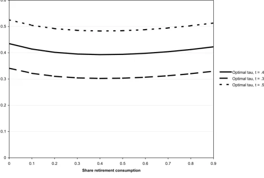
Expression (53) contains three share parameters: α, ω, and ¯γ. The share of observable costs in total educational expenditure is set at α = 0.5. Becker (1964) and Boskin (1975) find that the share of goods invested in education is about one-quarter and the share of (tax deductible) forgone earnings amounts to three-quarters. We do not set α to 0.75, however, because this would ignore the effort cost of education (i.e., attending college, studying, etc). The share of retirement consumption in total consumption is set at ω = 0.33. Finally, to compute ¯γ, we adopt an average ratio of lump-sum transfers to gross labor incomes of
g/z = 0.25.
As regards the three relevant behavioral elasticities in (53) (i.e., σ,β, andρ), the largest empirical literature exists on the intertemporal elasticity of substitution in consumption σ. Whereas older papers found extremely small elasticities, more recent work (e.g., Hall (1988) and Attanasio and Weber (1995)) suggests that the intertemporal substitution elasticity is substantially positive at around σ = 0.5.20 Trostel (1993) contains an extensive discussion
on plausible parameter values for the returns to inputs invested in human capital β. Based on this, we set β = 0.5.21 Concerning the elasticity of substitution between inputs in the
18The exogenously given revenue requirement Λ balances the budget.
19Estimated Mincer returns on education typically exceed 6%, see e.g. Ashenfelter et al. (1999). In
analogy of the equity premium puzzle, this raises the so-called human capital risk premium puzzle, see Judd (2000).
20This value may be on the high side for a three-period model with periods of about 20 years in which
intraperiod intertemporal substitution is in effect infinite. A lower value forσwould strengthen the case for large capital taxes further.
21The second-order conditions for individual utility maximization implyβ(1 +²n)<1.With the
compen-sated wage elasticity of labor supply²n taking an empirically plausible value of 0.5, βshould be smaller than
human capital formationρ, we follow Trostel (1993) by using ρ= 1 as the benchmark value. Hence, the production function if aggregate learning is Cobb-Douglas.
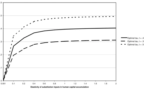
Figure 1 shows the optimal capital income taxes at given labor income taxes for the