NBER WORKING PAPER SERIES
HOUSING EXTERNALITIES Esteban Rossi-Hansberg
Pierre-Daniel Sarte Raymond Owens III Working Paper 14369
http://www.nber.org/papers/w14369
NATIONAL BUREAU OF ECONOMIC RESEARCH 1050 Massachusetts Avenue
Cambridge, MA 02138 September 2008
We thank Miklos Koren, Dan Tatar, and David Sacks for many helpful discussions. We also thank Marco Gonzales-Navarro, Gilles Duranton, and seminar participants at Yonsei University for their comments. Finally, we thank Brian Minton and Kevin Bryan for outstanding research assistance. The views expressed herein are those of the author(s) and do not necessarily reflect the views of the National Bureau of Economic Research.
NBER working papers are circulated for discussion and comment purposes. They have not been peer-reviewed or been subject to the review by the NBER Board of Directors that accompanies official NBER publications.
© 2008 by Esteban Rossi-Hansberg, Pierre-Daniel Sarte, and Raymond Owens III. All rights reserved. Short sections of text, not to exceed two paragraphs, may be quoted without explicit permission provided that full credit, including © notice, is given to the source.
Housing Externalities
Esteban Rossi-Hansberg, Pierre-Daniel Sarte, and Raymond Owens III NBER Working Paper No. 14369
September 2008
JEL No. D62,H23,R21,R31
ABSTRACT
Using data compiled from concentrated residential urban revitalization programs implemented in Richmond, VA, between 1999 and 2004, we study residential externalities. Specifically, we provide evidence that in neighborhoods targeted by the programs, sites that did not directly benefit from capital improvements nevertheless experienced considerable increases in land value relative to similar sites in a control neighborhood. Within the targeted neighborhoods, increases in land value are consistent with externalities that fall exponentially with distance. In particular, we estimate that housing externalities decrease by half approximately every 990 feet. On average, land prices in neighborhoods targeted for revitalization rose by 2 to 5 percent at an annual rate above those in the control neighborhood. These increases translate into land value gains of between $2 and $6 per dollar invested in the program over a six-year period. We provide a simple theory that helps us interpret and estimate these effects.
Esteban Rossi-Hansberg Princeton University Department of Economics Fisher Hall Princeton, NJ 08544-1021 and NBER [email protected] Pierre-Daniel Sarte Research Department.
Federal Reserve Bank of Richmond PO Box 27622
Richmond, VA 23261 [email protected]
Raymond Owens III Research Department.
Federal Reserve Bank of Richmond PO Box 27622
Richmond, VA 23261 [email protected]
1
Introduction
The existence of cities is a manifestation of the presence of agglomeration forces between economic agents. While much has been written about the nature and characteristics of these forces, most studies have focused on agglomeration forces between producers. As a result, virtually all urban theories have these producer-based agglomeration economies at their core.1 In fact, agglomeration e¤ects can also result from interactions between residents. Speci…cally, they can take the form of housing externalities whereby improvements made to a particular house can have an e¤ect on the value of nearby houses. To the extent that these e¤ects decline with distance, this form of externalities can lead to the agglomeration of residents and, potentially, the formation of cities. Moreover, because the presence of housing externalities may justify government intervention, in that equilibrium allocations will di¤er from e¢ cient outcomes, assessing the importance of these externalities in practice is central to urban policy. In this paper, therefore, we study the magnitude and characteristics of housing externalities. We are interested in the e¤ects of housing externalities on average land prices and in how fast these e¤ects decline with distance. These are the key characteristics that lead to agglomeration.
The standard problem in measuring agglomeration e¤ects lies in the circular causation present in all spatial concentrations of economic activity. People and …rms locate in a spe-ci…c area because that area is particularly productive or pleasant to live in, but the area is particularly productive or pleasant to live in because others chose to reside or work at that location. This implies that identifying agglomeration e¤ects in the data requires an exogenous source of variation in the “attractiveness” of a given location. In this paper, we exploit such a source of variation by taking advantage of an urban revitalization program implemented in Richmond, Virginia, between 1999 and 2004: the Neighborhoods-in-Bloom (NiB) program. We describe the program and its associated policies in detail in Section 2. For now, we note that this program represented federally funded housing investments concentrated in a few disadvantaged neighborhoods. We know the location of homes that obtained direct funding, and the amount that was received. We also have information on housing prices and a comprehensive list of housing characteristics before and after the pro-gram was implemented. This information allows us, using a hedonic regression, to estimate land prices before and after the policy was implemented. Taking into account city-wide time e¤ects, we can calculate the e¤ects of the program in the various treated neighborhoods. Put another way, we estimate the e¤ects of the policy on land values controlling for investments 1See the theoretical survey in Duranton and Puga (2004) and the empirical survey in Rosenthal and
in observable housing characteristics. By carrying out this exercise only for houses that were not directly targeted by the Neighborhoods-in-Bloom program, we ensure that the e¤ects we measure are not the valuation of unobservable investments directly associated with its policies.
We estimate changes in land prices, following the Neighborhoods-in-Bloom program, that are consistent with the predictions of a simple theory of housing externalities. We present this theory in Section 3. In particular, increases in the returns to land decline with distance from the impact area. This e¤ect, which we measure nonparametrically in the data, emerges clearly and corresponds to housing externalities that decline by half approximately every
990 feet. The theory also has predictions for the magnitude of the e¤ects induced by the Neighborhoods-in-Bloom policies that are consistent with our measurements. Finally, we use the …ndings from our estimation exercise to obtain parameter values for our model. This step potentially allows the model to guide the design of urban policies, although we leave this task to future research.
The exercise we have just described does not directly allow us to make statements re-garding the total return to land associated with the Neighborhood-in-Bloom program. We are able to assess whether changes in land prices are consistent with housing externalities that decline with distance, and how fast they decline, but additional information is needed to draw conclusions regarding the average increase in land values associated with these external e¤ects. We use time e¤ects at the city level to control for any city-wide changes and, po-tentially, general equilibrium e¤ects induced by the Neighborhood-in-Bloom policies. That said, as indicated in Section 2, the magnitudes of these policies are generally small enough that they are unlikely to a¤ect land rents in the city as a whole. In order to identify the e¤ects of the revitalization policies that arise by way of housing externalities, one needs to take a stand on the scope of these externalities, and measure increases in land values over and above those at the boundary of a selected neighborhood. This is, in principle, problem-atic since we have little information regarding the scope of housing externalities, nor do we know whether other non-observables might have a¤ected land values at the boundaries of the neighborhoods under consideration. Fortunately, a key feature of Neighborhoods-in-Bloom o¤ers us an alternative approach.
One of the unique aspects of the study we carry out in this paper relates to the presence of a neighborhood that shares almost identical physical and demographic characteristics as those selected for urban revitalization. Although initially considered by the Neighborhoods-in-Bloom task force, this neighborhood did not ultimately receive funding for reasons that were secondary and non-economic in nature. Hence, we use it as a control with which to contrast our …ndings for neighborhoods explicitly targeted by the urban renewal program.
Two key results emerge: i) in contrast to the treated neighborhoods, our estimates of changes in land rents in the control neighborhood do not fall with distance as we move away from its centroid. This result is consistent with the idea that one cannot measure changes in land valuations resulting from housing externalities in the absence of an exogenous source of vari-ation in land prices, ii) we compute average land price increases in the control neighborhood and show that they fall signi…cantly short of those measured in the targeted neighborhoods. We then use the …ndings associated with the control neighborhood to infer increases in land values arising from externalities induced by the revitalization policies. We …nd land value gains in the targeted neighborhoods that range between $2 and $6 per dollar invested in the program over a six-year period.
To the best of our knowledge, there have been only few studies of housing externalities that rely on a policy experiment with individual housing transaction data, and none where the experiment was spatially concentrated to the degree of Neighborhoods-in-Bloom. In Section 5, we compare our …ndings with other work that exploit parametric approaches to measure the decline in externalities across space. In general, we …nd housing externalities that decrease somewhat slower with distance. Ioannides (2002) …nds important residential neighborhood e¤ects using neighborhood clusters in U.S. cities. These neighborhood e¤ects, which have received some theoretical and empirical attention in the literature, are broader than the housing externalities considered in this paper as they include other forms of social interactions. See for example Benabou (1996) for an insightful theoretical model describing these types of social interactions and their e¤ects. There are several studies, both theoretical and empirical, that have analyzed urban renewal projects. Davis and Whinston (1961), Rothenberg (1967), and Schall (1976) are notable early examples. None, however, include the type of detailed empirical work we perform in this paper. On a theoretical level, Strange (1992) provides an informative discussion of policy in the presence of strong interactions across neighborhoods.2
The rest of the paper is organized as follows. Section 2 describes the Neighborhoods-in-Bloom program. Section 3 presents the model and the e¤ects of housing subsidies on equilibrium outcomes. Section 4 discusses our empirical methodology and Section 5 presents our …ndings. Section 6 o¤ers concluding remarks.
2
The Neighborhoods-in-Bloom Urban Revitalization
Program
The Neighborhoods-in-Bloom (NiB) program was an outgrowth of the observation by Rich-mond city o¢ cials that during the previous 25 years, investment programs undertaken to revitalize areas within the city had demonstrated only limited success. They noted that the programs had often improved small areas–such as a city block–but in many instances, measurable improvement in the surrounding neighborhoods remained elusive.
In evaluating the features of previous programs, o¢ cials noted that investment activity— in most cases using federal funding sources–had often been targeted in a scattered fashion. This approach had the advantage of reaching a large number of city neighborhoods that quali…ed under federal guidelines, but available funding per area was necessarily limited. The resulting constraints on investment activity led to impacts on home prices in surrounding areas that were di¢ cult to gauge. Because city o¢ cials’ objective was to visibly raise the values of surrounding homes, an idea developed that investment concentrated in fewer areas might yield more measurable e¤ects. This approach, they reasoned, might lead to a more noticeable revitalization of the city’s housing stock than had the previous, more scattered approach.
To carry out this experiment, city o¢ cials began to identify potential areas for invest-ment, determine the number of sites to target and source funding. As had historically been the case, the City of Richmond had numerous areas that quali…ed for revitalization funding through the Department of Housing and Development’s (HUD) Community Development Block Grant (CDBG) and Home Investment Partnership (HOME) programs. Additional funding was made available through other federal monies as well as through the non pro…t Lo-cal Initiatives Support Corporation (LISC), a community development corporation (CDC). The CDBG and HOME funding was attractive to the city, in part, because it was outside money. Simply put, these funds come from the federal government, and the resulting in-vestments bene…t the city without reducing local spending on consumption or investment that would otherwise occur if the funds were raised through local taxes. Interestingly, LISC funding also has this advantage. Founded by the Ford Foundation, LISC is a national or-ganization headquartered in New York and is funded by nationwide donations. Because of this structure, funds that ‡ow from the organization to Richmond are e¤ectively exogenous as well in that they do not necessarily originate from local sources.
The selection process of investment sites was a multiple step process. Past scattered approaches to investment had been driven in part by political pressures to fund areas within nearly all city council members’districts. Aware that a more concentrated approach would
likely fund fewer sites than the number of districts, broad support of a small number of sites was a primary objective. To achieve that support, in mid 1998, Richmond administrators es-tablished an internal planning task force composed of the acting city manager, the assistant city manager, and representatives from a variety of city departments associated with hous-ing and economic development. Several members within the group developed indicators of neighborhood conditions and data that served as comparative portraits of the neighborhoods that quali…ed to receive CDBG or HOME funds. Throughout 1998 and into early 1999, sta¤ from the city’s Community Development Department met with community groups to explain and gather feedback on the approach. In particular, city sta¤ and members of the groups also toured the potential sites, and support for both the concept and for a small group of neighborhoods had come together by February 1999. Later that year, the city community development department recommended four broad neighborhoods. These were Church Hill Central, Southern Barton Heights-Highland Park-Southern Tip, Jackson Ward-Carver, and Blackwell. The locations and size of these neighborhoods relative to the city of Richmond are shown in Figure 1.
Table 1A.Demographics of selected neighborhoods
Total Housing Percent Percent
Neighborhood Persons Units Non-White Below Poverty
Church Hill 1505 822 94.8 27.2 Blackwell 1376 651 97.0 35.8 Highland Park-Barton 2763 1227 97.2 26.3 Jackson Ward-Carver 1975 1332 81.7 29.5 Bellemeade 2742 947 90.2 31.6 City of Richmond 197790 92282 61.5 20.3
These four neighborhoods share many common characteristics. All had been selected according to criteria developed by the city’s community development sta¤ and had con-centrations of vacant structures, substantial poverty, and low home ownership rates. In addition, the capacity of the areas to revitalize absent NiB investment was viewed as low. The neighborhoods also had active nonpro…t Community Development Corporations (CDCs) in place. This was an important feature in that funds from the HUD programs are generally disbursed through these organizations which perform new home construction, rehabilitation, and renovations that comprise the vast majority of investment activity in the neighborhoods. Although the selected NiB neighborhoods share many similarities, one important distinction must be made in that Blackwell was subject to an additional urban program, known as HOPE VI, alongside NiB. HOPE VI was a program designed to raze un…t homes, without at
the time creating new construction in their place. Tables 1A and 1B provide a summary of basic demographic and housing characteristics of the selected neighborhoods using the 2000 census and our housing data before the start of the program in 1998.
Table 1B. Characteristics of the housing stock in NiB neighborhoods Percent Percent Average Median Price
Neighborhood Vacant Owned Plot Acreage Pricea St. Dev.
Church Hill 21.7 35.7 0.07 14,861 29,244 Blackwell 23.2 32.6 0.09 17,368 16,705 Highland Park-Barton 18.3 40.5 0.14 33,223 24,740 Jackson Ward-Carver 31.5 36.0 0.06 37,914 46,548 Bellemeade 10.8 51.4 0.16 33,881 15,643 City of Richmond 8.4 46.1 0.17 74,394 121,539
a :expressed in 2000 constant dollars
As shown in Figure 1, the selected neighborhoods all fall in the eastern part of the city and share a heritage dating to Richmond’s origins. The city was founded because of its location at the fall line of the James River, the farthest inland point navigable to ship tra¢ c. Early development began in this area, but as factories emerged, the neighborhoods in the eastern portion of the city gradually fell into disfavor and declined over time. This process led to changes in the demographic makeup of these areas, with higher poverty rates and lower average home prices, as well as higher percentages of crime relative to citywide averages. Aside from their similarities in terms of demographics, homes in the selected neighborhoods, because of their historical ties, also share many elements of style and construction. In particular, homes in all selected areas consist mostly of row houses of similar sizes, many constructed of brick. A slight exception is Blackwell and Highland Park, where some homes are of detached Queen Anne and Victorian styles.
With funding sources in place and neighborhoods identi…ed, NiB began operations in July 1999. Prior to start up, teams were formed comprised of city sta¤ers, community group representatives, and CDC representatives to review neighborhood redevelopment plans, iden-tify precise boundaries of investment, known as “impact areas”, and ideniden-tify speci…c homes for renovation and sites for new home construction. Once speci…c home projects within individual impact areas were determined, the CDCs operating in those areas applied for funds to carry out the projects. Nearly all investment activity consisted of acquisition, de-molition, rehabilitation, and new construction of housing within NiB impact areas. The work carried out by the various CDCs varied in impact, re‡ecting in part the comparative
strengths of individual organizations, in that speci…c CDCs had unique relationships with their home neighborhoods and specialized experience in some categories of construction or rehabilitation.
Spending under the NiB program began in 1999 (although a small fraction preceded the o¢ cial start date of the program) and continued through 2004. Over this period, approxi-mately $14 million was spent in total. Slightly over $11 million came through CDBG and HOME programs, smaller federal programs and Commonwealth of Virginia monies. LISC added nearly $3 million. Around $1 million came from other sources, with approximately half that amount from undocumented sources. Most of the spending took place in the 1999 through 2001 period, with yearly expenditures trailing o¤ in the later years of the program. Finally, one of the unique aspects of the study we carry out in this paper relates to the presence of a neighborhood that was almost included in the NiB program but that did not, ultimately, received funding. Speci…cally, the neighborhood of Bellemeade lies in the eastern portion of the city, south of the James River (see Figure 1). Its makeup and location are typical of NiB neighborhoods and, according to a former city o¢ cial closely involved with the NiB selection process, “absolutely matched”the selected neighborhoods in physical and demographic terms. This is in fact also clear from Tables 1A and 1B. The reason that Bellemeade did not make the …nal cut, he suggests, is that the area did not have active enough CDCs, so that the channel used to direct NiB investment dollars was mostly absent. This distinction, however, makes Bellemeade close to an ideal control neighborhood. In particular, because no NiB investment took place in that neighborhood, and given that its demographics and housings stock closely match that of the selected NiB neighborhoods, it is natural to use Bellemeade as a benchmark in gauging changes in neighborhood land values arising from the NiB program.3
3
A Model of Housing Externalities
This section provides a framework that o¤ers insight into the types of urban renewal policies we have just described. More importantly, it helps underscore the importance of housing ex-ternalities in determining the e¤ects of these revitalization policies. Consider a neighborhood represented byN = [ R; R], whereR denotes the neighborhood’s edge, with density of land 3A question remains as to why there were fewer CDC’s in Bellemeade than in the other neighborhoods
in the …rst place, which potentially indicates a lingering selection issue. The results presented in Section 5, however, suggest that this concern is limited.
equal to one. All agents living in the neighborhood work at location0.4 We assume that all agents are endowed with one unit of time, and that some of this time is spent commuting to work. Thus, an agent commuting from location ` 2 N only works e j`j time units, >0. The production technology is linear, and transforms one unit of time intow units of a …nal good.
Agents’preferences are de…ned over housing services enjoyed at a given location, denoted byHe(`)for an agent living at`, and other types of consumption,c(`). The only good in the economy can be allocated to either investment in housing or consumption. All agents live on a lot of size one, which they rent from absentee landlords at rateq(`). Housing services at a location are obtained from owning a piece of land and directly improving it, as well as from the amount of housing services produced nearby. The fact that housing services produced at a given location a¤ect housing services enjoyed elsewhere de…nes a housing externality. Formally, if H(`) denotes investments in housing undertaken by an individual living at `, then e H(`) = Z R R e j` sjH(s)ds+H(`): (1)
Hence, aside from home improvements they make at a given location, individuals also bene…t from having nearby housing owned by others that is well-maintained. In particular, housing services enjoyed at location` re‡ect in part a weighted average of housing services produced at neighboring sites, with weights that decline with distance at an exponential rate >0.
Agents living at location ` spend their income, we j`j, on the unit of land they rent at
rate q(`), housing investments, H(`), and consumption, c(`). We assume that individuals order consumption baskets according to a Cobb-Douglas utility function. Hence, an agent living at some location ` solves
max c(`); H(`)u(c(`); e H(`)) = c(`) He(`)1 ; 0< <1; (P`) subject to c(`) +q(`) +H(`) =we j`j; (2) and e H(`) = Z R R e j` sjH(s)ds+H(`);
where housing services produced at other locations,H(s), are taken as given. The optimality conditions associated with problem (P`) imply that
(1 )c(`) = He(`): (3)
4This simplifying assumption ensures symmetry but is otherwise unimportant for the questions we shall
Substituting this condition into the agent’s budget constraint (2), and using the equation describing the externality from housing (1), immediately yields an expression for housing services obtained at ` that depends only on prices and housing services produced elsewhere,
e
H(`) = (1 ) we j`j q(`) +
Z R R
e j` sjH(s)ds : (4)
3.1
The Neighborhood Equilibrium
There are two key conditions that determine equilibrium allocations in the neighborhood. First, all agents are identical and can choose freely where to live, including in another neighborhood if their utility falls below some reservation utility,u. In equilibrium, therefore, individuals obtain utility uat all locations, which immediately implies that
e
H(`) H =u 1 : (5)
That is, housing services enjoyed at any location are the same throughout the neighborhood. It follows from Equation (1) that the function describing housing investments at di¤erent sites is a …xed point of the following functional equation,
H(`) = H
Z R R
e j` sjH(s)ds; `2[ R; R]: (6)
The second condition needed to determine equilibrium allocations involves a boundary con-dition for land rents at either edge of the neighborhood, which we denote by qR >0. From
equations (4) and (5), land rents in the neighborhood are given by
q(`) = we j`j+
Z R R
e j` sjH(s)ds 1
1 H: (7)
At the boundary, therefore, we have that R implicitly solves
Z R R
e j` sjH(s)ds= 1
1 H+qR we
R. (8)
To summarize, an equilibrium for the neighborhood is a function describing housing invest-ments at all locations,H(`), a function describing land rents, q(`), a level of housing services
H, and a boundary for the neighborhood, R, such that equations (5), (6), (7) and (8) are satis…ed.
The solid curves in Figure 2A and 2B depict typical equilibrium housing investment al-locations, H(`), and land rents, q(`), respectively.5 Housing investments are highest near 5The parameter values used in this example are: u= 13:25, = 0:001, R= 3500,A= 1190, = 0:368,
the boundaries of the neighborhood where externalities from housing are lowest. With lower externalities from housing at locations away from the neighborhood center, individuals living at those locations must spend a greater share of their income on direct home improvements in order to obtain the constant level of housing servicesH. The fact that housing externalities are lowest near the neighborhood boundaries also implies that land rents are lowest at those locations. On a more practical level, observe in Figure 1 that the highlighted neighborhoods are indeed often bounded by major roads, such as interstates or highways, and other land-marks that e¤ectively reduce externalities from housing potentially located outside those boundaries. The neighborhood of Blackwell, for instance, is bounded by highways to the west, north, and east, as well as by an industrial railway station in part to the south. Simi-larly, the neighborhood of Jackson Ward-Carver is bounded by Interstate 64 to the north and Highway 250 to the south, and adjoins an industrial zone to the east. Although not bounded by main roads, the land surrounding Highland Park-South Barton Heights is largely free of housing, composed of a large cemetery to the south, warehouses to the west, and vacant grounds to the east and north.
3.2
The Neighborhoods-in-Bloom Program
Consider a federally funded neighborhood revitalization program that aims to increase hous-ing investments at all locations in an area A = [ r; r] N by some …xed amount > 0. Throughout the paper, we refer toA as an ‘impact area.’ LetHp(`)denote the new
equilib-rium housing investment function that emerges after implementation of the policy. Similarly, letHep(`)describe housing services enjoyed at location` following the program. Because the
reservation utility from living in some other neighborhood is unchanged, and agents can freely move between neighborhoods, housing services are still given by Equation (5) so that
e
Hp(`) =H. Then, for` 2 N nA, Hp(`) solves
H=Hp(`) + Z R R e j` sjHp(s)ds+ Z r r e j` sjds; (9)
where the last term in (9) captures externalities generated by the program and obtained at a location outside the impact area. For locations ` 2 A that are directly a¤ected by the revitalization policy, we have that
H =Hp(`) + Z R R e j` sjHp(s)ds+ Z r r e j` sjds+ 1 ; (10)
where the last term now re‡ects the fact that those locations are also the direct recipients of capital improvements .
Since H remains unchanged following the urban development program, it follows that
H(`)p H(`) < 0 for all ` 2 [ R; R]. To see this, note from equations (6) and (9), and
abstracting from the direct subsidy, that for `2 N nA,
H(`)p H(`) = Z R R e j` sj[Hp(s) H(s)]ds Z r r e j` sjds = Z r r e j` sjds+ Z R R e j` jj Z r r e jj sjdsdj 2 Z R R e j` jj Z R R e jj kj Z r r e jk sjdsdkdj+::: < 0 (11) since Z R R e j` sjds= Z 2R 0 e sds = e s 2R 0 = 1 e 2R <1;
so that Rrre jj sjds < 1 as well. The direct e¤ect of subsidies, of course, only serves
to amplify this e¤ect in the impact area. Put another way, Equation (11) implies that investment in housing decreases everywhere in the neighborhood, and this decrease is more pronounced the closer the locations are to the impact area. In this framework, therefore, the neighborhood revitalization program crowds out private investment in housing. The subsidy to home improvements in e¤ect allows agents to enjoy housing services without having to spend on those services themselves. The implied relaxation of their budget constraint leads individuals to bid up the price of land so that, in the new equilibrium, higher land rents,
qp(`), prevail throughout the neighborhood.
The di¤erence in land rents created by the implementation of the policy, net of the direct capital improvement , is given by
qp(`) q(`) = Z R R e j` sj[Hp(s) H(s)]ds+ Z r r e j` sjds >0: (12)
We have already argued that the …rst term in square brackets is negative. The second term captures positive externalities generated by the capital improvement policy. In this respect, the size of the exogenous increase in housing investment at each targeted location, , and the extent of the impact area, A, have a …rst order positive e¤ect on land prices. In contrast, because commuting costs, , and income, w, a¤ect land rents in the same way in (7), both before and after the introduction of the policy, these features are essentially di¤erenced out and only a¤ect land prices through changes in H(:) in Equation (12). Note that sinceqp(`) q(`)in (12) is simply the negative of the change in land rentsHp(`) H(`)
in (11), it immediately follows that qp(`) q(`) > 0. Hence, our assumption of
H following the policy) ensures that the implementation of the revitalization program is associated with higher land rents. This choice of preferences stems from empirical work on cities which has found the Cobb-Douglas speci…cation with respect to land and consumption to …t the data well (see Davis and Ortalo-Magne, 2007).
In the end, as a result of the revitalization program, housing investments fall and land prices rise throughout the neighborhood. Agents consume a constant fraction of housing, and now that nearby homes o¤er additional housing services, they prefer to invest less where they live. The revitalization policy increases the value of location and, therefore, land prices. We summarize these results in the following proposition:
Proposition 1 Following the positive housing subsidy on a set of locations A, housing in-vestments decrease at all locations, H(`)p H(`) < 0 8` 2 [ R; R], and land rents
increase at all locations, qp(`) q(`)>0 8`2[ R; R].
The new equilibrium land rents,qp(`), are described by the dashed curve in Figure 2B. As
we have just argued, these new land rents are everywhere higher in the neighborhood, and especially when close to the impact area. Figure 2C shows the percentage or log di¤erence between post-policy and pre-policy land rents on either side of the center of the impact area, net of the direct capital improvements brought about by the renewal program. This di¤er-ence, therefore, re‡ects only the propagation of housing externalities across space induced by the federal housing investment increase.
Given that externalities fall exponentially with distance in this model, increases in land value in Figure 2C will generally mimic a di¤usion process as they level out with distance from the impact area. The rise in land rents is more pronounced over the impact area because a typical location in that area is mainly surrounded by other locations that received funding for capital improvements. Hence, a location inA bene…ts from externalities generated by many similarly a¤ected locations nearby. Note, in particular, the steep drop o¤ in land returns once we move outside the impact region. At locations near the boundary, di¤erences in land rents become mostly ‡at near zero in Figure 2C. This e¤ect arises because any one location near the boundary, contrary to a location inA, is mainly surrounded by other locations that did not bene…t from the revitalization program. External e¤ects from the policy, therefore, are negligible at those locations. Because externalities generate a two-tier e¤ect on land rents across space, changes in land rents produced by the revitalization program will generally be characterized by a bimodal distribution. This is shown in Figure 2D. Keep in mind, from Equation (12), that this bimodal aspect of land returns arises independently of the direct e¤ect related to capital improvements in A.
4
The Empirical Framework
This section sets up an empirical framework whose aim is to help us identify the extent to which the e¤ects of the NiB programs, in practice, propagated to non-targeted sites. We are also interested in whether we can establish empirically that these external e¤ects decline with distance in a way suggested by Figure 2C. If so, we also wish to a gauge how far the e¤ects of NiB programs were able to extend in this case.
We denote a location in the city of Richmond by ` = (x; y) 2 R2, where x and y are Cartesian coordinates. Let p represent the (log) price of a home per square foot of land in the city of Richmond. Our analysis begins with the following semiparametric hedonic price equation,
p=Z +q(`) +"; (13)
whereZ is a k element vector of conditioning housing attributes such thatcov(Zj`) = zj`,
q(`)is the component of home prices directly related to location, and" is a random variable such that E("j`;Z) = 0 and var("j`;Z) = 2
". While this semi-log speci…cation is standard
in the analysis of real estate data, we di¤er somewhat in that we try to remain ‡exible with respect to the form ofq(`). In particular, we do not assume thatq(`)lies in given parametric family.6
We are interested in assessing the e¤ects of NiB policies on the component of prices related to location, q(`), in the various targeted neighborhoods described previously. This suggests estimating Equation (13) both before and after the NiB policies come into e¤ect. Because our concern is with assessing the extent of residential externalities, we omit obser-vations on homes that directly bene…ted from NiB funding in our estimation. Although our model predicts that the types of renewal programs considered here generally crowd out of private investment, it is conceivable that these programs induced a reshu- ing of heteroge-nous populations across neighborhoods, consistent with gentri…cation, that is not captured in our framework. In particular, a higher income household that decided to relocate to an impact area and further invested in home improvements would have very likely used some NiB funding (since the program aimed to precisely subsidize this type of investment). As such, simply subtracting public home improvements at that location would overstate the external e¤ect of the policy on land prices. Because we have no way of measuring any ad-ditional private spending on home improvements at locations that received NiB funding, a 6The assumption of separability betweenZ andq(`)is made for computational simplicity, and abstracts
from a potential complementarity between location and housing attributes. See Ho (1995), and Anglin and Gencay (1996), for alternative applications of the semiparametric hedonic pricing model to the real estate market.
conservative strategy is to omit the observation altogether.
Some key questions that the analysis will attempt to uncover are: i) How did the price of land change in each of the neighborhoods in Figure 1, say fromq(`) toqp(`), at sites not
directly targeted by the NiB revitalization projects? ii) Can we relate this change to some notion of distance from a focal point in a given impact area? In particular, do the …ndings related to the neighborhoods targeted for revitalization indicate external e¤ects that dissipate with distance? Conversely, given the absence of an impact area in the control neighborhood of Bellemeade, are land price changes in that neighborhood more uniform across space?
4.1
Data Description
Our dataset stems from two sources. First, the city of Richmond collected records of all properties that bene…ted from NiB funding between 1999 and 2004. These records include the geo-coded location of those properties as well as the amount and type of funds that it re-ceived. Second, we also obtain from the city of Richmond a geo-coded listing of all properties sold between1993and2004that includes information on condition and age, construction de-scriptors (e.g. exterior materials, type of heating, etc.), and various dimensional attributes (e.g. lot size, size of living area, etc.). Since the NiB revitalization programs speci…cally targeted residential properties, we remove from our sample all non-residential properties, mainly commercial buildings. We also delete listings that were likely incorrectly recorded, including homes listed as being built before 1800 and homes whose living area is recorded as less than250 square feet. Because all of our data is geo-coded, we are able to cross-check our two datasets and remove any property that directly bene…ted from NiB funding. In this sense, we aim to measure only the external e¤ects associated with the NiB programs. In all, we have44;412 sales observations.
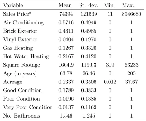
Descriptive statistics of the housing characteristics for all years are reported in Table 2. These characteristics include the furnished square footage of a house, the number of years since the house was …rst built, its plot acreage, and the number of bathrooms available (with half baths counting as one half). We also include binary variables that indicate whether the house has central air conditioning, whether its exterior is brick or vinyl, and whether it is heated using gas or hot water. The city of Richmond also assigns condition grades to each house, which we capture using binary variables to indicate whether a house was assessed in good condition, poor condition, or very poor condition. Finally, we include among our conditioning variables, Z, a set of time dummies that capture secular city-wide increases in home prices driven by aggregate factors such as city population growth or interest rates changes.
Table 2. Data Summary
Variable Mean St. dev. Min. Max.
Sales Pricea 74394 121539 11 8946680
Air Conditioning 0.5716 0.4949 0 1 Brick Exterior 0.4611 0.4985 0 1 Vinyl Exterior 0.0404 0.1970 0 1
Gas Heating 0.1267 0.3326 0 1
Hot Water Heating 0.2167 0.4120 0 1 Square Footage 1664.9 1190.3 319 63233
Age (in years) 63.78 26.46 0 205
Acreage 0.2337 0.3506 0.012 37.67
Good Condition 0.1789 0.3833 0 1 Poor Condition 0.0196 0.1385 0 1 Very Poor Condition 0.0137 0.1162 0 1
No. Bathrooms 1.546 1.245 0 1
a:Expressed in constant 2000dollars.
4.2
Estimation of the Parametric E¤ects
In order to estimate the non-parametric component of Equation (13), q(`), we must …rst address the estimation of the parametric e¤ects, . Letn denote the number of observations on home prices and k the number of variables in Z. A popular approach, pioneered by Robinson (1988), proceeds in two steps. In the …rst step, non-parametric (kernel) estimates of E(pj`) and E(Zj`) are constructed. Since Equation (13) implies that
p E(pj`) = [Z E(Zj`)] +"; (14)
the second step involves replacing the conditional means in (14) by these non-parametric functions and estimating by least squares. Robinson (1988) shows that estimates of obtained in this way are pn consistent. Because of the size of our dataset, and given that separate non-parametric regressions are required for each housing attribute inZ, this method proves onerous in our case. To circumvent this problem, Yatchew (1997, 2001) proposes a di¤erencing approach that we adopt in this paper.
The basic idea behind Yatchew’s (1997, 2001) estimation strategy is to re-order the data,
(p1;Z1; `1), (p2;Z2; `2), ... , (pn;Zn; `n) so that the `’s are close, in which case di¤erencing
tends to remove the non-parametric e¤ects. In particular, …rst-di¤erencing of (13) gives
Assuming that a Lipschitz condition holds forq,jq(`a) q(`b)j Ljj`a `bjj, the di¤erence in
non-parametric component in (15) vanishes asymptotically.7 Yatchew (1997) shows that the OLS estimator of using the di¤erenced data (i.e. the projection ofpi pi 1onZi Zi 1) is alsopn consistent. This estimator of , however, achieves only2=3e¢ ciency relative to the one produced by Robinson’s method. This can be improved dramatically by way of higher-order di¤erencing. Speci…cally, de…ne p to be the (n m) 1 vector whose elements are
[ p]i =Pms=0dspi s, Zto be the(n m) k matrix with entries [ Z]ij = Pm
s=0dsZi s;j, and similarly for ". Theds’s denote constant di¤erencing weights andm governs the order
of di¤erencing. We thus estimate a more general version of Equation (15),
p= Z +
m X s=0
dsq(`i s) + "; i=m+ 1; :::; n; (16)
where the following two conditions are imposed on the di¤erencing coe¢ cients, d0; :::; dm : m X s=0 ds= 0 and m X s=0 d2s = 1: (17)
The …rst condition ensures that di¤erencing removes the non-parametric e¤ect in (13) as the sample size increases and the re-ordered `’s become “close”. The second condition is a normalization restriction that implies that the transformed residual in (16) has variance 2".
When the di¤erencing weights are chosen optimally, the di¤erence estimator, , obtained by regressing p on Z approaches asymptotic e¢ ciency by selectingm su¢ ciently large.8 We use m = 10 which produces coe¢ cient estimates that are approximately 95percent e¢ cient when using optimal di¤erencing weights. Note that, as a practical matter, the initial re-ordering of the `’s is not unambiguous here since ` 2 R2. We re-order locations using a path created by a Hamiltonian nearest neighbor algorithm and, for our dataset, this yields a mean distance between locations, 1=nPjj`i `i 1j, that is 24 to 28 times smaller than that obtained by simply re-ordering locations according to their x or y coordinate (i.e. the wrap-around method)9.
7Suppose that locations constitute a uniform grid on the unit square (the re-scaling is without loss of
generality). Each point may then be thought of as residing in an area of 1=n, and the distance between re-odered adjacent observations,jj`i `i 1jj, is1=pn.
8Optimal di¤erencing weights,d
0; :::; dm, solvemin =Pmk=1(
P
sdsds+k)2subject to the constraints in
(17). See Yatchew (1997).
9The starting point when using the nearest neighbor approach is arbitrary but has little implications for
4.3
Non-Parametric Kernel Estimation of
q
(
`
)
Denote by Y the price of a home “purged” of its contribution from housing characteristics, whereY is obtained using …rst stage estimates,Y =p Zb , and construct the data(Y1; `1),
(Y2; `2),...,(Yn; `n). Because b is a consistent estimator of , standard kernel estimation
methods applied to purged home prices yield consistent estimates of q(`). The Nadaraya-Watson kernel estimator of q at location`j is given by
q(`j) = n 1 n X
i=1
Whi(`j)Yi. (18)
In other words, the component of home prices directly related to location, `j, is a
weighted-average of the Y’s in our data sample. The weightWhi(`j)attached to each priceYi is given
by Whi(`j) = Kh(`j `i) n 1Pn i=1Kh(`j `i) ; (19) where Kh(u) =h 1K( u h);
and K( ) is a symmetric real function such that R jK( )jd < 1 and R K( )d = 1. Thus, we may choose to attach greater weight to observations on prices of homes located near `j rather than far away by suitable choice of the functionK. In particular, as in much
of the literature, our estimation is carried out using the Epanechnikov kernel. The distance between location`j and some other location`i in the city is simply measured as a Euclidean
distance in feet. An implication of the Epanechnikov kernel is that prices of homes located more than a distance of h feet from `j will receive a zero weight in the estimation of q(`j).
In that sense, the bandwidth h has a very natural interpretation in this case.10
The NiB programs were …rst implemented in 1999 and nearly phased out by 2004. Con-sequently, we estimate Equation (13) over two subsamples, 1993 1998, the period prior to NiB coming into e¤ect, and 1999 2004, the post revitalization period for which we have data. The …rst and second subsamples contain 18102 and 26310 observations respectively. Ultimately, we wish to capture increases in the price of land at di¤erent locations between
1998 and 2004. Hence, we set the base year for the time dummies in Z as the last year in each subsample period. All prices are measured in 2000 constant dollars, and we estimate land prices using observations over the entire city of Richmond.
10In practice, the estimation ofq(`)is a¤ected to a greater degree by the choice of bandwidth rather than
the choice of kernel. See diNardo and Tobias (2001) for a detailed discussion. In this case, the bandwith is chosen by means of Cross-Validation. Hence, we select hso that it solves minhCV(h) = n 1Pnj=1[Yj
e
5
Empirical results
This section reviews our …ndings. We present estimates of the semiparametric hedonic price regression (13) and illustrate what they imply for city-wide land prices prior to the imple-mentation of NiB. This allows us to compute changes in land values for the neighborhoods targeted for revitalization and describe how these changes vary as we move away from the impact area. We then compare our …ndings for the targeted neighborhoods with those in our control neighborhood. This comparison lets us compute the total e¤ect of the NiB program relative to a benchmark where no such public investment took place. Finally, we use this evidence to calibrate the model of housing externalities presented in Section 3.
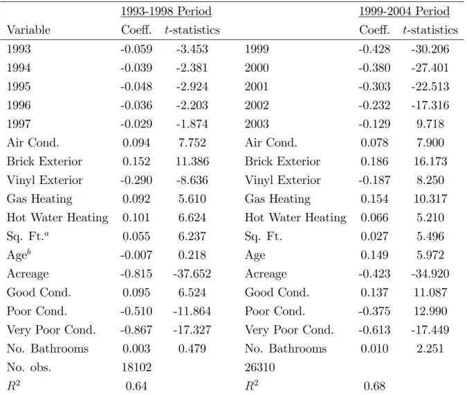
Table 3 presents estimates of the parametric components of Equation (13). Virtually all housing characteristics in Table 3 are statistically signi…cant at the 5 percent critical level, and the large majority of these attributes is signi…cant at the 1 percent level in both samples. In addition, both speci…cations achieve a surprisingly good …t for cross-sectional data.11
Coe¢ cients associated with the sale date are signi…cant over and above prices being measured in constant dollars. In the post 1998 period, in particular, our …ndings suggest a considerable real run up in home prices in the city of Richmond (as with many other U.S. cities over the same time period). We estimate separate semiparametric hedonic price speci…cations over the pre and post 1998 period to account for possible changes to the valuation of housing attributes triggered by the implementation of the revitalization policy or any other city policy or shock. The housing coe¢ cients shown in Table 1, however, tend to be relatively similar across subsamples. Alternative estimates that hold the coe¢ cients on housing attributes constant across subperiods have immaterial implications for the results we present below.
Of central interest are the nonparametric estimates of land prices, q(`), in both the targeted neighborhoods and the control neighborhood.12 Prior to the start of the NiB project, we estimate land prices that in1998 averaged $5.97 per square foot in the neighborhood of Church Hill, $6.38 in Highland Park-South Barton Heights, and $5.17 in Blackwell. In contrast, we estimate higher land prices for the city as a whole, with a mean of $8.29 per square foot, and land prices that are as high as $100 per square foot in the more a- uent parts of Richmond. The large majority of these highly priced sites form part of a historical district known as the Fan located in the center of Richmond. Because the neighborhood of Jackson Ward-Carver adjoins the Fan district, the local averaging implied by kernel estimation gives
11It can be shown thats2 = 1 n Pn i=1( pi Zib ) 2 !P 2 ". Hence, we computeR2 as1 s2=s2p.
12Land prices are estimated on a grid containing the coordinates of home sales in our pre-policy sample.
land prices that have a mean of $12 per square foot in that neighborhood. In contrast, estimated land prices in the control neighborhood of Bellemeade fall well within the range of the other three NiB neighborhoods, with a slightly lower mean at $4.71 per square foot.
Table 3. Estimates of the parametric e¤ects on home prices
1993-1998 Period 1999-2004 Period
Variable Coe¤. t-statistics Coe¤. t-statistics
1993 -0.059 -3.453 1999 -0.428 -30.206
1994 -0.039 -2.381 2000 -0.380 -27.401
1995 -0.048 -2.924 2001 -0.303 -22.513
1996 -0.036 -2.203 2002 -0.232 -17.316
1997 -0.029 -1.874 2003 -0.129 9.718
Air Cond. 0.094 7.752 Air Cond. 0.078 7.900
Brick Exterior 0.152 11.386 Brick Exterior 0.186 16.173 Vinyl Exterior -0.290 -8.636 Vinyl Exterior -0.187 8.250
Gas Heating 0.092 5.610 Gas Heating 0.154 10.317
Hot Water Heating 0.101 6.624 Hot Water Heating 0.066 5.210
Sq. Ft.a 0.055 6.237 Sq. Ft. 0.027 5.496
Ageb -0.007 0.218 Age 0.149 5.972
Acreage -0.815 -37.652 Acreage -0.423 -34.920
Good Cond. 0.095 6.524 Good Cond. 0.137 11.087
Poor Cond. -0.510 -11.864 Poor Cond. -0.375 12.990 Very Poor Cond. -0.867 -17.327 Very Poor Cond. -0.613 -17.449 No. Bathrooms 0.003 0.479 No. Bathrooms 0.010 2.251
No. obs. 18102 26310
R2 0.64 R2 0.68
a :measured in 1000sq. ft.; b :measured in 100 years.
A contour map of the price of land per square foot for the city of Richmond before NiB is shown in Figure 4. It is clear from the …gure that the NiB neighborhoods are associated with some of the lowest land prices in the entire city.13 Despite its relatively small area of60square miles, Figure 4 suggests considerable variation in land prices throughout Richmond. Because lot sizes are relatively homogenous throughout Richmond at around0:1acres, our estimates suggest lot prices that vary from $20,000 in the neighborhoods targeted by NiB to $435,000 in the more well-o¤ districts. Table 4 focuses on the NiB neighborhoods more speci…cally 13To capture policy e¤ects that potentially extend beyond the areas intially targed by NiB, we present our
and gives estimated land prices per square foot at di¤erent percentiles in comparison to the city as whole.
Table 4. Pre-NiB land price per square foot
10th 25th 50th 75th 90th
Neighborhood Percentile Percentile Percentile Percentile Percentile
Church Hill 0.81 1.84 5.21 13.32 21.02 Blackwell 0.76 1.84 3.83 7.04 12.15 Highland Park-Barton 1.29 2.61 5.22 8.05 11.59 Jackson Ward-Carver 2.22 4.85 11.77 21.66 31.36 Bellemeade 1.87 2.89 4.71 6.42 8.13 City of Richmond 3.09 5.11 8.29 14.94 27.40
5.1
The Return to Land in the Neighborhoods Targeted by NiB
To relate our empirical …ndings to the theory in Section 3 more closely, we now explore several key aspects of the data. First, we explore whether changes in land value in the four selected neighborhoods decrease with distance in a way suggested by Figure 2C? Second, given the absence of an impact area in the control neighborhood of Bellemeade, we ask whether changes in land value in that neighborhood are both lower and more uniform across space.To answer these questions, there are two aspects of the empirical framework that we must …rst reconcile with the theory presented in Section 3. First, in contrast to our model, targeted neighborhoods in practice generally have more than one impact area. Second, for ease of presentation, we must tackle the issue of how to present our estimates for q(`), where ` 2 R2, in terms of distance from a focal point, q(d), where d 2 R, analogously to Figure 2C. By way of example, we use the neighborhood of Blackwell to discuss our approach to both issues, and proceed similarly in the other targeted neighborhoods.
Figure 3 shows the targeted neighborhood of Blackwell, denoted by N. Within N, let Ai represent the cluster of locations that were the direct recipient of NiB funding. There are
2 such clusters shown in Figure 3, which essentially constitute impact areas. Formally, the partitioning of directly targeted locations into separate clusters satis…es aK-means criterion. Speci…cally, our partitioning of those locations into 2 disjoint subsets, A1 and A2, satis…es
respectively.14 We de…ne the funding center of an impact area as a convex combination of the locations that received NiB funding within that cluster. These are shown asc1 andc2 in Figure 3. The weights in that combination are given by the relative amounts of NiB funds spent at the di¤erent locations. In that sense, this funding center represents a focal point of the revitalization policy in a given impact area.
In general, it is possible that a location in between two impact areas, such as between A1 and A2 in Figure 3, bene…t from externalities related to both sets of funded locations simultaneously. In that case, for simplicity, we attribute any measured external e¤ect on land values to the closest impact area. Thus, for each location ` in N, we compute the distance from ` to the center of the closest cluster, d(`) = minifjj` cijjg, where ci is the center of
Ai. We can then rank these distances from smallest to largest. In particular, the variable
d(`) represents a convenient mapping from R2 to R that, despite the existence of several impact areas in a given neighborhood, captures some notion of distance from a central point of the policy experiment. It also allows us to plot land price changes with respect to distance from this focal point, q(d), and to examine whether changes in land value indeed fall as we move away from the policy experiment (i.e. asdincreases). In order to capture any external e¤ects that potentially exist beyond the targeted neighborhoods in Figure 1, we extend each neighborhood to encompass locations such that d(`) covers a radius of 3500 feet. In doing so, however, we are careful not to cross natural boundaries such as highways, railroad tracks, industrial zones, etc. that often arise before reaching 3500 feet. In practice, therefore, this radius generally represents the broadest de…nition of a neighborhood that does not infringe on other neighborhoods with distinctly di¤erent demographics or housing characteristics.
Figure 5 illustrates (kernel-smoothed) distributions of estimated land price changes,
q(`), in each of the NiB neighborhoods. Recall that q(`) is estimated from log prices so that q(`) measures percent changes which we express at an annual rate. The distribu-tion of estimated changes in land value generally depicts positive returns in all four cases, although the spread and mean of these distributions vary. The question is whether, as in Figure 2C, these land price increases become smaller as one moves further away from the impact area.
Figure 6 illustrates the behavior of estimated changes in land prices per square foot with respect to distance from the impact area, q(d). It is apparent that in all four cases, the returns to land fall as the distance from the policy experiment increases.15 Externalities 14Although this problem potentially yields multiple solutions, the clusters of funded locations are su¢
-ciently separated in our case that this is not an issue.
15The curves shown in each panel of Figure 6 are Nadaraya-Watson kernel estimates computed as described
are more pronounced close to the funding center and fall steeply as one moves away from locations in the impact area. In the neighborhood of Church Hill (Figure 6A), most of the returns to land are concentrated around the upper tier, which explains a mode annual return of around 12 percent in Figure 5A. In contrast, in the neighborhood of Blackwell (Figure 6B), most of the returns to land are located near the lower tier so that the mode return in Figure 5B is around 4:5percent. Both Figures 5 and 6 suggest perceivable di¤erences in the way that each neighborhood was a¤ected by the NiB program, with mean annualized returns that vary from 5:93percent in Blackwell to 9:71percent in Church Hill. Thus, we examine more closely below the relationship between the size of the capital improvement program in a particular neighborhood and its overall gain in value from externalities. Recall from Equation (12) that both the size of the impact area and the amount of funding for home improvements have a …rst-order e¤ect on price changes. It remains that in all four cases, the neighborhoods targeted for revitalization appear to have fared appreciably better than the control neighborhood of Bellemeade whose mean return of 3:88percent is shown as the ‡at solid line in Figure 6. Strikingly, observe that land returns in the targeted neighborhoods tend to level out at the control neighborhood mean as the distance from the center of the impact area reaches 2500 to3500 feet.
Figure 7 shows contour maps of the returns to land in each of the NiB neighborhoods. In each neighborhood, distinct land return ‘hills’ are clearly visible.16 Furthermore, the locations we identify as centers of the policy experiment (i.e. the convex combination of funded locations) tend to be situated near the peaks of those ‘hills’. In some cases one center tends to dominate; as in Church Hill where the southern policy center is located right at the top of the highest hill in land returns. Given the absence of an impact area in Bellemeade, a key question then is: are changes in land value in the control neighborhood lower and more uniform across locations unlike those shown in Figure 6 and 7?
5.2
Comparisons with the Control Neighborhood of Bellemeade
Figures 8A and 8B illustrate the behavior of changes in land value in the control neighborhood of Bellemeade. Figure 8A shows changes in the return to land as a function of distance from the centroid of the neighborhood (since Bellemeade does not contain an impact area), while Figure 8B illustrates the distribution of returns in that neighborhood. It is clear from theass(d) = q bK 2" hpb(d)n, wherepb(d) = 1 hn Pn i=1K(dihd),bK= R
K(u)du, andnis the number of observations in each panel.
16The north-eastern end of Blackwell consists mainly of an industrial park with some scattered residences.
…gure that the returns to land are more uniform and lower in Bellemeade than in the NiB neighborhoods. The fact that land returns are more uniform across the control neighborhood is also clear from the contour plot shown in Figure 9. The returns in Bellemeade are also more concentrated around the mean (the solid line in Figure 8A) than those in the neighborhoods in bloom and, in some cases, are even negative.
It seems clear from Figure 6 and Figure 8A that the neighborhoods targeted for revi-talization generally performed better than the control neighborhood in terms of changes in land value. On average, land prices increased by 3:88 percent at an annual rate between
1998 and 2004 in Bellemeade. This roughly implies a 24 percent increase over this six-year period. In contrast, mean annual land prices increased by9:71 percent in Church Hill, 5:93
percent in Blackwell,6:60percent in Highland Park-South Barton Heights, and8:65percent in the neighborhood of Jackson Ward-Carver. Moreover, Figure 6 indicates that sites near the (funding) center of the impact area experienced returns on land of 12 to 15 percent in each of the NiB neighborhoods. At the upper end, therefore, these returns represent almost a doubling of land prices over the period1998to2004compared to just a24percent increase in Bellemeade. Finally, observe that consistent with the absence of any targeted programs in our control neighborhood, changes in land values in Bellemeade display much less variation than in the NiB neighborhoods.
Given the size of the land returns estimated in the NiB neighborhoods relative to Belle-meade, it is natural to ask whether these external gains may have been driven not only by the revitalization policies put in place but also by simultaneous increases in private investments, potentially associated with a new population moving into the NiB neighborhoods, triggered by the renewal program. Several aspects of the analysis suggest that this consideration plays a limited role in this case.
Under the assumptions maintained in Section 3, recall that the model predicted a crowd-ing out of private investments followcrowd-ing the renewal program rather than a correspondcrowd-ing increase in private home improvements. This result stems from agents being able to move freely between neighborhoods but also from the assumption that they are identical (and have Cobb-Douglas preferences). In practice, of course, the revitalization policies may have pro-duced a reshu- ing of population across neighborhoods such that higher income households moved into the targeted areas and bid up the price of land. This process, in fact, often precisely describes gentri…cation. If these higher income households also carried out home improvements, the estimated returns on land shown in Figure 6 overstate the external e¤ects induced by the revitalization policies. However, accounting for a simultaneous increase in income, w, (to re‡ect a changing population) in addition to public investments, , would shift the entire land return gradient, qp(`) q(`), in Figure 2B upwards. Returns to land
near the boundary of the neighborhood,R, in Figure 2B would also shift upward if the new population invested in housing outside the impact area.
In contrast to these predictions, what is striking in Figure 6 is that changes in land value in the NiB neighborhoods eventually level out to match the returns estimated in Bellemeade. Recall, in particular, that land returns in the control neighborhood are relatively even around the mean in Figure 8A. Nothing in our estimation procedure is designed to generate or force these results. In addition, this …nding suggests that any lingering selection issues associated with the control neighborhood are likely to be minor. Put another way, far enough away from the programs, the targeted neighborhoods tend to behave very much like the control neighborhood.
Finally, there are two other observations that suggest that our results are not driven by simultaneous increases in private investments by way of gentri…cation. First, anyone moving into a targeted neighborhood after 1998, and privately investing in home improvements, would most likely have taken advantage of the NiB program since the goal of the program was precisely to subsidize that investment. As such, the observation would have been omitted from our sample. Second, the trend in the overall volume of sales in the NiB neighborhoods did not appreciably change before and after the implementation of the NiB program. Any reshu- ing of population across neighborhoods, therefore, would have been limited.
5.3
Calibration and the Rate of Decline in Housing Externalities
In order to determine more directly what Figure 6 implies for the speed at which externalities dissipate with distance, we now proceed with a calibration of the model in Section 3 that gives us some sense of the size of the parameter . In accordance with CPI weights, we set the share of income spent on housing, 1 , to 0:32. Analogously to the rate of interest in a dynamic framework, the level of wages in our model determines the time period tied to the ‡ow of consumption services and housing investments. Thus, we set a daily wage ofw = 80 which corresponds to ten dollars an hour and would be typical for residents of an NiB neighborhood. We set the radius of each neighborhood, R, to 3500 feet consistent with Figure 6. To calibrate the radius of the impact area, r, we estimate the total size of impact areas in each neighborhood, A, and set r =p(A= ). This yields an impact area radius of
1085 feet in Church Hill, 1190 feet in Blackwell, 1365 feet in Highland Park-South Barton Heights, and1400feet in Jackson Ward-Carver. IfR is measured in feet, then the parameter in Section 3 refers to the amount of spending per foot in the impact area. Note, however, that only some of each neighborhood is composed of residential land. To compute residential area in a given impact region, therefore, we …rst multiply the number of residential units in
the corresponding neighborhood by their mean acreage, which gives us an estimate of total residential acreage in that neighborhood. To obtain residential acreage within an impact area, we then multiply total residential acreage by the ratio of the size of an impact area,
r2, to total neighborhood area, R2. We have available the amount of NiB funds disbursed in each neighborhood. Hence, we can approximate in a given neighborhood as
= Total Funding in Neighborhood
No. of Units Mean Unit Acreage r2 R2
:
However, since the average size of a typical NiB plot in the data is around one tenth of an acre (which correspond to 4356 square feet), and funding took place over a six-year period (or 6 365 days), an appropriately scaled value for is e = ( 4356
6 365). This calculation yields NiB spending per unit area of $6:48 in Church Hill, $5:61 in Blackwell, $2:46 in Highland Park-South Barton Heights, and $5:96 in Jackson Ward-Carver. Finally, because each neighborhood is small relative to the city as a whole, we assume that all residents in a neighborhood face the same commuting costs. Thus, we set = 0 and interpretw as a wage net of commuting. This leaves only the parameter u, which we set to33. The implied land rent at the edge, qR, is then around 26 dollars per day per acre, or equivalently 780 dollars
a month for a typical lot.
The solid curves in Figure 10 depict land returns predicted from our model in each neigh-borhood when = 0:0007. Given this value of , the model does relatively well in replicating the nonparametric estimates from Figure 6, with the exception of Blackwell. Aside from di¤erences in the geography of each NiB neighborhood, the discrepancy in Blackwell likely re‡ects di¤erences in the e¤ectiveness of CDCs across neighborhoods. As indicated in Section 2, variations across CDCs often result in disparities in the quality of capital improvements, in particular home renovations, generated by a dollar of NiB funding. These disparities, in particular, arise from ties between a given CDC and speci…c contractors or input suppliers. In addition, recall from Section 2 that Blackwell is unique relative to the other neighborhoods in that, simultaneously with NiB, the Hope VI program in that neighborhood was actively engaged in eradicating housing stock deemed “un…t” but without, at the time, replacing it with new construction. Interestingly, Figure 10 suggests that any di¤erences in the way CDCs operate seem of second order in the other three neighborhoods. In Blackwell, the amount of NiB funding per square foot comes to $5:61 per square foot. Assuming that this funding translated instead into $3:10 of e¤ective home improvements relative to the other three neighborhoods (i.e. a ratio of 1 to 1:81), the model would have produced the dotted curve in Figure 10B. Put another way, we think of the negative externalities generated by the simultaneous destruction of housing stock in Blackwell by the HOPE VI program as o¤setting the e¤ectiveness of an NiB dollar by about 45 cents. More generally, a value of
0:0007 for implies external e¤ects from housing services that fall by half approximately every990 feet. Note that the model does well in capturing the total magnitude of the e¤ect arising from externalities, namely the di¤erence between land rent returns at the center of the neighborhood and its boundary.
Our …ndings, therefore, suggests externalities that dissipate somewhat more slowly with distance than estimated in previous work. In particular, Schwartz, Ellen, Voicu, and Schill (2006), using data from a ten-year residential investment program in New York City, …nd residential externalities lasting out to 2000 feet from a project site, with stronger e¤ects in poor neighborhoods similar to those in this study. Santiago, Galster and Tatian (2001) …nd e¤ects on house prices at 1000 to 2000 feet from a project site, though the investments in that paper are speci…c to public housing, not simply housing investment. Ding, Simons and Baku (2000), and Simons, Quercia and Maric (1998), examining CDC investments in Cleveland, …nd price e¤ects that dissipate between 300 and 500 feet from a project site, though their methodology indicates that distances further than 500 feet were not investigated. In contrast to our investigation, all of these papers estimate house prices (rather than land values) using parametric hedonic regressions rather than the nonparametric approach adopted in this paper.
5.4
Urban Revitalization Programs and Gains in Land Value
This section examines more closely the relationship between the size of the NiB program implemented in a speci…c neighborhood and its overall gain in land value. In particular, while we have the amount of funding received in each of the concerned neighborhood between1998 and 2004, we wish to arrive at an estimate of overall land gains over that period for comparison.
Table 5A Neighborhood land values in1998
Neighborhood No. of units Median plot value Neighborhood value
Jackson Ward 2913 33,338 97,113,594
Highland Park 3471 42,170 146,372,070
Church Hill 2520 21,136 53,262,720
Blackwell 1411 31,081 43,855,291
From the city of Richmond, one can obtain the number of residential units in each of the targeted neighborhoods. These are shown in the …rst column of Table 5A. Although consistent data on lot sizes for each of these units is unavailable, we can compute the median land value of a lot in each of the neighborhoods from our dataset. In particular, we have lot