We provide a general framework for finding portfolios that perform well out-of-sample in the presence of

(1)

MANAGEMENT SCIENCE

Articles in Advance, pp. 1–15 issn0025-1909eissn1526-5501

inf

orms

A Generalized Approach to Portfolio Optimization:

Improving Performance by Constraining

Portfolio Norms

Victor DeMiguel

London Business School, London NW1 4SA, United Kingdom, avmiguel@london.edu

Lorenzo Garlappi

McCombs School of Business, University of Texas at Austin, Austin, Texas 78712, lorenzo.garlappi@mccombs.utexas.edu

Francisco J. Nogales

Universidad Carlos III de Madrid, 28911 Leganes, Madrid, Spain, fcojavier.nogales@uc3m.es

Raman Uppal

London Business School, London NW1 4SA, United Kingdom, ruppal@london.edu

W

e provide a general framework for ﬁnding portfolios that perform well out-of-sample in the presence of estimation error. This framework relies on solving the traditional minimum-variance problem but subject to the additional constraint that the norm of the portfolio-weight vector be smaller than a given threshold. We show that our framework nests as special cases the shrinkage approaches of Jagannathan and Ma (Jagannathan, R., T. Ma. 2003. Risk reduction in large portfolios: Why imposing the wrong constraints helps.J. Finance581651–1684) and Ledoit and Wolf (Ledoit, O., M. Wolf. 2003. Improved estimation of the covariance matrix of stock returns with an application to portfolio selection.J. Empirical Finance10603–621, and Ledoit, O., M. Wolf. 2004. A well-conditioned estimator for large-dimensional covariance matrices.J. Multivariate Anal.88 365–411) and the 1/N

portfolio studied in DeMiguel et al. (DeMiguel, V., L. Garlappi, R. Uppal. 2007. Optimal versus naive diversiﬁca-tion: How inefﬁcient is the 1/Nportfolio strategy?Rev. Financial Stud.Forthcoming). We also use our framework to propose several new portfolio strategies. For the proposed portfolios, we provide a moment-shrinkage interpreta-tion and a Bayesian interpretainterpreta-tion where the investor has a prior belief onportfolio weightsrather than onmoments

of asset returns. Finally, we compare empirically the out-of-sample performance of the new portfolios we propose to 10 strategies in the literature across ﬁve data sets. We ﬁnd that the norm-constrained portfolios often have a higher Sharpe ratio than the portfolio strategies in Jagannathan and Ma (2003), Ledoit and Wolf (2003, 2004), the 1/Nportfolio, and other strategies in the literature, such as factor portfolios.

Key words: portfolio choice; covariance matrix estimation; estimation error; shrinkage estimator; norm constraints

History: Received July 14, 2007; accepted November 28, 2008, by David A. Hsieh, ﬁnance. Published online in

Articles in Advance.

1. Introduction

Markowitz (1952) showed that an investor who cares only about the mean and variance of static portfo-lio returns should hold a portfoportfo-lio on the efﬁcient frontier. To implement these portfolios in practice, one needs to estimate the means and covariances of asset returns. Traditionally, the sample means and covariances have been used for this purpose. But due to estimation error, the portfolios that rely on the sample estimates typically perform poorly out of

sample.1 _{In this paper, we provide a general}

frame-1_{For evidence of the poor performance of the Markowitz}

portfo-lio based on sample estimates of means and covariances, see Frost and Savarino (1986, 1988), Michaud (1989), Best and Grauer (1991), Chopra and Ziemba (1993), Broadie (1993), and Litterman (2003).

work for determining portfolios with superior out-of-sample performance in the presence of estimation error. This general framework relies on solving the traditional minimum-variance problem (based on the sample covariance matrix) but subject to the addi-tional constraint that the norm of the portfolio-weight vector be smaller than a given threshold.

It is well known that it is more difﬁcult to estimate means than covariances of asset returns (see Merton 1980) and also that errors in estimates of means have a larger impact on portfolio weights than errors in esti-mates of covariances. For this reason, recent academic research has focused on minimum-variance portfo-lios, which rely solely on estimates of covariances and thus are less vulnerable to estimation error than 1 Cop yright: INFORMS holds cop yr ight to this Ar ticles in Adv ance version, which is made av ailab le to institutional subscr ibers . The ﬁle ma y not be posted on an y other w ebsite ,including the author’s site . Please send an y questions regarding this policy to per missions@inf or ms .org.

(2)

mean-variance portfolios.2_{Indeed, extensive empirical} evidence shows that the minimum-variance portfolio usually performs better out of sample than any other mean-variance portfolio—even when using a

perfor-mance measure that depends on both the portfolio

mean and variance. For example, Jagannathan and Ma

(2003, pp. 1652–1653) report:3

The estimation error in the sample mean is so large nothing much is lost in ignoring the mean altogether when no further information about the population mean is available. For example, the global minimum variance portfolio has as large an out-of-sample Sharpe ratio as other efﬁcient portfolios when past histori-cal average returns are used as proxies for expected returns. In view of this we focus our attention on global minimum variance portfolios in this study.

Just like Jagannathan and Ma (2003), we too focus on minimum-variance portfolios, even though the general framework we develop applies also to mean-variance portfolios. But even the performance of the minimum-variance portfolio depends crucially on the quality of the estimated covariances, and although the estimation error associated with the sample covariances is smaller than that for sample mean returns, it can still be substantial.

In the literature, several approaches have been pro-posed to deal with the problem of estimating the large number of elements in the covariance matrix. One approach is to use higher frequency data, say, daily instead of monthly returns (see Jagannathan and Ma 2003). A second approach is to impose some factor structure on the estimator of the covariance matrix (Chan et al. 1999, Green and Holliﬁeld 1992), which reduces the number of parameters to be estimated. A third approach has been proposed by Ledoit and Wolf (2003, 2004), who use as an estimator a weighted average of the sample covariance matrix and another estimator, such as the 1-factor covariance matrix or the identity matrix. A fourth approach, which is often used in practice, is to impose shortsale constraints on the portfolio weights (see Frost and Savarino 1988, Chopra 1993). Jagannathan and Ma (2003) show that imposing a shortsale constraint when minimiz-ing the portfolio variance is equivalent to shrinkminimiz-ing the extreme elements of the covariance matrix. This simple remedy for dealing with estimation error per-forms very well. In fact, Jagannathan and Ma (2003) ﬁnd that “the sample covariance matrix [with short-sale constraints] performs almost as well as those

2_{Note that although expected returns cannot be forecasted}

reason-ably well from historical data, if a portfolio manager has the skill to forecast expected returns, then he or she may wish to use a mean-variance portfolio rather than a minimum-variance portfolio.

3_{For additional evidence, see Jorion (1985, 1986, 1991) and}

DeMiguel et al. (2007).

[covariance matrices] constructed using factor mod-els, shrinkage estimators or daily returns” (p. 1654). Finally, DeMiguel et al. (2007) demonstrate that even constraining shortsales may not mitigate completely the error in estimating the covariance matrix, and thus an investor may be better off (in terms of Sharpe ratio, certainty-equivalent returns, and turnover) ignoring data on asset returns altogether and using the naive

1/N rule to allocate an equal proportion of wealth

across each of theN assets.

In this paper, we develop a new approach for deter-mining the optimal portfolio weights in the pres-ence of estimation error. Following Brandt (1999) and

Britten-Jones (1999), we treat the weights rather than

themomentsof asset returns as the objects of interest to be estimated. So rather than shrinking the moments of asset returns, we introduce the constraint that the

normof the portfolio-weight vector be smaller than a

given threshold.

Our paper contributes to the literature on optimal portfolio choice in the presence of estimation error in several ways. First, we show that our framework nests as special cases the shrinkage approaches of Jagannathan and Ma (2003) and Ledoit and Wolf (2003, 2004). In particular, we prove that if one solves the minimum-variance problem subject to the con-straint that the sum of the absolute values of the weights (1-norm) be smaller than or equal to one, then one retrieves the shortsale-constrained minimum-variance portfolio considered by Jagannathan and Ma (2003). If one constrains the sum of the squares of the portfolio weights (2-norm) to be smaller than a given threshold, then one recovers the class of portfo-lios considered by Ledoit and Wolf (2004). Similarly, imposing a particular quadratic constraint allows one to recover the portfolios in Ledoit and Wolf (2003). Finally, constraining the squared 2-norm of the portfolio-weight vector to be smaller than or equal

to 1/N gives the 1/N portfolio studied in DeMiguel

et al. (2007).

Second, we use this unifying framework to develop new portfolio strategies. For example, we show how the shortsale-constrained portfolio considered in Jagannathan and Ma (2003) can be generalized. In par-ticular, we show that by imposing the constraint that the 1-norm of the portfolio-weight vector be smaller than a threshold that is strictly larger than one, then one obtains a new class of shrinkage portfolios that

limit the total amount of shortselling in the

portfo-lio, rather than limit the shorting of each asset as in the traditional shortsale-constrained portfolio. To the best of our knowledge, this kind of portfolio has not been analyzed before in the academic literature, although it corresponds closely to the actual portfolio

Cop yright: INFORMS holds cop yr ight to this Ar ticles in Adv ance version, which is made av ailab le to institutional subscr ibers . The ﬁle ma y not be posted on an y other w ebsite ,including the author’s site . Please send an y questions regarding this policy to per missions@inf or ms .org.

(3)

Table 1 List of Data Sets Considered

No. Data set Abbreviation N Time period Source

1 Ten industry portfolios representing the U.S. stock market 10Ind 10 07/1963–12/2004 K. Frencha

2 Forty-eight industry portfolios representing the U.S. stock market 48Ind 48 07/1963–12/2004 K. French

3 Six Fama and French (1992) portfolios of firms sorted by size and book-to-market 6FF 6 07/1963–12/2004 K. French 4 Twenty-five Fama and French (1992) portfolios of firms sorted by size and book-to-market 25FF 25 07/1963–12/2004 K. French

5 500 randomized stocks from CRSPb_{balanced monthly} _500CRSP ₅₀₀ _{04/1968–04/2005} _CRSP

Notes.This table lists the various data sets of monthly asset returns analyzed, the abbreviation used to refer to each data set, the number of risky assetsNin each data set, the time period spanned by the data set, and the source of the data. The data set of CRSP returns (500CRSP) is constructed in a way that is similar to Jagannathan and Ma (2003), with monthly rebalancing: in April of each year we randomly select 500 assets among all assets in the CRSP data set for which there is return data for the previous 120 months as well as for the next 12 months. We then consider these randomly selected 500 assets as our asset universe for the next 12 months.

a_{http://mba.tuck.dartmouth.edu/pages/faculty/ken.french/data_library.html.} b_{CRSP, The Center for Research in Security Prices.}

holdings allowed in personal margin accounts.4 _We

also propose a class of portfolios that we term “partial minimum-variance portfolios.” These portfolios are

obtained by applying the classical conjugate-gradient

method (see Nocedal and Wright 1999) to solve the minimum-variance problem. We show that these port-folios are related to the portport-folios obtained by impos-ing a constraint on the 2-norm of the portfolio-weight vector.

Third, we give a Bayesian interpretation for the norm-constrained portfolios and also for the port-folios proposed by Jagannathan and Ma (2003) and Ledoit and Wolf (2003, 2004) that is in terms of a

certain prior belief on portfolio weightsrather than on

moments of asset returns.

Fourth, our approach to minimum-variance portfo-lio selection is also related to a number of approaches proposed in the statistics and chemometrics litera-ture to reduce estimation error in regression analysis. It is known in the literature that optimal portfo-lio weights in an unconstrained mean- or minimum-variance problem can be thought of as coefﬁcients of an ordinary least squares regression (see, for example, Britten-Jones 1999). It then follows that, in general, constrained weights are the outcome of similarly speciﬁed restricted regressions. In particular, con-straining the 1-norm of the portfolio vector to be less than a certain threshold is analogous to the statisti-cal technique for regression analysis known as “least absolute shrinkage and selection operator” (lasso) (Tibshirani 1996); constraining the 2-norm of the port-folio vector to be less than a certain threshold corre-sponds to the statistical technique known as “ridge regression” (Hoerl and Kennard 1970); and comput-ing the “partial minimum-variance portfolio” corre-sponds to the technique developed in chemometrics known as “partial least squares” (Wold 1975, Frank

4_{These portfolios are quite popular among practitioners—see the}

articles inThe Economist(Buttonwood 2007) andThe New York Times (Hershey 2007) that describe “130–30” portfolios where investors are long 130% and short 30% of their wealth.

and Friedman 1993). These regression techniques and the distribution theory associated with them have been used extensively in the statistics literature.

Fifth, the generalized framework allows one to cal-ibrate the model using historical data to improve its out-of-sample performance. We compare empir-ically the out-of-sample performance of the norm-constrained portfolios to 10 strategies in the literature for ﬁve different data sets. The data sets we consider are listed in Table 1, and the portfolios we evaluate are listed in Table 2. In terms of out-of-sample variance, the norm-constrained portfolios often have a lower variance than the shortsale-constrained minimum-variance portfolio studied in

Jagannathan and Ma (2003), the 1/N portfolio

eval-uated in DeMiguel et al. (2007), and also other strategies proposed in the literature, including fac-tor portfolios and the parametric portfolios in Brandt et al. (2005); however, the variance of the norm-constrained portfolios is similar to that of the port-folios in Ledoit and Wolf (2003, 2004). In terms of out-of-sample Sharpe ratio, the portfolios we propose attain a Sharpe ratio that is higher than the

shortsale-constrained minimum-variance portfolio, the 1/N

portfolio, and the portfolios in Ledoit and Wolf (2003, 2004), although the higher Sharpe ratio is accompa-nied by higher turnover. Finally, the Sharpe ratio and turnover of the proposed portfolios is similar to that of Brandt et al. (2005) but without the need to use

ﬁrm-speciﬁc characteristics.5

The remainder of this paper is organized as follows. Section 2 reviews the approaches considered in

5_{Because the parametric portfolios in Brandt et al. (2005) rely on}

ﬁrm-speciﬁc characteristics, they are not really comparable to the other portfolios we evaluate; however, we decided to include them in our empirical analysis because these portfolios achieve very high Sharpe ratios and hence are an important benchmark. Lauprete (2001) also considers the 1- and 2-norm-constrained portfolios; see also Lauprete et al. (2002) and Welsch and Zhou (2007). Our addi-tional contribution is to relate these methods to the approaches in Jagannathan and Ma (2003) and Ledoit and Wolf (2003, 2004), pro-pose the partial minimum-variance portfolios, and provide com-prehensive empirical results.

(4)

Table 2 List of Portfolios Considered

No. Model Abbreviation

Panel A: Portfolio strategies developed in this paper 1-norm-constrained minimum-variance portfolio

Withcalibrated using cross-validation over portfolio variance NC1V

Withcalibrated by maximizing portfolio return in previous period NC1R

2-norm-constrained minimum-variance portfolio

Withcalibrated using cross-validation over portfolio variance NC2V

Withcalibrated by maximizing portfolio return in previous period NC2R

F-norm-constrained minimum-variance portfolio

Withcalibrated using cross-validation over portfolio variance NCFV

Withcalibrated by maximizing portfolio return in previous period NCFR

Partial minimum-variance portfolios

Withkcalibrated using cross-validation over portfolio variance PARV

Withkcalibrated by maximizing portfolio return in previous period PARR

Panel B: Portfolio strategies from the existing literature used for comparison Simple benchmarks

1 Equally-weighted (1/N) portfolio 1/N

2 Value-weighted (market) portfolio VW

Portfolios that use mean returns with shortsales unconstrained

3 Mean-variance portfolio with risk aversion parameter₌5 MEAN

4 Bayesian mean-variance portfolio as in Jorion (1985, 1986) with risk aversion parameter₌5 BAYE Minimum-variance portfolios

5 Minimum-variance portfolio with shortsales unconstrained MINU

6 Minimum-variance portfolio with shortsales constrained (Jagannathan and Ma 2003) MINC

7 Minimum-variance portfolio with the market as the single factor FAC1

Minimum-variance portfolios where covariance matrix is average of two estimators

8 Weighted average of sample covariance and identity matrix (Ledoit and Wolf 2004) LWID 9 Weighted average of sample covariance and 1-factor matrix (Ledoit and Wolf 2003) LW1F Parametric portfolios

10 Parametric portfolio as in Brandt et al. (2005) with a risk-aversion parameter of₌5 BSV3 using the factors size, book-to-market, and momentum

Notes. This table lists the various portfolio strategies we consider. Panel A lists the norm-constrained portfolios developed in this paper, whereas panel B lists the portfolios from the literature. Note thatis the threshold parameter that limits the norm of the portfolio-weight vector, whereas the order parameterkindicates which of theN₋1 partial minimum-variance portfolios to use. The last column gives the abbreviation that we use to refer to the strategy.

Jagannathan and Ma (2003) and Ledoit and Wolf (2003, 2004), which shrink some or all of the elements of the sample covariance matrix. In §3, we propose our gen-eral approach, which shrinks the portfolio-weight vec-tor directly. In §4, we discuss the performance of the different portfolios on empirical data. Section 5 con-cludes. Our main results are highlighted in proposi-tions, and proofs for all the propositions are available in the appendix. Details of how to compute the par-tial minimum-variance portfolios are available in the

online appendix (provided in the e-companion).6

2. Existing Approaches: Shrinking the

Sample Covariance Matrix

In the absence of shortsale constraints, the minimum-variance portfolio is the solution to the following

6_{An electronic companion to this paper is available as part of the}

online version that can be found at http://mansci.journal.informs. org/. optimization problem: min w w _w ₍₁₎ s.t. we=1 (2)

where w∈N _{is the vector of portfolio weights,} _∈

N×N _{is the estimated covariance matrix, w}_{w is}

the variance of the portfolio return, e∈ N _{is the}

vector of ones, and the constraint we=1 ensures that

the portfolio weights sum up to one. We denote the solution to this shortsale-unconstrained

minimum-variance problem by w_MINU.

Jagannathan and Ma (2003) study the

shortsale-con-strained minimum-variance portfolio, w_MINC, which

is the solution to problem (1)–(2) with the additional constraint that the portfolio weights be nonnegative

(w≥0). They show that the solution to the

shortsale-constrained problem coincides with the solution to

(5)

the unconstrained problem in (1)–(2) if the sample covariance matrix in (1) is replaced by the matrix

JM= −e−e (3)

where∈N _{is the vector of Lagrange multipliers for}

the shortsale constraint. Because≥0, the matrixJM

may be interpreted as the sample covariance matrix

aftershrinkage, because if the shortsale constraint

cor-responding to the ith asset is binding (wi=0), then

the sample covariance of this asset with any other

asset is reduced byi, the magnitude of the Lagrange

multiplier associated with its shortsale constraint. Ledoit and Wolf (2003, 2004) propose replacing the sample covariance matrix with a weighted average of the sample covariance matrix and a low-variance

tar-get estimator,target. Concretely, they propose solving

problem (1)–(2), where the matrix is replaced by

LW= 1 1++ 1+target (4)

and where is a positive constant. Ledoit and Wolf

(2003, 2004) also show how one can estimate the value

of that minimizes the expected Frobenius norm of

the difference between the matrix _LW and the true

covariance matrix. They show that this method can be interpreted as shrinking the sample covariance

matrix toward the estimatortarget. They consider

sev-eral candidates for target, such as the identity matrix

and the covariance matrix obtained from estimating a

1-factor model with the market as the factor.7

3. A Generalized Approach:

Constraining the Portfolio Norms

In this section, we propose a class of portfolios that can be viewed as resulting from shrinking the

portfolio-weight vectorinstead of shrinking themoments

of asset returns. Speciﬁcally, we deﬁne the

norm-constrained minimum-variance portfolio as the one that solves the traditional minimum-variance problem (1)–(2) subject to the additional constraint that the

7_{Note that Ledoit and Wolf (2004) actually consider a positive}

mul-tiple of the identity matrix as their shrinkage target. Speciﬁcally, they consider the identity matrix multiplied by the average of the diagonal elements of the sample covariance matrix. This makes sense in the context of their work because their objective is to ﬁnd the estimator that minimizes the Frobenius norm of the difference with the true covariance matrix. In the context of our manuscript, where the objective is to compute minimum-variance portfolios, it does not matter whether one uses the identity matrix as the shrink-age target, or a positive multiple of the identity matrix. The reason for this is that given a shrinkage targettarget=I, with >0, and

a shrinkage weight 1>0, the resulting minimum-variance

port-folio coincides with that obtained using the identity matrix as a shrinkage target and a shrinkage weight₂=₁>0.

norm of the portfolio-weight vector is smaller than

a certain threshold ; that is, w ≤ , where w

is the norm of the portfolio-weight vector. In

partic-ular, we consider the 1-norm, w1=

N

i=1wi, and

theA-norm, wA=wAw 1/2, whereA∈N×N is a

positive-deﬁnite matrix.

Note that the traditional shortsale-unconstrained

minimum-variance portfolio, wMINU, is the

solu-tion to the norm-constrained problem with = .

Consequently, if <wMINU, then the norm of the

portfolio that solves the norm-constrained minimum-variance portfolio problem must be strictly smaller than that of the unconstrained minimum-variance

portfolio, w_MINU.8_{Hence, imposing a constraint on the}

norm of the portfolio-weight vector can be interpreted as shrinking the shortsale-unconstrained sample-based minimum-variance portfolio toward a target portfolio. The target portfolio is the one that minimizes the norm of the weight vector subject to the condition

that the weights add up to one.9 _Shrinkage

tors have been a popular method for reducing estima-tion error ever since their introducestima-tion by James and Stein (1961). The idea behind shrinkage estimators is that shrinking an unbiased estimator toward a lower-variance target has a negative and a positive effect. The negative effect is that the shrinkage introduces bias into the resulting estimator, whereas the positive effect is that it reduces the variance of the estimator. 3.1. First Special Case: The 1-Norm-Constrained

Portfolios

The 1-norm-constrained portfolio, wNC1, is the solution

to the traditional minimum-variance portfolio prob-lem (1)–(2) subject to the additional constraint that the 1-norm of the portfolio-weight vector be smaller

than or equal to a certain threshold; that is,w1=

N i=1≤.

The following proposition shows that for the

case =1, the solution to the 1-norm-constrained

minimum-variance problem is the same as that for the shortsale-constrained minimum-variance portfolio analyzed in Jagannathan and Ma (2003).

Proposition 1. The solution to the

1-norm-con-strained minimum-variance portfolio problem with =1

coincides with the solution to the shortsale-constrained problem.

8_{Note that the norm-constrained portfolios are not obtained by}

shrinking every weight of the minimum-variance portfolio; instead, the norm-constrained portfolios are obtained by shrinking the total norm of the minimum-variance portfolio. This interpretation of shrinkage is the same as in Tibshirani (1996) in the context of lasso regression.

9_{Let w}

M be the portfolio that minimizes the norm. To see that

this is the target portfolio in our approach, note that if we impose the constraint that the portfolio norm is smaller thanwM, then

the only portfolio that is feasible with respect to this constraint is precisely wM. Cop yright: INFORMS holds cop yr ight to this Ar ticles in Adv ance version, which is made av ailab le to institutional subscr ibers . The ﬁle ma y not be posted on an y other w ebsite ,including the author’s site . Please send an y questions regarding this policy to per missions@inf or ms .org.

(6)

In contrast to the case where =1, for threshold

values of > 1 this approach generates a class of

portfolios that generalize the shortsale-constrained minimum-variance portfolio. Speciﬁcally, some alge-braic manipulation can be used to show that the

1-norm constraintw1≤can be rewritten as

− i∈w

w_i≤−1

2 (5)

where w is the set of asset indexes for which

the corresponding portfolio weight is negative,

w =iwi<0. The left-hand side of (5) is the total

proportion of wealth that is sold short and −1 /2

can be interpreted as the shortsale budget. This short-sale budget can then be freely distributed among all of the assets.

3.2. Second Special Case: The A-Norm-Constrained Portfolios

The A-norm-constrained minimum-variance portfolio is the solution to the traditional minimum-variance problem (1)–(2) subject to the additional constraint

that the A-norm of the portfolio-weight vector be

smaller than a particular threshold, ˆ. Because

the squared A-norm is easier to analyze than the

A-norm, we instead impose the equivalent constraint

wAw≤, where= ˆ2_.

The following proposition shows the relation

between the A-norm-constrained portfolios and the

shrinkage portfolios proposed by Ledoit and Wolf.

Proposition 2. Provided is nonsingular, for each

≥ 0 there exists a such that the solution to the minimum-variance problem in (1)–(2), with the sample covariance matrix, , replaced by _LW=1/1+ + /1+ A, coincides with the solution to the A -norm-constrained minimum-variance portfolio problem, which is the traditional minimum-variance problem subject to the additional constraint

wAw≤ (6)

In particular, if we choose the matrix A equal to

the identity matrix, I, then there is a one-to-one

cor-respondence between theA-norm-constrained

portfo-lios and the shrinkage portfolio proposed in Ledoit

and Wolf (2004). On the other hand, if A equals the

1-factor covariance matrix,_F, then there is a

one-to-one correspondence with the shrinkage portfolio in Ledoit and Wolf (2003).

Note that for the special case where A=I, the

A-norm is simply the 2-norm, w₂, and therefore

we refer to these as the 2-norm-constrained

minimum-variance portfolios. To gain intuition about these

port-folios, note that the 2-norm constraintN_i₌₁w2

i≤can

be reformulated equivalently as follows:10

N i=1 w_i− 1 N 2 ≤ − 1 N (7)

The reformulated constraint (7) demonstrates that imposing the 2-norm constraint on the portfolio weights is equivalent to imposing a constraint that the 2-norm of the difference between this portfolio and

the 1/N portfolio is bounded by −1/N. Note also

that the 1/N portfolio is a special case of the

2-norm-constrained portfolio with=1/N.

For the special case whereA= F, imposing a

con-straint on theF-norm of the portfolio is equivalent to

imposing a constraint on the portfolio variance under the covariance estimator obtained from a 1-factor

model; that is, imposing the constraint that wFw is

smaller than a certain threshold.

We now compare the 1-, 2-, and F-norm

con-strained portfolios. We have shown above that the 1-norm-constrained portfolios are a generalization of the shortsale-constrained portfolios in which the total amount of shortselling on all assets must remain

below a shortsale budget of −1 /2. Therefore, we

may expect the 1-norm-constrained portfolios to have the well-known property of shortsale-constrained minimum-variance portfolios, which tend to assign a weight different from zero to only a few of the

assets.11 _{In contrast, we have shown that the}

2-norm-constrained portfolio is the portfolio that minimizes the sample variance subject to the constraint that the

square of the 2-norm of the difference with the 1/N

portfolio is bounded by −1/N. Consequently, we

would expect that the 2-norm-constrained portfolios

will, in general, remain relatively close to the 1/N

portfolio and thus will assign a positive weight to

all assets. Similarly, we should expect the F

-norm-constrained portfolios to remain close to the portfo-lio that minimizes the 1-factor model variance. Thus, investors who believe the total amount of shortselling of the optimal portfolio should not exceed a given budget would want to use a 1-norm constraint. On the other hand, investors who believe that the optimal

portfolio is close to the well-diversiﬁed 1/N portfolio

would want to use a 2-norm constraint when solving

10_{To understand why these two formulations are equivalent,}

observe thatN i=1wi−1/N 2= N i=1w2i+ N i=11/N2− N i=12wi/N= N

i=1w2i −1/N, where the last result follows from the fact that

N

i=11/N2=1/N and

N

i=12wi/N=2/N.

11_{The reason for this is that the 1-norm function has a kink at}

port-folios where one or more of the weights are zero, whereas this is not the case for the 2-norm function.

(7)

the minimum-variance problem to reduce estimation error. Finally, investors who believe a 1-factor struc-ture holds in the asset-return distribution would use

a F-norm constraint.

3.3. Third Special Case: The Partial Minimum-Variance Portfolios

The third class of portfolios we propose are obtained by applying the classical conjugate-gradient method (Nocedal and Wright 1999, Chap. 5) to solve the minimum-variance problem. The conjugate-gradient method takes as a starting portfolio some initial guess

(in our implementation we use the 1/N portfolio) and

then generates a sequence ofN−1 portfolios in which

the terminal portfolio is the shortsale-unconstrained minimum-variance portfolio. We term each of these

N − 1 intermediate portfolios a partial

minimum-variance portfolio. In the online appendix, we pro-vide a detailed description of how to compute these portfolios.

Even though the partial minimum-variance port-folios are not obtained by explicitly imposing a constraint on the norm of the minimum-variance portfolio, the following proposition shows that the 2-norm of the partial minimum-variance portfo-lios is smaller than the 2-norm of the shortsale-unconstrained minimum-variance portfolios.

Proposition 3. The 2-norm of the kth partial

min-imum-variance portfolio is smaller than or equal to the 2-norm of the shortsale-unconstrained minimum-variance portfolio for k≤N−1.

Moreover, Proposition EC.3 in the online appendix shows that the partial minimum-variance portfolios can be viewed as a discrete ﬁrst-order approximation to the 2-norm-constrained portfolios.

3.4. A Bayesian Interpretation of the Norm-Constrained Portfolios

Tibshirani (1996, §5) gives a Bayesian interpreta-tion for the regression analysis techniques of lasso and “ridge” regressions; see also Hastie et al. (2001, Chap. 3) and Park and Casella (2008). Here we adapt his argument to give a Bayesian interpretation of

the 1- and A-norm-constrained minimum-variance

portfolios.

The following proposition shows that the 1-norm-constrained portfolio is the mode of the posterior dis-tribution of portfolio weights for an investor whose prior belief is that the portfolio weights are indepen-dently and identically distributed as a Double Expo-nential distribution.

Proposition 4. Assume that asset returns are

nor-mally distributed. Moreover, assume that the investor believes a priori that each of the shortsale-unconstrained minimum-variance portfolio weights, wi, is independently

and identically distributed as a Double Exponential distri-bution with probability density function

w_i =

2e

− ₍₈₎

Furthermore, assume that the investor believes a priori that the variance of the minimum-variance portfolio return, denoted by 2_{, has an independent prior distribution}

2 _{. Then there exists a threshold parameter}_{such that}

the weights of the 1-norm-constrained minimum-variance portfolio are the mode of the posterior distribution of the minimum-variance portfolio weights.

The next proposition shows that the A

-norm-constrained portfolio is the mode of the posterior dis-tribution of portfolio weights for an investor whose

prior belief is that the portfolio weights wi have

a multivariate Normal distribution with covariance

matrixA.

Proposition 5. Assume that asset returns are

nor-mally distributed. Moreover, assume that the investor believes a priori that the shortsale-unconstrained minimum-variance portfolio weights are distributed as a multivariate Normal distribution with probability density function

w =2 −n/2_A1/2_e−1

2wAw (9)

Furthermore, assume that the investor believes a priori that the variance of the minimum-variance portfolio return, denoted by 2_{, has an independent prior distribution}

2 _{. Then there exists a threshold parameter}_{such that}

the weights of theA-norm-constrained minimum-variance portfolio are the mode of the posterior distribution of the minimum-variance portfolio weights.

Note that choosing the portfolio that maximizes the posterior distribution of the minimum-variance portfolio weights guarantees that the investor is choosing the portfolio with the highest probability of being the minimum-variance portfolio given the investor’s prior distribution on portfolio weights and the observed asset-return data. This interpretation is different from that in the traditional Bayesian portfo-lio choice literature (for instance, Jorion 1986) because in our framework the investor has a prior belief on the portfolio weights rather than on the asset-return dis-tribution. Consequently, while the Bayesian investor in the traditional setting chooses the portfolio that maximizes expected utility with respect to the pos-terior distribution of asset returns, in our setting the investor chooses the portfolio that maximizes the pos-terior distribution of portfolio weights (see Tu and Zhou 2009). Cop yright: INFORMS holds cop yr ight to this Ar ticles in Adv ance version, which is made av ailab le to institutional subscr ibers . The ﬁle ma y not be posted on an y other w ebsite ,including the author’s site . Please send an y questions regarding this policy to per missions@inf or ms .org.

(8)

3.5. A Moment-Shrinkage Interpretation of the Norm-Constrained Portfolios

The 1- and A-norm-constrained minimum-variance

portfolios can also be interpreted as portfolios that result from shrinking some of the elements of the sample covariance matrix.

Proposition 6. Let the solution to the

1-norm-constrained minimum-variance problem be such that

wNC1 i=0 for i = 1 N. Then wNC1 is also the

solution to the shortsale-unconstrained minimum-variance problem (1)–(2) if the sample covariance matrix, , is replaced by the matrix

NC1= −ne−en (10)

where ∈ is the Lagrange multiplier for the 1-norm constraint at the solution to the 1-norm-constrained minimum-variance problem, andn∈N _{is a vector whose} ith component is one if the weight assigned by the 1-norm-constrained portfolio to the ith asset is negative and zero otherwise.

Proposition 6 shows that the 1-norm-constrained portfolios can also be interpreted as those obtained by shrinking some of the elements of the sample covariance matrix. Concretely, Equation (10) shows that the 1-norm-constrained portfolios can be seen

as the result of shrinking by the constant amount

the covariances of those assets that are being sold short with all the other assets. Note that the amount

of shrinkage is the same for all assets that are

being sold short. This is the main difference between the 1-norm-constrained and the shortsale-constrained portfolios. From Equation (3) it can be observed that for the shortsale-constrained portfolios, the amount of shrinkage applied to the covariances of each of the assets is equal to the Lagrange multiplier

cor-responding to its shortsale constraint _i, and these

Lagrange multipliers may take different values for different assets.

Similarly, observe from Proposition 2 that the

A-norm-constrained portfolios can be obtained also

by shrinking all elements of the sample covariance

matrix toward the elements of matrix A.

4. Out-of-Sample Evaluation of

the Proposed Portfolios

In this section, we compare across ﬁve different data sets (listed in Table 1) the out-of-sample empirical performance of the norm-constrained portfolios to 10 portfolios from the existing literature using three performance metrics: the out-of-sample portfolio vari-ance, the out-of-sample Sharpe ratio, and turnover.

4.1. Description of the Portfolios Evaluated

The norm-constrained minimum-variance portfolios and the partial minimum-variance portfolio that we consider are listed in panel A of Table 2. Note that

to use the 1-, 2-, andF-norm-constrained

minimum-variance portfolios, one needs to choose the value of

the threshold parameter , which bounds the

maxi-mum value that the portfolio norm may take. Simi-larly, for the partial minimum-variance portfolios, one

needs to choose the order parameter k that indicates

which of the N −1 partial minimum-variance

port-folios to use. The parameters andk could be

spec-iﬁed exogenously. But in our framework these can also be calibrated to achieve a particular objective, to exploit a particular feature of the returns data, or both. We use two different criteria to calibrate the norm-constrained portfolios: (i) minimizing the

portfolio variance and (ii) maximizing the last period portfolio return to exploit positive autocorrelation in

portfolio returns as opposed to autocorrelation in the

return ofindividualsecurities.12

If the objective is to minimize the out-of-sample

portfolio variance, then to chooseandk we use the

nonparametric technique known as cross validation—

see Efron and Gong (1983) and Campbell et al.

(1997, §12.3.2).13 _{On the other hand, if the}

objec-tive is to maximize the portfolio return over the

last period, we choose∗ so that ∗=arg maxwr,

in which r is the asset-return vector for the last

period within the estimation window, and w is the

norm-constrained or partial minimum-variance port-folio computed using all the data over the estimation

12_{Our motivation for the portfolio autocorrelation criterion is the}

work by Campbell et al. (1997), who report: “Despite the fact that individual security returns are weakly negatively autocorrelated, portfolio returns—which are essentially averages of individual security returns—are strongly autocorrelated. This somewhat para-doxical result can mean only one thing: large positive cross-autocorrelations across individual securities across time” (p. 74). We consider the return in only the last period because this is where the autocorrelation is highest. We have also considered the average return in the last two to six months, but the out-of-sample perfor-mance is worse than when using only the return in the previous month.

13_{Cross validation works as follows. Given an estimation window}

composed ofsample returns, for eachtranging from 1 to per-form the following four steps. First, delete thetth sample return from the estimation window and compute the sample covari-ance matrix corresponding to the data set without thetth sample return, t . Second, compute the corresponding portfolio w t ,

where=for the case of the norm-constrained portfolios and= k(with 1≤k≤N−1) for the case of the partial minimum-variance portfolios. Third, compute the out-of-sample return attained by this portfolio on the tth sample asset return rt =w t rt.

Then the variance of the out-of-sample portfolio return is given by the sample variance of theout-of-sample returns,rt ; that

is, 2 = t=1rt −r¯t 2/−1, where r¯t = t=1rt /.

Finally, choose the parameter∗that minimizes this out-of-sample return variance; that is,∗₌_{arg min}

2 . Cop yright: INFORMS holds cop yr ight to this Ar ticles in Adv ance version, which is made av ailab le to institutional subscr ibers . The ﬁle ma y not be posted on an y other w ebsite ,including the author’s site . Please send an y questions regarding this policy to per missions@inf or ms .org.

(9)

window with the parameter. That is, we choose the

parameter= kto maximize the return in the last

period within the estimation window.

Panel B of Table 2 lists the portfolios to which we compare the performance of the norm-constrained portfolios. The ﬁrst two comparison portfolios are simple benchmarks that require neither

estima-tion nor optimizaestima-tion: the 1/N portfolio and the

value-weighted market portfolio, which we com-pute as the portfolio that assigns a weight to each asset equal to the market capitalization of that asset divided by the market capitalization of all the assets in the data set. We also con-sider two portfolios that rely on estimates of mean returns: the traditional shortsale-unconstrained mean-variance portfolio and the Bayesian mean-mean-variance portfolio, which is selected using the approach in Jorion (1985, 1986); both of these portfolios

are computed assuming a risk aversion of =5.14

The next three portfolios we consider are the shortsale-unconstrained minimum-variance portfolio, the shortsale-constrained minimum-variance portfo-lio analyzed in Jagannathan and Ma (2003), and the minimum-variance portfolio under the assumption that returns are described by a 1-factor model with the market as the only factor. We also consider two minimum-variance portfolios that are formed using a covariance matrix that is a weighted average of two estimators. The first of these portfolios is formed from a combination of the sample covariance matrix and the identity matrix as in Ledoit and Wolf (2004), whereas the second is formed from a combination of the sample covariance matrix and the 1-factor covari-ance matrix with the market as the factor as in Ledoit and Wolf (2003). Finally, we consider the paramet-ric portfolios of Brandt et al. (2005) that rely on firm-specific characteristics; again, we assume that the

investor has a risk aversion equal to ﬁve.15

14_{For the risk-aversion parameter we have considered also values}

of 1, 2, and 10, but because the insights are similar we do not report these results.

15_{We do not consider several other portfolios. For instance, we do}

not consider estimators of the covariance matrix based on daily returns because Jagannathan and Ma (2003, §III) find that their per-formance is similar to that of the shortsale-constrained minimum-variance portfolio with monthly returns. Also, we do not consider portfolios based on the constant correlation model of Elton and Gruber (1973) because these are outperformed by portfolios pro-posed in Ledoit and Wolf (2003). We report results only for the single market-factor model because Chan et al. (1999) show that several factor models with 1, 3, 4, 8, and 10 factors (based on financial market variables and firm-specific characteristics) are not better than the 1-factor market model. Finally, we consider short-sale constraints only for the minimum-variance portfolio because Jagannathan and Ma (2003) find that “for the factor models and shrinkages estimators, imposing such constraints is likely to hurt” (pp. 1653–1654).

4.2. Description of the Methodology Used to Evaluate Performance

We compare the performance of the norm-constrained portfolios to the portfolios in the literature using three criteria: (i) of-sample portfolio variance, (ii) out-of-sample portfolio Sharpe ratio, and (iii) portfolio turnover (trading volume). We use the following “rolling-horizon” procedure for the comparison. First, we choose a window over which to perform the esti-mation. We denote the length of the estimation

win-dow by < T, whereT is the total number of returns

in the data set. For our experiments, we use an

esti-mation window of =120 data points, which for

monthly data corresponds to 10 years.16_{Second, using}

the return data over the estimation window, , we

compute the various portfolios. Third, we repeat this “rolling-window” procedure for the next month by including the data for the next month and dropping the data for the earliest month. We continue doing this until the end of the data set is reached. At the end of

this process, we have generatedT−portfolio-weight

vectors for each strategy; that is, wi

tfort= T−1

and for each strategyi.

Holding the portfolio wi

t for one month gives the

out-of-samplereturn at timet+1:ri t+1=wi

t rt+1, where

rt+1 denotes the asset returns. We use the time series

of returns and weights for each strategy to com-pute the out-of-sample variance, Sharpe ratio, and turnover: i 2₌ 1 T−−1 T−1 t= wi_trt+1− î 2 with î= 1 T− T−1 t= witrt+1 (11) SRi=î i (12) Turnover= 1 T−−1 T−1 t= N j=1 wi j t+1−wij t+ (13)

where in the deﬁnition of turnover, wi

j t denotes the

portfolio weight in assetjchosen at timetunder

strat-egyi, wi

j t+ the portfolio weightbeforerebalancing but

at t+1, and wi

j t+1 the desired portfolio weight at

timet+1 (after rebalancing), implying that turnover

is equal to the sum of the absolute value of the

rebal-ancing trades across the N available assets and over

the T−− 1 trading dates, normalized by the total

number of trading dates.

To measure the statistical signiﬁcance of the differ-ence between the variances and Sharpe ratios of the

16_{We have tried other estimation window lengths, such as}₌₆₀

and 240, but the results are similar; thus, we report the results only for the case=120.

(10)

returns for two given portfolios, we use bootstrapping methods, which are suitable when portfolio returns are not independently and identically distributed as a multivariate Normal. In particular, to compute the

p-values for the Sharpe ratios we use a bootstrapping

methodology proposed in Ledoit and Wolf (2008) that is designed for the case in which portfolio returns have fat tails and are of a time series nature (for instance, returns are serially correlated or exhibit volatility clus-tering). Speciﬁcally, to test the hypothesis that the

Sharpe ratio of the return of portfolioiis equal to that

of portfolion, that is, H0 i/i−n/n=0, we

com-pute a two-sidedp-value using the studentized

circu-lar block bootstrap proposed in Ledoit and Wolf (2008)

with B=1000 bootstrap resamples and a block size

equal to b=5. We do this using the code available at

http://www.iew.uzh.ch/chairs/wolf.html. To test the hypothesis that the variance of the returns of two

port-folios is equal, that is, H0 i2−n2=0, we use the

(nonstudentized) stationary bootstrap of Politis and Romano (1994) to construct a two-sided conﬁdence interval for the difference between the variances. We

have used B = 1000 bootstrap resamples and an

expected block sizeb=5. Then we use the

methodol-ogy suggested in Ledoit and Wolf (2008, Remark 3.2)

to generate the resulting bootstrapp-values.

4.3. Discussion of the Out-of-Sample Performance Table 3 reports the out-of-sample variances for the

dif-ferent portfolios and the corresponding p-value that

the portfolio variance for that strategy is different from that for the PARV portfolio. We have also

computed all other pairwise p-values, and although

we do not report them in the table, we use them when comparing portfolio strategies in our discussion below, and we say that the difference is signiﬁcant if

this p-value is smaller than 5%.

From panel A in Table 3 we see that the out-of-sample variance for the norm-constrained portfolios calibrated using cross validation over the return vari-ance (NC1V, NC2V, NCFV, PARV) is similar across the ﬁve data sets. Also, not surprisingly, the out-of-sample variance is lower for these portfolios than for those that are calibrated using the criterion of max-imizing the return of the portfolio in the previous period (NC1R, NC2R, NCFR, PARR).

Comparing the variances of the norm-constrained portfolios in panel A to those of the portfolios from the literature listed in panel B of Table 3, we see that the norm-constrained portfolios typically have lower out-of-sample variances than the portfolios from the literature. For instance, NC1V, NC2V, NCFV, and PARV always achieve out-of-sample variances that

are lower than those of the 1/N, value-weighted

(VW), and mean-variance (MEAN) portfolios, and the differences are statistically signiﬁcant. Similarly, the norm-constrained portfolios have lower variances

Table 3 Portfolio Variances

Strategy 10Ind 48Ind 6FF 25FF CRSP

Panel A: Portfolio strategies developed in this paper

NC1V 000134 000126 000156 000135 000074 007 001 046 065 006 NC1R 000138 000135 000159 000143 000080 098 026 097 010 001 NC2V 000134 000137 000156 000130 000066 008 021 013 043 051 NC2R 000149 000176 000163 000152 000087 010 000 063 002 000 NCFV 000135 000131 000162 000134 000052 039 003 047 082 000 NCFR 000144 000166 000171 000170 000068 030 001 007 000 053 PARV 000138 000141 000159 000133 000065 100 100 100 100 100 PARR 000153 000163 000161 000146 000085 002 001 077 012 000

Panel B: Portfolio strategies from existing literature

1/N 000179 000221 000230 000249 000169 000 000 000 000 000 VW 000158 000190 000191 000186 000157 004 000 000 000 000 MEAN 001090 038107 000353 000942 000626 000 000 000 000 000 BAYE 000264 006793 000221 000400 000066 000 000 000 000 044 MINU 000138 000186 000156 000143 000104 068 000 025 009 000 MINC 000134 000133 000186 000176 000087 027 033 001 000 000 FAC1 000145 000159 000202 000241 000075 044 010 000 000 013 LWID 000131 000143 000155 000126 000065 000 075 028 006 075 LW1F 000135 000140 000158 000134 000052 004 079 086 091 000 BSV3 000601 000392 000306 000344 000574 000 000 000 000 000

Notes.This table reports the monthly out-of-sample variances and the cor-respondingp-value that the portfolio variance for a strategy is different from that for the partial minimum-variance portfolio calibrated using cross vali-dation over portfolio variance (PARV). Thep-values are computed using the stationary bootstrap of Politis and Romano (1994) and the method in Ledoit and Wolf (2008, Remark 3.2).

than the Bayesian portfolio (BAYE) for all data sets except CRSP. The norm-constrained portfolios gener-ally achieve lower out-of-sample variances than the unconstrained minimum-variance portfolio (MINU), and the differences are often statistically signiﬁcant; for instance, PARV achieves a statistically signiﬁ-cant lower variance than MINU for the 48Ind and CRSP data sets. Also, the 1-norm-constrained port-folios (NC1V) generally have lower variance than the shortsale-constrained minimum-variance portfo-lios (MINC) that NC1V nests, and the differences are

(11)

statistically significant for the 6FF, 25FF, and CRSP data sets. We also observe that the norm-constrained portfolios NC1V, NC2V, NCFV, and PARV all attain lower out-of-sample variances than the minimum-variance portfolio based on a 1-factor market model (FAC1), and the differences are often statistically sig-nificant; for example, the difference between the vari-ances of PARV and FAC1 is statistically significant for the 6FF and 25FF data sets.

However, the out-of-sample variances of the 2- and

_F-norm-constrained portfolios (NC2V, NCFV) are

not always lower than those of the Ledoit and Wolf (2003, 2004) portfolios (LWID, LW1F). For instance, the LWID portfolio attains lower variances than the NC2V portfolio for the 10Ind and 25FF data sets, with the difference being signiﬁcant for the 10Ind data set. On the other hand, the LW1F portfolio has a higher variance than the NCFV portfolio for the 48Ind data set, and the difference is statistically signiﬁcant.

Table 4 reports the out-of-sample Sharpe ratios for

the different portfolios and the correspondingp-value

that the Sharpe ratio for each of these strategies is different from that for the PARR portfolio. We

have also computed all other pairwise p-values, and

when comparing portfolio strategies in our discussion below we say that the difference is signiﬁcant if this

p-value is smaller than 5%.

From panel A of Table 4 we see that the partial minimum-variance portfolio calibrated by maximiz-ing the portfolio return in the last period (PARR) almost always attains higher Sharpe ratios than the

1-, 2-, and F-norm-constrained portfolios (NC1R,

NC2R, NCFR), although the differences are signiﬁcant only between PARR and NC1R, not between PARR and NC2R or NCFR.

Comparing the Sharpe ratios of the norm-con-strained portfolios in panel A to those of the portfo-lios from the literature listed in panel B, we see that the norm-constrained portfolios have higher Sharpe

ratios than both the equally weighted (1/N) and the

value-weighted (VW) portfolios for all data sets, and the difference is substantial and signiﬁcant in most cases; in fact, PARR attains a signiﬁcantly higher Sharpe ratio for all data sets except 48Ind. The dif-ference in performance is even more striking when the norm-constrained portfolios are compared to the traditional mean-variance (MEAN) and the Bayesian mean-variance strategies (BAYE).

The PARR portfolio attains a higher Sharpe ratio than MINU, MINC, and FAC1 for all the data sets, and the difference is often signiﬁcant. Moreover, the 1-norm-constrained portfolio calibrated by max-imizing the return of the portfolio in the previous period (NC1R) typically outperforms the shortsale-constrained minimum-variance portfolio (MINC) that

Table 4 Portfolio Sharpe Ratios

NC1V 02854 02886 03385 03649 04013 006 032 001 000 011 NC1R 02890 02831 03374 03553 03706 005 019 000 000 004 NC2V 02919 02855 03527 04089 03994 008 022 010 022 007 NC2R 03193 02891 03922 04278 04672 040 005 093 036 055 NCFV 02927 02808 03479 03728 04463 021 027 008 003 048 NCFR 03114 02723 03186 03815 04243 056 022 001 011 032 PARV 02841 02823 03478 04077 03937 007 029 010 025 005 PARR 03293 03166 03912 04403 04768 100 100 100 100 100 Panel B: Portfolio strategies from existing literature

1/N 02541 02508 02563 02565 03326 002 010 000 000 000 VW 02619 02698 02437 02558 02748 002 023 000 000 000 MEAN 00499 ₋00334 03214 02253 00723 001 001 022 002 000 BAYE 01685 ₋00121 03666 03151 04018 004 004 057 015 008 MINU 02865 02222 03640 04199 03820 009 001 030 050 003 MINC 02852 02914 02629 02720 03985 006 044 000 000 008 FAC1 03060 02674 02485 02486 04166 054 026 000 000 037 LWID 02962 02620 03226 03974 04086 011 005 000 010 011 LW1F 02902 02544 03296 03927 04500 013 004 001 009 056 BSV3 01157 03314 03907 04047 02674 000 082 099 062 000

Notes. This table reports the monthly out-of-sample Sharpe ratio and the corresponding p-value that the Sharpe ratio for each of these strategies is different from that for the partial minimum-variance portfolio calibrated by maximizing the portfolio return in the previous period (PARR). The p-values are computed using the studentized circular block bootstrapping methodology in Ledoit and Wolf (2008).

it nests, and the differences are signiﬁcant for the 6FF and 25FF data sets.

The PARR portfolio attains a higher Sharpe ratio than LWID and LW1F for all the data sets, and the difference is statistically signiﬁcant for the 48Ind and 6FF data sets, although as we will see below, the higher Sharpe ratio of PARR is accompanied by higher turnover. Also, the 2-norm-constrained port-folio (NC2R) always attains a higher out-of-sample Sharpe ratio than the LWID portfolio, although the difference is signiﬁcant only for the 6FF data set.

(12)

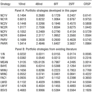
Table 5 Portfolio Turnovers

NC1V 01494 02680 01729 02407 06141 NC1R 06013 08232 10064 09767 09753 NC2V 01448 03266 01946 04570 05808 NC2R 10177 27556 16594 36275 10443 NCFV 01052 02469 02790 04134 05729 NCFR 06944 23117 19952 33560 10584 PARV 01689 03838 02600 04628 05743 PARR 10414 24846 16407 35657 10984

Panel B: Portfolio strategies from existing literature

1/N 00232 00311 00155 00174 00595 VW 00382 00540 00213 00310 02316 MEAN 10135 1056126 07987 42495 30014 BAYE 03565 66314 05388 21264 06191 MINU 01656 08286 02223 07953 07769 MINC 00552 00741 00461 00841 04222 FAC1 00935 02047 01152 02398 03650 LWID 01132 04029 00905 03144 05594 LW1F 01428 04034 01455 04893 05463 BSV3 04683 09066 05384 05564 21926

Notes. This table reports the monthly turnover of the various portfolios. Turnover is the average percentage of wealth traded in each period and, as deﬁned in Equation (13), is equal to the sum of the absolute value of the rebalancing trades across theNavailable assets and over theT₋₋1 trad-ing dates, normalized by the total number of tradtrad-ing dates.

However, the F-norm-constrained portfolio

cali-brated by maximizing the return of the portfolio in the previous period (NCFR) fails to achieve higher Sharpe ratios than the corresponding LW1F portfolio. Finally, even though the PARR portfolio does not use firm-specific characteristics, it achieves Sharpe ratios that are at least as good as those for the para-metric portfolios (BSV) developed in Brandt et al. (2005), and the differences are significant for the 10Ind and CRSP data sets.

From panel A of Table 5 we see that the turnover of the norm-constrained portfolios calibrated using cross validation over the portfolio variance is much lower than that of the portfolios calibrated by maximiz-ing the portfolio return. Panel B of this table shows, not surprisingly, that the best portfolios in terms of

turnover are the 1/N and value-weighted portfolios.17

The turnover of these portfolios is followed by that of the shortsale-constrained minimum-variance portfolio

(MINC). The turnovers of the 1-, 2-, and F

-norm-constrained portfolios and the partial minimum-variance portfolio calibrated with cross validation

17_{We compute the value-weighted portfolio for each data set as the}

portfolio that assigns a weight to each asset equal to the market capitalization of that asset divided by the market capitalization of all the assets in the data set. Note that because the composition of the “market portfolio” may be changing over time, the strategy of holding the value-weighted portfolio may have a turnover that is different from zero.

over variance, and the LWID and LW1F portfolios proposed in Ledoit and Wolf (2003, 2004), are higher than that of MINC. The shortsale-unconstrained minimum-variance portfolio and the portfolios based on factor models have higher turnover than MINC and the norm-constrained strategies calibrated to minimize portfolio variance. The partial minimum-variance portfolio calibrated by maximizing the port-folio return in the last month (PARR) and the para-metric portfolios based on the work by Brandt et al. (2005) have similar turnovers, which are much higher than those of the rest of the portfolios.

5. Conclusion

We provide a general unifying framework for deter-mining portfolios in the presence of estimation error. This framework is based on shrinking directly the portfolio-weight vector rather than some or all of the elements of the sample covariance matrix. This is accomplished by solving the traditional minimum-variance problem (based on the sample cominimum-variance matrix) but subject to the additional constraint that the norm of the portfolio-weight vector be smaller than a given threshold. We show that our gen-eral framework nests as special cases the shrinkage approaches of Jagannathan and Ma (2003), Ledoit

and Wolf (2003, 2004), and the 1/N portfolio

stud-ied in DeMiguel et al. (2007). We also compare empirically the out-of-sample performance of the new portfolios we have proposed to 10 strategies in the literature across ﬁve data sets. We ﬁnd that the norm-constrained portfolios often have a higher Sharpe ratio than the portfolio strategies in Jagannathan and

Ma (2003), Ledoit and Wolf (2003, 2004), the 1/N

port-folio, and other strategies in the literature, such as factor portfolios.

6. Electronic Companion

An electronic companion to this paper is available as part of the online version that can be found at http:// mansci.journal.informs.org/.

Acknowledgments

The authors gratefully acknowledge ﬁnancial support from INQUIRE-UK; however, this article represents the views of the authors and not of INQUIRE. The third author is par-tially supported by the Ministry of Education and Science and Technology of Spain through CICYT Project MTM2007-63140. The authors are very grateful to Department Edi-tor David Hsieh, the associate ediEdi-tor, and two anonymous referees for detailed and extensive comments. The authors thank Mike Chernov, Wayne Ferson, Vito Gala, Michael Gallmeyer, Francisco Gomes, Burton Holliﬁeld, Garud Iyen-gar, Tongshu Ma, Igor Makarov, Spencer Martin, Javier Peña, Roberto Rigobon, Pedro Santa Clara, Chester Spatt, Catalina Stefanescu, and Bruce Weber for comments. The